Nodal line estimates for the second Dirichlet eigenfunction
Thomas Beck, Yaiza Canzani, Jeremy L. Marzuola

TL;DR
This paper analyzes the structure and curvature of nodal lines of low-energy Dirichlet eigenfunctions in curvilinear quadrilaterals, extending previous methods and providing precise bounds with applications to spectral theory.
Contribution
It generalizes existing tools to study nodal curves in more complex domains, offering detailed curvature bounds and insights for small aspect ratios.
Findings
Derived uniform curvature bounds for nodal curves
Extended analysis to domains with small aspect ratios
Discussed implications for Courant-sharp eigenfunctions
Abstract
We study the nodal curves of low energy Dirichlet eigenfunctions in generalized curvilinear quadrilaterals. The techniques can be seen as a generalization of the tools developed by Grieser-Jerison in a series of works on convex planar domains and rectangles with one curved edge and a large aspect ratio. Here, we study the structure of the nodal curve in greater detail, in that we find precise bounds on its curvature, with uniform estimates up to the two points where it meets the domain at right angles, and show that many of our results hold for relatively small aspect ratios of the side lengths. We also discuss applications of our results to Courant-sharp eigenfunctions and spectral partitioning.
Click any figure to enlarge with its caption.
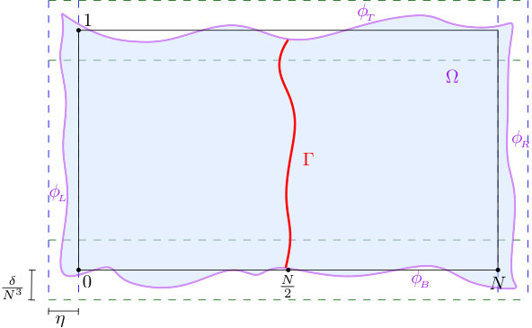 Figure 1
Peer Reviews
No public reviews on file for this paper yet. If you reviewed it on a platform where reviews are public (OpenReview, ICLR, NeurIPS, ICML), you can paste yours below so the community can read it here.
Videos
No videos yet. Explain this paper in a talk, walkthrough, or lecture? Add one.
Nodal line estimates for the second Dirichlet eigenfunction
Thomas Beck
Department of Mathematics, University of North Carolina at Chapel Hill
CB#3250 Phillips Hall
Chapel Hill, NC 27599
,
Yaiza Canzani
Department of Mathematics, University of North Carolina at Chapel Hill
CB#3250 Phillips Hall
Chapel Hill, NC 27599
and
Jeremy L. Marzuola
Department of Mathematics, University of North Carolina at Chapel Hill
CB#3250 Phillips Hall
Chapel Hill, NC 27599
Abstract.
We study the nodal curves of low energy Dirichlet eigenfunctions in generalized curvilinear quadrilaterals. The techniques can be seen as a generalization of the tools developed by Grieser-Jerison in a series of works on convex planar domains and rectangles with one curved edge and a large aspect ratio. Here, we study the structure of the nodal curve in greater detail, in that we find precise bounds on its curvature, with uniform estimates up to the two points where it meets the domain at right angles, and show that many of our results hold for relatively small aspect ratios of the side lengths. We also discuss applications of our results to Courant-sharp eigenfunctions and spectral partitioning.
1. Introduction and statement of results
Understanding the fundamental modes of vibration of a compact domain is a longstanding problem. The original motivation was to describe how a metal sheet with a given shape would vibrate when struck at some fundamental frequency. The main goal being to understand the structure of the set of points in the sheet that are stable, i.e. that are not vibrating. These non-vibrating regions are the zero sets of the Laplace eigenfunctions corresponding to solving the Helmholtz equation on the domain that represents the metal sheet. In the 17th century R. Hook observed these patterns by spilling sand on a glass sheet, and striking the sheet with a violin bow. When the sheet starts vibrating, the sand rearranges itself across the sheet until it is placed on the non-vibrating areas, thus exhibiting the zero sets for the corresponding eigenfunction. This experiment was later reproduced by E. Chladni, who was the first to record an extensive list of zero set configurations. It is nowadays known as the Chladni plates experiment.
We dedicate this article to giving a precise description of the structure of the zero set of the second eigenfunction for a planar domain whose shape is obtained after perturbing a rectangle. While we focus on the second Dirichlet eigenfunction, the techniques developed here can be applied to the low-lying eigenfunctions in general up to a frequency depending upon the length of the domain. Also, there are natural generalizations to Neumann (or more generally Robin) boundary conditions, but for the sake of clarity and presentation we will focus on Dirichlet domains at present.
We note that low-lying eigenvalues and eigenfunctions of the Laplacian on a compact domain also play a role in understanding random walks ([KP89]), heat conductivity ([S*+*96]) and more. See for instance the recent works [Zel17, Ste17] and references therein for a nice overview of applications and modern topics in the theory of eigenfunctions and nodal sets.
In this work, we study the second Dirichlet eigenfunction of the Laplacian on a planar domain , so that
[TABLE]
where is the corresponding eigenvalue. The domain is a curvilinear rectangle that is very nearly rectangular in a Gromov-Hausdorff sense to be made precise below in (2). For convenience, we normalize so that . We are interested in studying the nodal set of , which we denote by
[TABLE]
To do this we build off the pioneering works of Jerison [Jer95] and Grieser-Jerison [GJ96, GJ98, GJ09], who studied the low energy eigenfunctions in convex domains and rectangles of high aspect ratio with one curved edge. For convex domains they studied the location of the maximum and nodal line of the first and second Dirichlet eigenfunction respectively, giving estimates that are uniform as the eccentricity of the domain increases. They also derived a method to do a very detailed asymptotic analysis of the location of the nodal line or the location of the maximum for low energy Dirichlet eigenfunction in a rectangle with one curved side. This method is the starting point for our work on curvilinear rectangles.
On a rectangle, the zero set of the second eigenfunction for the Laplacian is a straight line, perpendicular to the long sides, that divides the rectangle in two equal pieces. Here, we study the zero set of the second eigenfunction on a region that is a perturbation of a rectangle. Indeed, we extend the results in [GJ09] to explore the precise dependence of the nodal set on the properties of the bounding curves and the aspect ratio of the underlying region .
We obtain estimates on the width and regularity of the nodal line of , with explicit bounds, tracking how the slope and curvature of the nodal line depend upon the top and bottom curve. In particular, we show that there are distinct differences in the nodal line depending upon if some of the bounding curves are flat or if they are curved. As we are imposing Dirichlet boundary conditions, the eigenfunction vanishes on the boundary of the domain, and analyzing the behavior of the nodal line becomes increasingly delicate as it approaches the boundary. Our techniques allow us to obtain estimates that are uniform up to the boundary and show that the nodal line meets the boundary of orthogonally at two points.
To state our results precisely, we first define the class of domains under consideration. Let be functions defining a region in that is a perturbation of the rectangle , for , of the form
[TABLE]
The functions , defining the sides of the domain are in , with
[TABLE]
for and some . The functions , defining the top and bottom are in , with
[TABLE]
for and constants . Here , and . Note that as , tend to [math], the domain becomes rectangular.
In the case of the rectangle with , the second Dirichlet eigenfunction is given by and the nodal line is precisely the straight line . The theorem below shows how changes under the above perturbations of the rectangle. Let be the projection onto the -axis.
Theorem 1.1**.**
There exist , , such that and has diameter bounded by
[TABLE]
Moreover, there exists a function such that , with
[TABLE]
The nodal line touches the boundary of at precisely points, and it meets the boundary orthogonally at these points.
Here and throughout, constants denoted by , , etc depend on the constants , but are independent of , , and . (In fact we will only require control on derivatives up to .)
An immediate feature to note is that in the special case of flat upper and lower boundaries (, ), we can set and the factor of does not appear in the estimates of Theorem 1.1. Therefore, in this flat case the diameter of the nodal line, , is exponentially small in (rather than the polynomial decay in when ).
From Theorem 1.1 we see that for sufficiently large (and ), the perturbation of the nodal line from straight is smaller than that of the side perturbations , . In the flat case, , , we can track the constants in the proof of Theorem 1.1 (see Section 5) to obtain an explicit lower bound on the size of required for this to occur:
Corollary 1.1**.**
There exists a constant such that for and ,
[TABLE]
In the flat case, , , for each , we can take sufficiently small so that the above estimates hold.
By controlling the behavior of the nodal line up to the boundary, we are able to show for the class of domains under consideration that the nodal line is not closed, but meets the boundary (orthogonally) at two points. More generally, Payne [Pay67] conjectured that the nodal line of the second eigenfunction of a bounded planar domain touches the boundary at points. This was proved for smooth, convex domains by Melas [Mel92], but a counterexample (for a non-simply connected planar domain) was given by Hoffmann-Ostenhof, Hoffmann-Ostenhof, and Nadirashvili [HOHON97].
In [FK08], Freitas and Krejc̆ir̆ík study the Dirichlet Laplacian for a class of thin curved tubes. As the volume of the cross-section tends to [math] they establish the convergence of the eigenvalues and eigenfunctions in terms of an ordinary differential operator on the base curve of the tube. In particular, they locate the nodal set to sufficient precision to also deduce that the nodal set must intersect the boundary. Krejc̆ir̆ík and Tus̆ek also prove an analogous result for domains consisting of a thin tubular neighborhood of a hypersurface, [KT15]. The idea of reducing to an associated ordinary differential operator has also been used extensively by Friedlander-Solomyak [FS08], [FS09] and Borisov-Freitas [BF09] to obtain asymptotics of the eigenvalues, eigenfunctions, and resolvent of the Dirichlet Laplacian in thin domains.
Applications to partitioning algorithms
Recently, in work on graph and data partitioning algorithms, Szlam et al in [SMCB05, Szl09] observed that if one partitions very general geometric graphs using cuts along nodal lines of the graph Laplacian, that the regions tend towards rectangles of bounded aspect ratios. The underlying idea of graph partitions are for instance to cluster data points or to provide a good foundation for a wavelet basis to name just two. There is also the continuum limit version of this, in which one could ask to partition a planar domain using the first non-trivial Neumann or second Dirichlet eigenfunction respectively. Again, for a very general boundary, one expects that such partitions would converge rapidly to a set of near rectangles.
We can use Corollary 1.1 to demonstrate such a convergence: In the flat case, with , and sufficiently small, we perform the following iteration procedure. Given such a domain , with flat top and bottom boundaries, we form new domains by cutting along the nodal line . By then rescaling each domain in the -direction, and using the estimates above, we can ensure that these two new domains are of the form of , for appropriate chosen functions and , and satisfy the bounds
[TABLE]
In other words, these new sides to the domain satisfy the original bounds in (3), but with replaced by . Iterating this process of cutting along the nodal line, will therefore give domains converging (in a Hausdorff sense) to an exact rectangle. Analogously, for the general top and bottom boundaries considered here, using the estimates in Corollary 1.1, given , , with , and for sufficiently large, we can repeat the above iteration process, to again give a sequence of domains converging to a rectangle.
Another partitioning related to the nodal set of Dirichlet eigenfunctions of the Laplacian is the following: Given a domain and integer , a spectral minimal k-partition of is a partition of into disjoint sets that minimizes . Here is the first Dirichlet eigenvalue of . If , then the spectral minimal partition is given by the nodal domains of a second Dirichlet eigenfunction of . More generally, if a -th Dirichlet eigenfunction has exactly -nodal domains (and so gives equality in the Courant nodal domain Theorem), then these nodal domains form a minimal -partition. See the survey paper of Helffer [Hel10] for greater discussion of spectral minimal partitions and references. It is therefore important to classify examples where the Courant nodal domain Theorem is sharp, and in [HHOT09] they show that the third Dirichlet eigenfunction of the rectangle has three nodal domains whenever the aspect ratio is greater than . Using the techniques presented here, for any fixed , by taking sufficiently large, for all , the -th Dirichlet eigenfunction has exactly nodal domains (with nodal set approximately equal to the union of the lines for ). Thus, in this case, the nodal domains will provide a spectral minimal -partition.
Outline of the paper
The structure of the rest of the paper as follows: In Section 2 we describe an adiabatic approximation of the eigenfunction that is a key ingredient in the proof of Theorem 1.1. This type of approximation, which can be viewed as an approximate separation of variables for our approximately rectangular domain, has been used in the work of Grieser and Jerison [GJ96], [GJ09]. The approximation has also been used in [BSS97] for numerical analysis of eigenfunctions in partially rectangular billiards, and in [HM12] to analyze non-concentration of eigenfunctions in partially rectangular billiards. In Section 3, we establish the desired properties of the width and regularity of the nodal line using the adiabatic approximation. Then, in Section 4 we demonstrate how in the flat case, we have simple ODE estimates to establish the approximation, and following this, we prove the error estimates for the approximation for our general class of domains. Lastly, in Section 5 we compute an explicit Hadamard variation formula to evaluate the effect the side perturbations have on the eigenfunction. This will in particular allow us to track the constants appearing in the proof of Theorem 1.1 in the flat case and prove Corollary 1.1.
Acknowledgements
This project was started due to a conversation with Stefan Steinerberger and Hau-tieng Wu, who pointed us to the work of [Szl09] as motivation to understand nodal line partitioning in domains, and with whom the third author is exploring a related question for the -Laplacian on curvilinear rectangles. YC is supported in part by the Sloan Foundation. JLM acknowledges support from the NSF through NSF CAREER Grant DMS-1352353.
2. The Adiabatic Ansatz
A key ingredient in the proof of Theorem 1.1 is to establish properties of a Fourier decomposition of the eigenfunction . For convenience, we introduce the height function
[TABLE]
and note that (4) we have for all . For with , we write as
[TABLE]
where
[TABLE]
We will view the first term in the right hand side of (5) as the main term, with an error term when is large, and , are small. The function is the first Fourier mode in the -direction, given by
[TABLE]
To prove Theorem 1.1 we will use this decomposition of , and will require a lower bound on , together with upper bounds on , and their derivatives. In fact, to prove the estimates on regularity of the nodal line near , we need to consider a larger class of decompositions of : Given , suppose that , with and . Next, let the linear isometry built by rotating about the point and then translating in such a way that if , then . In general, write for the new system of coordinates. We then define to be equal to the eigenfunction in these rotated coordinates,
[TABLE]
Remark 2.1**.**
By the bounds on and from (4), there exists such that the angle of rotation is bounded by .
The function satisfies
[TABLE]
in the domain
[TABLE]
with . In particular, for , we have . Here , satisfy the bounds
[TABLE]
[TABLE]
. Up to the factor of , the derivative bounds are the same as for , . Moreover, by the construction of , we have . The functions , satisfy
[TABLE]
[TABLE]
for . We can make the analogous definition if the closest point to lies on the upper boundary of . For ease of notation, we now drop the tildes, and for each function coming from such a rotation, for we write
[TABLE]
where
[TABLE]
for the new height function . To prove Theorem 1.1, we will use the proposition below which gives properties of these decompositions.
Proposition 2.1**.**
There exist positive constants , such that the following properties hold: For each decomposition, there exists a unique point such that , and this point lies in the interval . Moreover, for ,
[TABLE]
and for , , we have
[TABLE]
Proposition 2.1 is proved in Section 4.
Remark 2.2**.**
When the rotation is trivial, is equal to and the decomposition reduces to the one for given in (5). Therefore, the properties in this proposition also hold for and . In fact, in this case, the unique point where lies in the interval
[TABLE]
3. Estimates on the nodal line
In this section we will prove Theorem 1.1 assuming that Proposition 2.1 holds. We first establish an upper bound on the width of the projection to the -axis of the nodal line in terms of the error and its derivatives. We will require a different argument to control the behavior of the nodal line near the boundary, and so we set
[TABLE]
We continue to write and . Since for all , we have that on and on . Therefore, this choice yields
[TABLE]
and similarly
[TABLE]
Using the decomposition of from (5), define to be the smallest interval with and such that
- A)
2. B)
Lemma 3.1**.**
If , then for all .
- Proof of Lemma 3.1: Let . Then, and so
[TABLE]
By assumption (A), this is strictly positive. Now let . Then, since , we have . Also, using that we obtain
[TABLE]
and by assumption (B) this is strictly positive. The case is treated in the same way.
Using Proposition 2.1, we let be the unique point in the interval where . Define the interval ,
[TABLE]
where
[TABLE]
Lemma 3.2**.**
If , then for all .
[TABLE]
Also, since , we have . Therefore, provided
[TABLE]
and the latter always holds if .
Now let . Then, as in (10)
[TABLE]
and using gives
[TABLE]
Therefore, from the definition of , for .
Using Proposition 2.1 and Remark 2.2, there exist and such that and , and so the estimate on the width and location of the nodal line in Theorem 1.1 follows immediately from Lemma 3.2.
To study the regularity of the nodal line, we use the coordinate change described in Section 2. For a given with , , this coordinate change transforms to and the eigenfunction to . Dropping the tildes, we have in the domain
[TABLE]
with . Moreover, . Setting , , we decompose as in (8). Note that in the case of a flat top and bottom boundary, the coordinate change is trivial, and is identically equal to . The case is treated in the analogous way by making a rotation about the top boundary.
We set , and to establish the regularity of the nodal line, we first study it away from the boundary of . Define
[TABLE]
and
[TABLE]
We will show in the proof of Lemma 3.3 that provides a lower bound for for points with .
Lemma 3.3**.**
Suppose that . Then, for every with there exist a smooth real valued function and a neighborhood of such that
[TABLE]
with
[TABLE]
- Proof of Lemma 3.3: Note that for all
[TABLE]
and
[TABLE]
Therefore,
[TABLE]
Let , and suppose that . Then, using
[TABLE]
with as defined in (12). Thus, since by assumption. This implies the existence of the graph function along a neighborhood of . Note that for every
[TABLE]
We next find an upper bound for . Since for all
[TABLE]
then
[TABLE]
This together with (15) yield the claimed bound on when .
To study the regularity of the nodal line near , we define
[TABLE]
and
[TABLE]
We will show in Lemma 3.4 that provides a lower bound for for all points .
Lemma 3.4**.**
If , there exist a neighborhood of , and smooth real valued function , such that and
[TABLE]
Furthermore, meets orthogonally.
- Proof of Lemma 3.4: Since , we have , and so
[TABLE]
In addition, using , we know that and . Therefore,
[TABLE]
This proves the existence of . For , with we have . Therefore,
[TABLE]
Note that with for . Since , it follows that
[TABLE]
Moreover,
[TABLE]
for some , and
[TABLE]
for some . In particular, ( ‣ 3) yields
[TABLE]
Next, note that since , there exists such that . Since for , it follows that
[TABLE]
Therefore,
[TABLE]
In the same way, we have
[TABLE]
and
[TABLE]
To improve (23) and obtain a in the upper bound, we need better control on in (22). To do this we note
[TABLE]
where the last equality was obtained after differentiating twice and using . From (23) it follows that for and ,
[TABLE]
The bound on follows from combining (16) with (20) and (26). In particular , showing that meets orthogonally.
Applying Proposition 2.1, the estimate on given in Theorem 1.1 follows immediately from Lemmas 3.3 and 3.4. The following lemma gives the desired uniform bound on and completes the proof of Theorem 1.1:
Lemma 3.5**.**
There exist constants , such that
[TABLE]
- Proof of Lemma 3.5: Let be a point on the nodal line . Then, differentiating twice gives the expression
[TABLE]
To bound the denominator, we use the lower bounds on from (15) (in the centre) and (20) (near the boundary). By Proposition 2.1 this implies that
[TABLE]
We also have upper bounds on from (17) (in the centre) and (26) (near the boundary), which again using Proposition 2.1 gives
[TABLE]
Finally, from Proposition 2.1 we have , , and combining (25) with
[TABLE]
gives
[TABLE]
Using these estimates gives the desired bound for the expression for in (27).
Remark 3.1**.**
In the case of flat upper and lower boundaries, we have the following estimates on the quantities appearing in the numerator of (27): First, satisfies
[TABLE]
where in the second inequality we have used (23) (and the fact that in the flat case). We also immediately have the estimates on the second derivatives of of
[TABLE]
Finally,
[TABLE]
where in the second inequality, we have used , and that in the flat case. We will use these estimates in Section 5 when we explicitly track the constants in the flat case.
4. Proof of Proposition 2.1
In this section we will prove Proposition 2.1 by establishing the required properties of the decompositions of and defined in (5) and (8). From the definition of the domain from (2), contains the rectangle , and is contained in the rectangle . Therefore, by domain monotonicity for Dirichlet eigenvalues we have the following lemma.
Lemma 4.1**.**
The second Dirichlet eigenvalue satisfies
[TABLE]
The boundary of is smooth, except at four points where the -curves meet at a convex angle. This ensures that the gradient of is bounded.
Lemma 4.2**.**
There exists a constant depending only on , from (4) such that for . In particular, from (3), for all , we have
[TABLE]
We recall that the function satisfies in the domain as in (11), with . We recall that , , , , satisfy the bounds (6) and (7). Since is equal to in the rotated coordinates, by Lemma 4.2 we have
[TABLE]
Defining a height function by , we write as the Fourier series
[TABLE]
Here the -th mode is given by
[TABLE]
To prove Proposition 2.1, we will first bound each mode , then sum over , and finally use elliptic estimates to extend these to derivative bounds. To estimate , we use the eigenfunction equation to find the equation that it satisfies, and then use the Duhamel principle to find an implicit expression. To bound this expression we need control on the boundary values , .
Lemma 4.3**.**
There exists a constant such that
[TABLE]
- Proof of Lemma 4.3: By definition
[TABLE]
As noted in Remark 2.1, the angle of rotation in the definition of is bounded by for some . Since vanishes on , Lemma 4.2 implies that
[TABLE]
Inserting this into (29) gives the estimate for . The estimate for follows in the same way.
Proof of Proposition 2.1: Flat case
Let us first consider the case of a flat top and bottom, with , and , . In this case, we can remove the factor of in the estimate in Lemma 4.3 above. Using that for , the function satisfies the ODE
[TABLE]
Writing for (by Lemma 4.1, provided ), we therefore have, for ,
[TABLE]
Writing as in (5), this expression gives , and likewise for derivatives of . For ,
[TABLE]
and we set . The function satisfies
[TABLE]
Setting gives , and since , this implies that . The estimates from Proposition 2.1 then follow readily from the expressions in (31) and (32).
Proof of Proposition 2.1: General case
In the general case, satisfies an approximate version of the ODE in (30), with an error depending on , and their first two derivatives: Fix , and set
[TABLE]
Lemma 4.4**.**
The function satisfies the equation
[TABLE]
where has the bound
[TABLE]
for an absolute constant .
- Proof of Lemma 4.4: The function is equal to
[TABLE]
Applying the bounds we have derived for in (28) and the definition of in (33), the terms that do not immediately obey the estimate of the lemma are the first term and the term in the final integral given by
[TABLE]
This is because this is the only term in the final integral in (34) for which a factor appears in the expression for . All of the other terms in the last two integrals in (34) contain at most one derivative of , two derivatives of and , and one factor of . After an integration by parts is equal to
[TABLE]
and (35) can be written as
[TABLE]
Since is bounded by a constant, both of these terms are of the desired form.
The function also satisfies the boundary conditions
[TABLE]
where are values coming from the side variation of the domain, wih bounds in Lemma 4.3.
For , set and for , set .
Lemma 4.5**.**
Define the functions and (for ) by
[TABLE]
Then,
[TABLE]
with . Also,
[TABLE]
for constants , , with
[TABLE]
- Proof of Lemma 4.5: The functions and satisfy
[TABLE]
The lemma then follows from Lemma 4.4 and the boundary conditions of at .
Combining Lemmas 4.4 and 4.5, we can bound .
Proposition 4.1**.**
There exist constants , , such that for , ,
[TABLE]
Here is the distance of from the endpoints of .
- Proof of Proposition 4.1: We fix , and use Lemmas 4.4 and 4.5 to bound at (with a bound independent of ). The constants , from Lemma 4.5 can be written for as
[TABLE]
with . From Lemma 4.4, we have the bound
[TABLE]
and from Lemma 4.3, . Therefore, since , the only terms in the expression for from Lemma 4.5 that do not immediately satisfy the required estimates are
[TABLE]
However, these integrals can be combined to be written as
[TABLE]
Using the bound on from (36) and integrating gives the desired bound.
We write
[TABLE]
Summing the estimate from Proposition 4.1 over we can control the -norm of . For the rest of the section, fix and denote the cross-section at by .
Corollary 4.1**.**
There exist constants , such that
[TABLE]
We now convert this -estimate into bounds on derivatives of .
Proposition 4.2**.**
For each , and with as in Corollary 4.1, there exists a constant such that
[TABLE]
- Proof of Proposition 4.2: To obtain this estimate on we find the elliptic equation that it satisfies. For , we have
[TABLE]
The function consists of terms where at least one derivative in has been applied to a factor of or , and so for each , there exists a constant such that
[TABLE]
Using the eigenfunction equation, satisfies
[TABLE]
Applying elliptic estimates to this equation, (38) and the estimate on from Corollary 4.1 establishes the proposition.
Using Proposition 4.2, we can obtain more refined information about the first Fourier mode and complete the proof of Proposition 2.1.
Proposition 4.3**.**
There exists a constant such that in the interval the function has a unique zero at with . Moreover, for this range of , and for , , we have,
[TABLE]
Here the constant is as in Lemma 4.5 and satisfies .
- Proof of Proposition 4.3: By Lemma 4.1, for a constant . Therefore, using the expression for from Lemma 4.5 and the bound from Lemma 4.4, we have
[TABLE]
Here is a constant (changing from line-to-line). Moreover, since , and
[TABLE]
combining (40) with Proposition 4.2, we have
[TABLE]
To complete the proof of the lemma, we need to bound . Differentiating the expression from Lemma 4.5 gives
[TABLE]
In particular , and combining this with the estimate for gives the required bound for . The expression for from Lemma 4.4 gives , and differentiating we have . Since is non-zero on , has at most one zero in this interval. The function has its unique zero in this interval at , with , and its derivative is bounded below by . Therefore, also has a unique zero at , with .
Remark 4.1**.**
In the case that no rotation has been applied (so that ), the function from Lemma 4.4 satisfies the stronger bound . Inserting this stronger estimate into the argument above, the point satisfies .
5. An explicit Hadamard variation formula and constant tracking
To prove Proposition 2.1, we used the estimate on the boundary values of the Fourier modes, and , in Lemma 4.3, which follows only from a gradient estimate on the eigenfunction. In order to track the constants appearing in the error estimates in Proposition 2.1 in the flat case, we require a more explicit bound on these boundary values. We do this as follows, using a variant of a calculation given in [GJ09].
Proposition 5.1**.**
There exists a constant such that
[TABLE]
- Proof of Proposition 5.1: We extract the main term in as follows. First, we integrate by parts to write as
[TABLE]
The domain is the domain . The second integral in (42) is bounded in absolute value by . The first integral in (42) consists of three terms. Two of these integrals are over portions of the top and bottom boundaries of of length bounded by , and so since the gradient of is bounded, these integrals are bounded in absolute value by . The remaining contribution to (42) is given by
[TABLE]
To pick out the main term in (43) we write
[TABLE]
with and for an error term to be estimated below. Using , (43) becomes
[TABLE]
up to an error . We are left to bound the second integral in (44), and to do this we will use the results of Section 4 to estimate . Summing the estimate from Proposition 4.1 over , we obtain a bound on for of
[TABLE]
for constants , , where we recall that is the cross-section of at . Combining this with Proposition 4.3 shows that for , we have
[TABLE]
Using Lemma 4.2, we can also bound in a different way for via
[TABLE]
In particular, using (45) and (46), we have . Moreover, satisfies the equation
[TABLE]
We can use this to bound the second integral in (44). Let be a smooth cut-off function, equal to for and [math] for . There exists an extension of \sin(\mu_{1}(N-x))\sin(\tilde{\beta}(0,y))\big{|}_{x=\rho_{L}(y)} to , with such that
[TABLE]
The function therefore vanishes on , and satisfies
[TABLE]
Elliptic estimates therefore imply that
[TABLE]
Using , we have the same bound on . Elliptic estimates thus give , where . Applying this estimate in the second integral in (44), we see that the integral can be bounded by , and this therefore concludes the proof of the proposition.
Now consider the case where the domain has flat top and bottom boundaries (so that , ). Proposition 5.1 then allows us to track the constants appearing in the error estimates in Proposition 2.1: Given (not necessarily large) and a small constant , we can choose sufficiently small so that
[TABLE]
By choosing small compared to , we can use this in (31) and (32) to get explicit estimates on and its derivatives, with the estimates not depending on any unknown constants. Using this in the quantities appearing in Section 3, for any fixed and sufficiently small, this provides the following bounds and proves Corollary 1.1: We have
[TABLE]
where we recall from Lemma 3.2 that the width of the nodal line is bounded by . Moreover, we have
[TABLE]
and from Lemmas 3.3 and 3.4 this gives the upper bound on of
[TABLE]
Finally, inserting the bounds from Remark 3.1 on the terms appearing in gives
[TABLE]
The reference list from the paper itself. Each links out to its DOI / PubMed record.
- 1[BF 09] Denis Borisov and Pedro Freitas. Singular asymptotic expansions for Dirichlet eigenvalues and eigenfunctions on thin planar domains. Ann. Inst. H. Poincaré Anal. Non Linéaire , 26:547–560, 2009.
- 2[BSS 97] Arnd Bäcker, Roman Schubert, and Peter Stifter. On the number of bouncing ball modes in billiards. Journal of Physics A: Mathematical and General , 30(19):6783, 1997.
- 3[FK 08] Pedro Freitas and David Krejc̆ir̆ík. Location of the nodal set for thin curved tubes. Indiana Univ. Math. J. , 57(1):343–375, 2008.
- 4[FS 08] Leonid Friedlander and Michael Solomyak. On the spectrum of narrow periodic waveguides. Russian J. of Math. Physics , 57(1):238–242, 2008.
- 5[FS 09] Leonid Friedlander and Michael Solomyak. On the spectrum of the Dirichlet Laplacian in a narrow strip. Israel J. Math. , 170:337–354, 2009.
- 6[GJ 96] Daniel Grieser and David Jerison. Asymptotics of the first nodal line of a convex domain. Inventiones mathematicae , 125(2):197–219, 1996.
- 7[GJ 98] Daniel Grieser and David Jerison. The size of the first eigenfunction of a convex planar domain. J. Amer. Math. Soc. , 11(1):41–72, 1998.
- 8[GJ 09] Daniel Grieser and David Jerison. Asymptotics of eigenfunctions on plane domains. Pacific journal of mathematics , 240(1):109–133, 2009.