Symmetry-Enriched Quantum Spin Liquids in $(3+1)d$
Po-Shen Hsin, Alex Turzillo

TL;DR
This paper classifies symmetry-enriched quantum spin liquids in (3+1)d using higher-form symmetries, providing a systematic framework for understanding their phases, anomalies, and dualities.
Contribution
It introduces a classification scheme for (3+1)d symmetry-enriched phases based on higher-form symmetries and their couplings, extending previous (2+1)d results.
Findings
Classified (3+1)d symmetry-enriched phases using higher-form symmetries.
Identified a systematic method for constructing symmetry protected topological phases.
Discovered a tension with a conjectured duality in (3+1)d $SU(2)$ gauge theory.
Abstract
We use the intrinsic one-form and two-form global symmetries of (3+1) bosonic field theories to classify quantum phases enriched by ordinary (-form) global symmetry. Different symmetry-enriched phases correspond to different ways of coupling the theory to the background gauge field of the ordinary symmetry. The input of the classification is the higher-form symmetries and a permutation action of the -form symmetry on the lines and surfaces of the theory. From these data we classify the couplings to the background gauge field by the 0-form symmetry defects constructed from the higher-form symmetry defects. For trivial two-form symmetry the classification coincides with the classification for symmetry fractionalizations in . We also provide a systematic method to obtain the symmetry protected topological phases that can be absorbed by the coupling, and we give the…
Click any figure to enlarge with its caption.
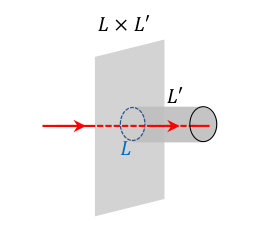 Figure 1
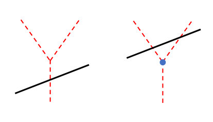 Figure 2
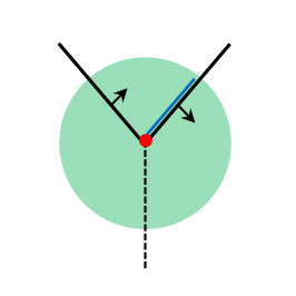 Figure 3
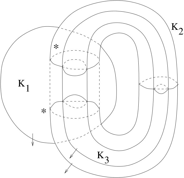 Figure 4
| Electric | Magnetic | Backgrounds |
|---|---|---|
| boson, | boson | |
| boson, | boson | , |
| fermion, | boson | , |
| fermion, | boson | , |
| boson, | fermion | , |
| boson, | fermion | , |
| Electric | Magnetic | Backgrounds |
|---|---|---|
| fermion, | fermion | , |
| non-trivial generators of SPT phases | ||
|---|---|---|
| 0 | ||
| 0 | ||
| 0 | ||
| 0 |
| Electric | Magnetic | Backgrounds |
|---|---|---|
| boson, , tensor | boson, tensor | |
| boson, , spinor | boson, tensor | |
| boson, , tensor | boson, spinor | |
| boson, , tensor | boson, tensor | , |
| boson, , spinor | boson, tensor | , |
| fermion, , tensor | boson, tensor | , |
| fermion, , spinor | boson, tensor | , |
| fermion, , tensor | boson, tensor | , |
| fermion, , spinor | boson, tensor | , |
| boson, , tensor | fermion, tensor | , |
| boson, , tensor | fermion, spinor | , |
| boson, , tensor | fermion, tensor | , |
| fermion, , spinor | boson, spinor | , |
| boson, , spinor | fermion, spinor | , |
Peer Reviews
No public reviews on file for this paper yet. If you reviewed it on a platform where reviews are public (OpenReview, ICLR, NeurIPS, ICML), you can paste yours below so the community can read it here.
Videos
No videos yet. Explain this paper in a talk, walkthrough, or lecture? Add one.
\savesymbol
iint \savesymboliiint \restoresymbolTXFiint \restoresymbolTXFiiint
Symmetry-Enriched Quantum Spin Liquids in
Abstract
We use the intrinsic one-form and two-form global symmetries of (3+1) bosonic field theories to classify quantum phases enriched by ordinary ([math]-form) global symmetry. Different symmetry-enriched phases correspond to different ways of coupling the theory to the background gauge field of the ordinary symmetry. The input of the classification is the higher-form symmetries and a permutation action of the [math]-form symmetry on the lines and surfaces of the theory. From these data we classify the couplings to the background gauge field by the 0-form symmetry defects constructed from the higher-form symmetry defects. For trivial two-form symmetry the classification coincides with the classification for symmetry fractionalizations in . We also provide a systematic method to obtain the symmetry protected topological phases that can be absorbed by the coupling, and we give the relative ’t Hooft anomaly for different couplings. We discuss several examples including the gapless pure gauge theory and the gapped Abelian finite group gauge theory. As an application, we discover a tension with a conjectured duality in for gauge theory with two adjoint Weyl fermions.
Contents
-
1.2 One-form symmetry that acts trivially on all lines in TQFT
-
2 Classification of symmetry-enriched phases from higher-form symmetry
-
2.2 Symmetry defects from higher-codimension symmetry defects
1 Introduction
In this note we investigate the problem of classifying different ways of coupling a conformal field theory (in the broad sense including topological quantum field theory) in to the background gauge field of an ordinary global symmetry. Such theories are said to be enriched by the global symmetry. They can arise as the low energy effective descriptions of microscopic lattice models. Since such theories are fixed points of the renormalization group (RG) flow, no operators are confined or decoupled111 For instance, if the theory is not conformal, the background gauge field that couples to the UV theory can decouple along the RG flow. , and thus any two theories with two different couplings to the background field cannot be continuously connected to each other without breaking the global symmetry. They belong to different symmetry-enriched phases of the theory. Symmetry-enriched phases generalize the notion of symmetry-protected topological (SPT) phases (see e.g. [1, 2, 3])222 Similar to SPT phases, symmetry-enriched phases can have non-trivial boundary states (see e.g. [4]). . While an SPT phase has trivial dynamics and only depends on the background gauge field, a general symmetry-enriched phase can be described by a non-trivial coupling between a dynamical system and the background gauge field together with a decoupled SPT phase. When the theory is gapped, the symmetry-enriched phases are known as symmetry-enriched topological (SET) phases (see e.g. [5, 6, 7, 8, 9]).
Symmetry-enriched phases can be anomalous. This means the symmetry has an ’t Hooft anomaly i.e. obstruction to gauging it. Then the system with the background gauge field cannot be defined in , but it can live on the boundary of a bulk SPT phase that describes the anomaly. Different symmetry-enriched phases in general have different anomalies. Since the ’t Hooft anomaly is an invariant of the renormalization group flow, a symmetry-enriched phase that does not have the same anomaly as the microscopic model cannot be the only physics at the low energy333 An example is the “symmetry-enforced gaplessness” discussed in [10], where a theory in with a mixed anomaly between an symmetry and the time-reversal symmetry cannot flow to a gapped low energy theory that preserves the symmetries in the UV. . This has applications to the infrared dualities in field theory, and the physics on domain walls or interfaces (see e.g. [11, 12, 13, 14]).
When the symmetry is continuous, the background gauge field can couple to a conserved current in the effective field theory. On the other hand, for theories that have non-local operators, there are additional ways to couple the system to the background gauge field. In fact, there may not even be a local conserved current, such as in a gapped SET phase. In this note we will focus on how the presence of non-local operators affects the possible symmetry-enriched phases, where the symmetry can be continuous or discrete.
The classification of symmetry-enriched phases in topological quantum field theory (TQFT) has been investigated in e.g. [15, 16, 17, 18, 19]. For the ordinary global symmetry that permutes the types of line operators (anyons) in a fixed way, the classification is
[TABLE]
where is the set of Abelian anyons, or the one-form global symmetry [20], and is the action of the symmetry on the Abelian anyons (see figure 1 with line operators). In this note we will propose a generalization of this classification to , given in (1.2).
In general, a theory in has line operators (particle excitations) and surface operators (string excitations)444 In this note the dimension spanned by an operator or a defect refers to the dimension in spacetime as opposed to the dimension in space. We will work in Euclidean signature and use the terms operator and defect interchangeably. . Any non-trivial operator has at least one non-trivial correlation function. Since lines cannot braid with other lines in , this implies that every topological line operator must have non-trivial braiding with some surface operator. On the other hand, a non-trivial topological surface operator may have trivial braiding with all line operators if it braids non-trivially with other surface operators555 In spacetime, two topological surface operators have contact interactions, while three topological surface operators can have non-trivial triple-linking (“three-loop braiding”) correlation function [21, 22, 23, 24, 25, 26]. .
The non-local operators that are topological and invertible (obey group-law fusion rules) will play an important role in the discussion. Such operators generate higher-form global symmetries [20], and thus they are symmetry operators. The symmetry line operators generate a two-form symmetry that transforms the surface operators. The two-form symmetry must transform at least a surface operator, otherwise the symmetry line operator would not have a non-trivial correlation function. The symmetry surface operators generate a one-form symmetry that transform line operators. However, there are symmetry surface operators that generate a one-form symmetry that does not transform any line operator. In condensed matter systems, higher-form global symmetry can emerge at low energy666 For applications of higher-form symmetry to condensed matter physics, see e.g. [27, 28]. . Different higher-form symmetries can also mix to form higher-groups, which means the backgrounds for the higher-form symmetries obey modified cocycle conditions that depend on the backgrounds of lower-form symmetries (see e.g. [29, 30, 31]).777 In this note we will assume the theory does not have a non-trivial three-form global symmetry, which would be generated by a non-trivial local operator [20] that has scaling dimension zero for the correlation functions to be topological.
The ordinary global symmetry (0-form symmetry) is generated by codimension-one symmetry volume defects [20]. Thus different ways of coupling the theory to the background gauge field of 0-form symmetry correspond to different codimension-one symmetry defects that can be defined in the theory.
If a symmetry defect acts on line or surface operators as a one-form or two-form symmetry (namely, it transforms the operators by one-dimensional representations) then it is a one-form or two-form symmetry defect instead of 0-form symmetry defect.
In the following we will summarize several mechanisms for constructing these 0-form symmetry defects (they will be discussed in detail in section 2).
- (1)
The first mechanism for defining 0-form symmetry defects is by an action on the local operators and by a permutation on the set of line and surface operators. This is the generalization of 0-form symmetry in that permutes the types of anyons. For instance, the charge conjugation symmetry in gauge theory permutes the Wilson line of charge to the line of charge (see figure 1).
We use the higher-form symmetry defects to construct codimension-one symmetry defects, which roughly speaking correspond to “direct products” of higher-form symmetry defects. Some of these defects exhibit the following new features:888 There are no similar features in TQFT without deconfined topological point operators.
- (2)
There are 0-form symmetry defects that do not permute the types of non-local operators. Instead they dress the non-local operators that pass through them with redundant symmetry defects that modify only the contact correlation functions of the operators. In particular, they modify the junctions of open non-local operators (see figure 2 in section 2.2). 2. (3)
There are 0-form symmetry defects that neither permute the types of non-local operators nor dress the non-local operators with redundant symmetry defects. Instead, they modify the line intersections between surface operators and the 0-form symmetry defects: when the orientation on the 0-form symmetry defect is reversed, there are additional symmetry line operators inserted at the line intersections (see figure 3 in section 2.2).
Finally, we have:
- (4)
The last mechanism modifies the 0-form symmetry defects by inserting higher-form symmetry defects at the junctions where three or more 0-form symmetry defects meet (see figure 5 and figure 6 in section 2.3). This modification can be detected in correlation functions involving junctions of multiple 0-form symmetry defects, as opposed to the symmetry defects produced by the first two mechanisms which can be detected in correlation functions involving only a single 0-form symmetry defect. The modifications on the junctions must satisfy certain consistency conditions that can be described by higher-form symmetries (in general, a three-group global symmetry).
In this note we will focus on the classification of symmetry-enriched phases with a fixed action of the 0-form symmetry on local operators and a fixed permutation on the species of non-local operators. Namely, we will focus on the above mechanisms except for the first one. The list is also not meant to be complete, but it reproduces and generalizes many results in the literature (see section 1.3 for a comparison).
If the theory does not have a non-trivial two-form symmetry, then we show the classification of symmetry-enriched phases is the same as in , by . If the theory has two-form symmetry , then the classification is modified to be999 The two-form symmetry also contributes additional one-form symmetry , which yields additional couplings by . See section 2 for details.
[TABLE]
where is the quotient of by the subgroup generated by its antisymmetric elements, and are the -actions induced by permuting the generators of the higher-form symmetries. There is a constraint that specifies (differential acting on twisted by the -action ) in terms of , and the equivalence relation on induces a equivalence relation on by the constraint. We determine how the constraint on depends on . We discuss how to obtain the general constraint on by correlation functions.
The classification (1.2) of couplings does not include SPT phases of symmetry. This is in the same spirit of the classification (1.1) for symmetry fractionalizations in , where two symmetry fractionalizations that differ by an SPT phase are equivalent symmetry fractionalizations. In fact, the classification of inequivalent SPT phases for symmetry depends on the coupling in (1.2). We provide a systematic method for obtaining the inequivalent SPT phases for each element in the classification (1.2). More on this later in section 1.1.
The classification (1.2) in general includes theories with both anomalous and anomaly free symmetry. We provide a systematic method of obtaining the relative anomaly for symmetry among theories with different couplings in (1.2) using the anomaly of higher-form symmetries. The different couplings in (1.2) correspond to 0-form symmetry with different ’t Hooft anomalies in general. The ’t Hooft anomaly of 0-form symmetry in bosonic theory is classified by , and it is given by the phase difference that appears between different ways of fusing five 0-form symmetry defects. When changing the way of fusing 0-form symmetry defects, the higher-form symmetry defects inserted at the junctions can cross each other and induce additional ’t Hooft anomalies of the 0-form symmetry from the ’t Hooft anomalies of the higher-form symmetries. In section 2 we will discuss how the ’t Hooft anomaly of 0-form symmetry depends on the couplings (1.2).
In this note we will focus on unitary internal global symmetry. We will also assume the theory is bosonic. In particular, all local operators must be bosonic. This means the theory does not require a spin (or more generally pin±) structure.
1.1 SPT phases trivialized by symmetry-enriched phases
In addition to the couplings (1.2) to the background gauge field, the symmetry-enriched phases also include the SPT phases of 0-form symmetry. The SPT phases for 0-form symmetry are classified in [1, 2, 3]. We will show that some of the SPT phases become trivial when the background gauge field couples to the dynamics. Examples of this phenomena were discussed in [4, 32] using free gauge theory in . The existence of such SPT phases has dynamical consequence: it implies the system cannot be trivially gapped, even if the 0-form symmetry does not have an ’t Hooft anomaly.
We show that such SPT phases of 0-form symmetry trivialized by the dynamics can be obtained from the ’t Hooft anomaly of hidden anomalous higher-form symmetries. In these examples, the SPT phases that are trivialized by the dynamics are reduced to lower-dimensional SPT phases on non-local operators. For instance, in gauge theory where the dynamical gauge field couples to the backgrounds of ordinary global symmetry as , the SPT phase can be removed by the one-form symmetry [33] that gives rise to the SPT phase on the Wilson line .
More generally, if the higher-form symmetry has anomaly described by the SPT phase in the dimensional bulk
[TABLE]
where are the -form gauge field for -form symmetry , and we denote the anomaly inflow to the dimensional boundary under the transformation by
[TABLE]
Then for the symmetry-enriched phase corresponds to with and being the background gauge field, the SPT phases that are “eaten” by the symmetry-enriched phases are classified by
[TABLE]
The trivialized SPT phase corresponding to each is
[TABLE]
and they are obtained by the anomaly inflow relation (1.4) with the higher-form symmetry transformations using the parameters .
1.2 One-form symmetry that acts trivially on all lines in TQFT
In the application to the finite Abelian topological gauge theory in we discover that there exists symmetry surface operators that braid trivially with all line operators, but they have non-trivial triple linking correlation functions with two other surface operators that have non-trivial holonomy of flat gauge connection. This means that the one-form symmetry generated by these symmetry surface operators acts trivially on all line operators.
An example is gauge theory without any Dijkgraaf-Witten term. It can be described by the following BF theory
[TABLE]
where are gauge fields and are two-form gauge fields. The theory has subgroup one-form symmetry generated by the following symmetry surface operator
[TABLE]
which describes a Dijkgraaf-Witten gauge theory [34] on the surface, classified by . The surface operator (1.8) braids trivially with the Wilson line operators , and thus the one-form symmetry it generates acts trivially on all lines in the theory. Nevertheless, the operator (1.8) is non-trivial as it has the following triple linking correlation function computed in section 3.3:
[TABLE]
where are three closed surfaces, and Tlk denotes the triple linking number [21]. As we will discuss in section 3, the one-form symmetry generated by the symmetry surface operator participates in a three-group global symmetry.
In general, the triple linking correlation functions are called three-loop braiding in the condensed matter literature [22, 23, 24, 25, 26]. However, the previous literature discussed a different braiding process where every surface operator involved braids non-trivially with at least one line operator, in contrast to the process (1.9) where the surface operator (1.8) braids trivially with all lines.
We remark that the surface operator (1.8) factorizes on the torus, and thus the state it gives rise to on the torus can also be obtained from lines. Nevertheless, such surface operators give rise to new symmetry-enriched phases via the one-form symmetry they generate.
1.3 Comparison with literature
In the following we would like to make some comparisons with two existing methods in the literature to study symmetry-enriched phases in .
One method begins with an SPT phase of an ordinary symmetry and then promotes the gauge field of a subgroup to be dynamical (see e.g. [35, 36, 37]). This construction relies on having a microscopic gauge theory description for the effective theory101010 See [38] for an argument in favor of the existence of a gauge theory description for any bosonic TQFT. On the other hand, there are conformal field theories that do not have a Lagrangian description that preserves the global symmetry. , and there can be multiple microscopic descriptions for the same low energy theory. This is unlike our approach which does not require a microscopic model. In addition, any symmetry-enriched phase obtained from gauging an SPT phase with dynamical gauge field cannot have an ’t Hooft anomaly for the remaining 0-form symmetry in the original SPT phase111111There is a generalization that starts with a certain almost trivial theory instead of an SPT phase and gauges a subgroup symmetry with dynamical gauge field. This construction can produce a subset of anomalous SET phases, see e.g. [39, 40, 41] and the review in section 2.6 of [42].. On the contrary, the symmetry-enriched phases discussed in our approach can have ’t Hooft anomalies, which have additional applications such as ’t Hooft anomaly matching. Furthermore, the approach of studying symmetry-enriched phases by gauging SPT phases does not distinguish how the global symmetry permutes the non-local operators. On the other hand, in our approach we study the classification for fixed permutation, and thus we can identify the different mechanisms involved in the symmetry-enriched phases. In section 2.7 we will make this comparison for the example of a finite group gauge theory with unitary finite group 0-form symmetry121212 The finite groups can be non-Abelian. , by comparing the symmetry-enriched phases classified in our approach and the symmetry-enriched phases obtained by gauging the symmetry of the SPT phases with symmetry.
Another method is to enumerate the anomalous quantum numbers of particle and string excitations under the 0-form symmetry. Different quantum numbers correspond to different ways the 0-form symmetry “acts” on the non-local operators (see e.g. [43, 4, 32]). This is incorporated and generalized in the last mechanism that we discussed above. If the higher-form symmetry defects inserted at the junctions of the 0-form symmetry defects generate a faithful higher-form symmetry, such insertions can be detected by correlation functions with the corresponding charged objects. Such correlation functions can be interpreted as the line or surface operators carrying an ’t Hooft anomaly of the 0-form symmetry on their worldvolumes. For instance, when the charged object that detects the insertions is a line operator (particles), this means that different insertions on the junction give the particle excitation different projective representations of the 0-form symmetry131313 This is similar to the symmetry fractionalization classified by one-form symmetry in (see e.g. [15, 17, 31]). . Similarly, the modification of junctions by inserting symmetry line operators changes the ’t Hooft anomaly of 0-form symmetry on the worldvolume of surface operators that are charged under the two-form symmetry.
On the other hand, there can be symmetry surface operators inserted at the junctions that do not generate a faithful one-form symmetry i.e. they have trivial braiding with all line operators. These modifications cannot be detected by the anomalous quantum number on the particle excitations and string excitations141414 As we will discuss in section 2 and 3, there are one-form symmetry defects that have non-trivial correlation functions only with at least two surface operators of another type. , but they nevertheless represent new 0-form symmetry defects.
1.4 Summary of models
We discuss several examples to illustrate the methods. A gapless example is the pure gauge theory in with time-reversal symmetry,
[TABLE]
where is the field strength and the time-reversal symmetry requires . The theory has line operators, labelled by the electric and magnetic charges , and they transform under one-form global symmetry. On the other hand, the theory has trivial two-form symmetry. We classify different ways to couple the theory to the background of the time-reversal symmetry (more precisely, the time-reversing Lorentz symmetry ), where the time-reversal symmetry permutes the line operators as151515 Such time-reversal symmetry does not commute with the electric gauge rotation and is denoted by .
[TABLE]
The classification (1.2) in this case reduces to , and it reproduces the classification of symmetry-enriched phases in [4].
A gapped example is the Abelian finite group gauge theory in with trivial Dijkgraaf-Witten action [34]. We discuss the gauge theory with time-reversal symmetry, and we show only a subset of the couplings can be obtained by Higgsing the time-reversal symmetric theory. We also reproduce the results in [44] for gauge theory.
As an application, we find the gauge theory coupled to the background gauge fields of 0-form and one-form symmetries with the ’t Hooft anomaly as required to be the candidate topological sector in the non-supersymmetric duality proposed in [45, 46]. The duality conjectures that gauge theory with one massless adjoint Dirac fermion flows at low energy to a free massless Dirac fermion with a decoupled gauge theory. The theory in the UV has 0-form symmetry under which the fermions have charge one, and one-form symmetry that transforms the fundamental Wilson line. The symmetries have a mixed anomaly (see e.g.[47, 45]). By scanning the different ways to couple the low energy theory to the background gauge field of 0-form symmetry we find that within the list of couplings we discussed, for the low energy theory to preserve the 0-form symmetry the one-form symmetry in the UV would have to be spontaneously broken161616 A broken one-form symmetry means that the line operators transformed under the symmetry are deconfined at low energies [20]. This is in contrast to what is proposed in [46], and the standard lore that adjoint QCD with small number of flavors confines (see e.g. [48] and the references therein). In the context of symmetry-enriched phases, a theory enriched by a one-form symmetry only means that it couples to the backgrounds of the symmetry, where the symmetry may or may not be broken depending on the coupling. . Our finding is consistent with [49], which proves that such UV ’t Hooft anomaly cannot be realized by symmetry-preserving gapped theories. The gauge field is the corresponding Goldstone boson for the broken one-form symmetry. We also describe a general method to construct a TQFT of the Goldstone modes that matches any given ’t Hooft anomaly of spontaneously broken finite group higher-form symmetries.
In another scenario [45], the 0-form symmetry is spontaneously broken to and the theory has a domain wall interpolating between the two vacua. The low energy theory in the vacua is proposed in [45] to be a massless Dirac fermion with a decoupled gauge theory. We propose a gauge theory coupled to background fields that realizes the anomaly in the UV, and we discuss several possible theories on the domain wall that match the anomaly.
The note is organized as follows. In section 2 we discuss different couplings to backgrounds of the 0-form symmetry using the higher-form symmetries. In section 3 we discuss the example of Abelian finite group gauge theory. In section 4 we discuss the application to adjoint QCD4 with two flavors. In section 5 we discuss gauge theory with time-reversal symmetry. In section 6 we discuss how gauging higher-form symmetries in different symmetry-enriched phases can lead to different SPT phases. In particular, we show the Gu-Wen phase [50] can be obtained by gauging the two-form symmetry of the symmetry-enriched gauge theory that has fermionic particle together with magnetic string that carries anomalous quantum number. In section 7 we discuss several other examples.
There are several appendices. In appendix A we summarize some mathematical facts about cochains and higher cup products. In appendix B we discuss the dimensional reduction to for different symmetry-enriched phases of gauge theory. In appendix C we reproduce the classification in [32] for gauge theory with and time-reversal symmetry.
2 Classification of symmetry-enriched phases from higher-form symmetry
This section classifies the symmetry enrichments of a theory as its couplings to a background field for the symmetry, i.e. as representations of the symmetry by codimension-one symmetry operators in the theory. We proceed by discussing several mechanisms for constructing these operators: permutation of non-local operators, forming products of higher codimension symmetry operators, and modifying defect junctions, discussed in sections 2.1, 2.2, and 2.3, respectively. Couplings related to the product mechanism have an invariant , while the junction modification mechanism yields invariants . These three invariants must satisfy a constraint; this is the subject of section 2.4. We continue in section 2.5 with a description of the relative ’t Hooft anomaly in terms of the three invariants. Section 2.6 studies the phenomenon of SPT absorption and its connection to the anomaly. Finally, we compare our methods with the procedure of building symmetry enriched phases by gauging SPT phases, in section 2.7.
2.1 Symmetry defects from permuting non-local operators
In this section we will discuss codimension-one symmetry defects that permute the species of non-local operators. When a line (surface) operator pierces the codimension-one symmetry defect, it becomes another type of line (surface) operator (see figure 1). The local operators are also transformed when passing through the codimension-one defect. Such codimension-one symmetry defects are determined by the detailed dynamics of the theory, and we will not attempt to classify them here. The complete set of such codimension-one symmetry defects generates a 0-form symmetry that we will call the intrinsic 0-form symmetry. Then the theory can couple to the gauge field by a homomorphism
[TABLE]
The coupling corresponds to depositing on symmetry defects the symmetry defect that permutes the non-local operators.
The homomorphism satisfies constraints that arise from the requirement that coupling the system to the background gauge field for the 0-form symmetry does not activate independent background gauge fields for the higher-form symmetries. This restricts the possible couplings to the background of 0-form symmetry to those that do not combine with the one-form symmetry to be a two-group symmetry and do not combine with the two-form symmetry to be a three-group symmetry (for a discussion about higher-group symmetry see e.g. [29, 30, 31]). Denote the backgrounds for the one-form and two-form symmetries by , and let denote the permutation actions of on that arise from the action on line and surface operators. The higher group structure is described by the constraint
[TABLE]
where denotes the pullback and the twisted coboundary operations. The twisted classes and arise from . The constraint on means that and vanish in cohomology, i.e. and for and . Thus the theory can couple to only the background , with fixed backgrounds of the higher-form symmetries and .
The group cocycles and in the constraint (2.2) can be detected by correlation functions. Since the background field is Poincaré dual to the locus where the generating symmetry defects are inserted, the first equation in (2.2) says the intersection of four 0-form symmetry defect emits the two-form symmetry surface defect 171717This uses the property that the Poincaré dual of is the boundary of the Poncaré dual of .. Namely, different ways of fusing defects differ by additional symmetry surface defect , and the latter can be detected by correlation functions. Similarly can be detected by the correlation functions for different ways of fusing four 0-form symmetry defects. are the generalizations of the obstruction to symmetry fractionalization discussed in [15, 17, 51]. In particular, they do not represent an ’t Hooft anomaly of the 0-form symmetry, as emphasized in [30, 31].
2.2 Symmetry defects from higher-codimension symmetry defects
In this section we will construct symmetry defects from the generators of the higher-form symmetries. For instance, when two symmetry defects are mutually local (do not have a non-trivial braiding correlation function), then taking their products give new symmetry defects of lower codimensions. We will first give an example using gauge theory, and then discuss the generalization.
2.2.1 gauge theory
The bosonic gauge theory in can be described by a one-cochain and a two-cochain with the action
[TABLE]
The equations of motion for impose that they are cocycles.
The theory has invertible topological line and surface operators
[TABLE]
They generate a two-form symmetry and a one-form symmetry, respectively. The theory couples to the backgrounds for the one-form and two-form symmetry by and . A direct computation (see e.g. [26]) shows that the line and the surface have a correlation function that depends on their linking number: for supported on the line and surface , it is
[TABLE]
This implies that the surface is charged under the two-form symmetry generated by . Likewise, the line is charged under the one-form symmetry generated by . This means that the one-form and two-form symmetries have a mixed ’t Hooft anomaly.
In addition, the theory has the following codimension-one symmetry defect from the one-form gauge field
[TABLE]
where the integrand equals , with the Bockstein homomorphism for the short exact sequence . The tilde denotes a lift of to a cochain, and different lifts only changes the integrand by exact cocycle, while the integral is independent of the lift. Thus we will drop the tilde notation from now on. The worldvolume of the defect supports a non-trivial Dijkgraaf-Witten theory for gauge group [34].
The theory also has the following codimension-one symmetry defect from the two-form gauge field
[TABLE]
where the integrand equals . This codimension-one defect is a “fractional surface operator” that depends on the three-dimensional bounding manifold. At the three-junctions of this codimension-one symmetry defect where , there is a symmetry defect for the one-form symmetry. Thus coupling the theory to background field using this codimension-one symmetry defect is the same as modifying the three-junction by generators of the one-form symmetry. This belongs to a special case in section 2.3 and we will not count it as an independent coupling.
In addition to the codimension-one defects discussed above, there are also codimension-two symmetry defects from the two-form symmetry, generated by
[TABLE]
Similar to , this is a “fractional symmetry line defect” that is specified by the symmetry line operator appears at the three-junction of . As demonstrated in section 3, such defects have only contact correlation functions i.e. they are redundant symmetry defects. Therefore we will not count them as non-trivial surface operators. Similar to the defect (2.7), they can form junctions that support non-trivial line operators.
If the gauge group is instead of , with and cochains , then there are additional codimension-one symmetry defects
[TABLE]
and , . These are valid because is mutually local with .
Similarly, there is an additional symmetry surface defect
[TABLE]
Unlike or , the symmetry defect has non-trivial correlation functions. For instance, it can link with two other surface operators , and we compute the correlation functions in section 3. Thus the symmetry surface defect is a non-trivial operator in the theory.
2.2.2 Generalization
Here we will generalize the above construction to any theory with finite two-form symmetry.
Our argument uses the property that the two-form symmetry in does not have an ’t Hooft anomaly by itself (while there can be mixed anomalies with other symmetries181818 An example is the mixed anomaly between two-form symmetry and the bosonic Lorentz symmetry, with the 5 SPT [52, 53] where is the background for the two-form symmetry, and are the first and second Stiefel-Whitney classes for the manifold.). This follows from the fact that there are no non-trivial correlation functions that involve only the symmetry line operators. Another way to see this is that one cannot write down a corresponding 5 SPT phase. This property of two-form symmetry enables us to gauge the two-form symmetry and obtain a new theory without two-form symmetry.
Any finite Abelian group is isomorphic to a product of cyclic groups . Let us first consider the case where the two-form symmetry is .
We gauge the two-form symmetry in the theory by introducing a dynamical three-form gauge field . The resulting theory has an emergent 0-form symmetry generated by , which we could then gauge to recover the original theory. Denote the gauge field for this 0-form gauge symmetry by . It couples as a Lagrangian multiplier . Thus we find the exact duality
[TABLE]
where the quotient denotes gauging the diagonal two-form symmetry with dynamical gauge field , and the Wilson lines of the gauge theory are generated by . The duality (2.11) is nothing but a discrete Fourier transform and its inverse.
The advantage of the duality (2.11) is that in the dual Theory B the two-form symmetry of the original theory is now generated by the Wilson line , and we can use the gauge field to construct the symmetry defects in (2.6),(2.8).
The generalization to arbitrary discrete two-form symmetry is straightforward. The 0-form symmetry defects can be constructed using the gauge fields in the dual description. On their worldvolumes, the defects have Dijkgraaf-Witten theories [34] with gauge group , and thus they are classified by .
Similarly, there are symmetry surface operators of the form that arise from the two-form symmetry. These generate a subgroup of the one-form symmetry. Below we will argue that this subgroup one-form symmetry does not transform any line operators, but the surface operators (of the type ) that generate this one-form symmetry have non-trivial correlation functions with other surface operators. On the other hand, the surface operators are trivial in and thus they are excluded in this classification. This is consistent with the discussion below where we find that they have only contact correlation functions i.e. they are redundant symmetry defects.
2.2.3 Correlation functions
We can use the duality (2.11) to compute the correlation functions of the above symmetry defects built from the two-form symmetry.
First, we need to understand the operators in the dual theory B. The line operators are all possible tensor products of the lines in theory A and the Wilson lines in the gauge theory, subject to the identification using the generators of the diagonal two-form gauge symmetry. On the other hand, the surface operators must be invariant under the diagonal gauge two-form symmetry. Since the surface operator is charged under the two-form symmetry in the gauge theory, it must be paired with another surface in theory A that has the opposite two-form charge to make the tensor product of the surface operators gauge invariant.
The above consideration implies that the symmetry defects built from the two-form symmetry (denote schematically by of codimension-one and of codimension-two) have trivial correlation functions with the operators from the theory A. Moreover, since the symmetry defects also have trivial correlation functions with lines in the gauge theory, as demonstrated in section 3.3, these symmetry defects have trivial correlation functions with all line operators. On the other hand, their correlation functions with the surface operators only depend on the two-form charges of the surface operators and can be computed by replacing each surface operator of two-form symmetry charges with the surface operator in gauge theory of the same two-form charge:191919 The correlation function (2.12) is normalized by that without insertions to describe the interactions between and other operators.
[TABLE]
where is the basic surface operator in the gauge theory charged under the two-form symmetry. This replacement is carried out for each operator in the correlation function. The correlation functions in the gauge theory are discussed in section 3.3.
In particular, from (2.12) and the correlation functions in the gauge theory we find that the symmetry surface defects have only contact correlation functions, and therefore they should not be included in the list of non-trivial operators.
It is also interesting to look at the correlation functions of the non-trivial symmetry surface operators constructed from symmetry line operators, classified by for two-form symmetry . From the computation in section 3.3 we find this symmetry surface operator has non-trivial triple-linking correlation function with two other surface operators, and thus this operator is non-trivial. On the other hand, it has trivial correlation functions with any line operators. Therefore, any theory in with a finite two-form symmetry with non-trivial has a subgroup one-form symmetry generated by non-trivial surface operators, but nevertheless this one-form symmetry does not act on any line operators.202020 In fermionic theories there is also one-form symmetry generated by the transparent fermion line that does not transform any line operators. However, the theory here can be bosonic or fermionic.
2.2.4 Action on non-local operators
Consider the codimension-one symmetry defect given by the “direct product” of a symmetry line defect and a symmetry surface defect that are mutually local with each other (i.e. they have trivial mutual braiding). This is the codimension-one symmetry defect with the feature that when it wraps , the symmetry line and symmetry surface operators can wrap and . When an operator that is charged under the one-form or two-form symmetries generated by the symmetry defects pierces the codimension-one symmetry defect, the intersection is not well-defined. Therefore the operator is modified after passing through the symmetry defect (with an exception to be discussed later).
For any theory with two-form symmetry , we can use the duality (2.11) to construct the following codimension-one symmetry defects using the gauge field. They fall into the following three categories. As we will show below, the defects of the first two categories permute the non-local operators, while those of the third category does not.
The first category uses the subgroup two-form symmetry gives the following codimension-one symmetry defect of order :
[TABLE]
where is the gauge field. The theory can couple to background gauge field of 0-form symmetry using this symmetry defect:
[TABLE]
The equation of motion for constrains to be a cocycle, while the equation of motion for gives
[TABLE]
and two similar equations given by the cyclic permutations of 1,2,3. Under a background transformation changes as
[TABLE]
and similarly it changes as above with cyclic permutations. The 0-form global symmetry transformation corresponds to constant . This means that the codimension-one symmetry defect (2.13) permutes the surface operators by multiplying with additional codimension-two symmetry defects built from the two-form symmetry:
[TABLE]
It is easy to verify that the permutation is indeed a symmetry of the correlation functions. More generally, using the duality (2.11) the permutation symmetry acts the same way for all surface operators with the same two-form charge as .
The second category uses the subgroup one-form symmetry to construct the following codimension-one defect of order
[TABLE]
By a similar computation as above, we find this defect permutes the types of both the line and surface operators: under a global symmetry with parameter ,
[TABLE]
The third category uses the subgroup two-form symmetry or . They correspond to the elements in that are not completely antisymmetric (roughly speaking, a Chern-Simons-like cocycle). As we will show below, they give rise to symmetry defects that only modify the surface operators by a redundant symmetry defect. From the subgroup of two-form symmetry one can construct the following codimension-one symmetry defect of order 212121 The image of the Bockstein homomorphism has order : since for some integers , is trivial in the cohomology with coefficient. :
[TABLE]
where are gauge fields, and uses the Bockstein homomorphism of the short exact sequence . By a similar computation as before one finds that the codimension-one symmetry defect implements the following transformation with constant :
[TABLE]
Therefore the surface operator is modified by multiplication with a codimension-two symmetry defect that is not a non-trivial operator. Since these codimension-one symmetry defects do not implement non-trivial permutations on the non-local operators, they give rise to new mechanisms of coupling the theory to the background field of the 0-form symmetry. The redundant symmetry defect has the symmetry line defect at its three-junctions, and thus the transformation (2.21) modifies the three-junctions of the surface operators (where three open surfaces meet at a line) by inserting additional symmetry line defects (see figure 2).
For general two-form symmetry, the defect (2.20) can be parametrized as
[TABLE]
with integers , . The 0-form symmetry defect acts on the surface operators as follows: ( are numbers valued in and )
[TABLE]
We remark that in general not every dressing that is compatible with the fusion rules is a symmetry of the theory. For instance, in gauge theory, the transformation that changes the surface operator but leaves invariant does not preserve the correlation function between and the three-junction of surfaces . On the other hand, in gauge theory any dressing of surface operators by redundant symmetry defects that is compatible with the fusion rules of surface operators corresponds to a 0-form symmetry defect.
So far we have described the 0-form symmetry defects constructed as “direct products” that act on non-local operators by permuting the types of non-local operators or dressing them with redundant symmetry defects. The exception occurs for the following special case of (2.22) given by the 0-form symmetry defects constructed from every subgroup two-form symmetry for even :
[TABLE]
Inserting such a defect by turning on background for the 0-form symmetry changes the equation of motion of into
[TABLE]
This means that is invariant under a background gauge transformation . Thus one finds that such defect does not permute the types of non-local operators, and it also does not dress the surface operators with redundant symmetry defects. From the equation of motion (2.25), under for integer one-cochain , the surface operator transforms as
[TABLE]
In particular, changing the orientation inserts an additional symmetry line defect at the intersection of the surface operator with the 0-form symmetry defect222222 The defect that intersects with a surface operator is no longer valued: . . Another way to see the effect of the 0-form symmetry defect is by intersecting the surface operator with the three-junction of the 0-form symmetry defects, which creates an additional symmetry line operator emitted from the intersection (see figure 3)232323 When the surface operator generates a one-form symmetry, this describes a three-group symmetry. .
To summarize, the defects in the first two categories belong to the defects constructed by permutation. On the other hand, the defects from the third category and the exceptions are new 0-form symmetry defects. They are classified by the elements in
[TABLE]
where is the two-form symmetry, is the subgroup generated by the antisymmetric elements in . For general the groups are and , and is isomorphic to their direct product .
The new defects in (2.27) give rise to additional ways to couple the theory to the background of 0-form symmetry , as classified by
[TABLE]
where is the action induced by the permutation of on the symmetry line operators .
We can give an intuitive picture for the modification of the operators passing through the codimension-one symmetry defect (excluding the exception (2.24) where the operators are not modified). Since the operator coming toward the codimension-one symmetry defect cannot intersect the defect, it deforms the nearby region on the codimension-one defect into a long cigar that encompasses the incoming operator. Then as the operator passes through the codimension-one symmetry defect, the cigar becomes an infinitely-long thin cylinder enclosing the incoming operator. The circumference of the cylinder wraps the operator with the constituent ( or ) of the defect that is not local with the incoming operator, while the longitudinal direction of the cylinder has the other constituent symmetry defect that is local with respect to the incoming operator (see figure 4). Then by shrinking the circumference of the cylinder to be zero we find the “outgoing operator” that leaves the codimension-one symmetry defect is given by the incoming operator attached with the constituent symmetry defect which is local with respect to the incoming operator. (More precisely, due to the braiding between the constituent defect on the circumference and the incoming operator, the shrinking produces a power of the longitudinal defect that depends on the braiding.) This reproduces the computation earlier.
2.3 Coupling by modifying the defect junctions
After the action of the 0-form symmetry on the operators is fixed, and we choose a coupling in (2.28), there are additional ways to couple the theory to the background gauge field given by modifying the 0-form symmetry defect junctions with different insertions of symmetry operators that generate higher-form symmetries242424 Since the 0-form symmetry defects are topological and invertible, the insertions must also be operators that are topological and invertible i.e. higher-form symmetry defects..
Since the insertion of a symmetry operator is equivalent to turning on the background gauge field for the corresponding symmetry (given by the Poincaré dual of the cycle where the operator is inserted), modifying the junctions of 0-form symmetry defects by insertions of symmetry operators that generate higher-form symmetries is equivalent turning on different backgrounds of higher-form symmetries that are specified by the 0-form symmetry background. In this language, we can derive the consequences of such modifications from the properties of higher-form symmetries as discussed in [20].
In section 2.3.2 we will demonstrate explicitly how the different fixed backgrounds of higher-form symmetries are related to different modifications on the junctions of 0-form symmetry defects. The discussion is similar to the classification of symmetry fractionalizations in discussed in [17].
2.3.1 Coupling by fixed higher-form symmetry backgrounds
The 0-form symmetry, one-form symmetry and two-form symmetry in general form a three-group symmetry. This means that there are constraints between their background gauge fields in the form of modified cocycle conditions252525 An example where the higher-form symmetries are is
(2.29)
where , for . The case of interest here is , thus it is consistent with setting with non-trivial .
. Since in the end we would like to couple the theory only to the 0-form symmetry background , we will restrict to the subgroups of such that we can turn off with non-trivial in the constraints. In particular, the background for the one-form symmetry must be a twisted cocycle , where denotes the action of 0-form symmetry by permutation.
The constraints between depends on the choice of couplings classified by . This will be discussed in section 2.4.
Once the constraints are determined, the theory can couple to the background of the 0-form symmetry in different ways by turning on fixed backgrounds for each coupling262626 The theory can couple to the backgrounds for the higher-form symmetries (not specified by ) in the following way: we replace by and instead of by as in (2.30). See appendix 6 for an application of this method of coupling the theory to both the 0-form and higher-form symmetry backgrounds.
[TABLE]
where is a twisted group two-cocycle, and satisfies constraints induced from the constraints on the backgrounds . The coupling parameter is defined in the group cohomology, since an exact cocycle corresponds to a background one-form gauge transformation and thus decouples from the theory. Similarly, the background gauge transformations of also induce gauge transformations on , making it into a torsor. The constraints and the gauge transformations will be discussed in more details in section 2.4.
In addition to the gauge transformations, the couplings are subject to the identification from the remaining intrinsic 0-form symmetry after turning on the background gauge field of symmetry :
[TABLE]
where specifies how symmetry permutes the non-local operator as in (2.1), and is the normalizer of in . Every element in (2.31) generates an action on the higher-form symmetry backgrounds (modulo actions) by permuting their symmetry generators and thus identifies the couplings in (2.30) related by the action. In particular, if is surjective then there is no non-trivial identification from (2.31).
After imposing the constraint and identifications on , the resulting parameters represent different couplings to the 0-form symmetry background .
As an example, consider the special case where the 3-group symmetry is a trivial product of the 0-form symmetry, one-form and two-form symmetries. We allow the 0-form symmetry to act on the higher-form symmetry by permutations as before. Then the backgrounds of the higher-form symmetries satisfy the twisted cocycle conditions
[TABLE]
This implies that the parameters takes value in
[TABLE]
up to the identification by the intrinsic permutation 0-form symmetry (2.31).
Let us explore the consequences of different coupling parameters in (2.30) using the properties of higher-form global symmetry.
In the presence of the backgrounds for the one-form and two-form symmetries, the line and surface operators that are charged under the symmetries are attached to open surfaces and open volumes that carry fluxes of the classical fields , with coefficients specified by the one-form and two-form charges of the line and surface operators. Thus for different backgrounds in (2.30), the attached fluxes change the anomaly of 0-form symmetry on the worldvolume of line and surface operators by anomaly inflow.
As an example, consider the 0-form symmetry that does not act on the higher-form symmetries, and thus obeys the standard cocycle condition. For simplicity take the one-form symmetry to be . Denote the backgrounds for the 0-form symmetry by the gauge fields . Then the fixed background implies the line operators charged under the one-form symmetry have an anomaly for the 0-form symmetry on the worldline, described by the SPT phase . In other words, the particles on such line operators transform as the projective representation of the 0-form symmetry where the two s do not commute on the Hilbert space for the quantum mechanics.
Another consequence for different coupling parameters is that they give rise to different selection rules on amplitudes. Consider the path integral on a compact spacetime with a non-local operator charged under the higher-form symmetry and wrapping a non-trivial cycle. In the absence of backgrounds , the path integral must vanish due to the higher-form global symmetry [20]. If we turn on backgrounds , and if there is a non-trivial mixed anomaly between the one-form and two-form symmetries, then the higher-form symmetry backgrounds modify the selection rules by inserting extra symmetry defects that themselves carry higher-form symmetry charges. Thus different couplings that produce different backgrounds as in (2.30) lead to different selection rules on the amplitude. We will give an explicit example using gauge theory in section 3.4.
2.3.2 Modification on the defect junctions
Three defects meet at a codimension-two junction (see figure 5) specified by . A line encircling the three-junction produces the phase :
[TABLE]
where dashed lines denote the codimension-one 0-form symmetry defects (see figure 5). The three 0-form symmetry defects meet at a codimension-two junction denoted by the red point (this is the red line in figure 5), which braids with the line operator.
The subgroup of the 0-form symmetry that does not permute the line operator (namely, the stabilizer subgroup ) is a 0-form symmetry in the wordline of . The phase in (2.34) implies the Hilbert space on the worldline is in a projective representation of the global symmetry , and thus the phase describes the anomaly of the global symmetry on the worldline of [31].
A consistency condition for the phase is as follows. Consider the four-junction of 0-form symmetry defects in figure 6, and sliding a loop from the bottom to the top of the junction. Since the intersection of the four-junction has codimension-three, it has trivial braiding with the loop and thus the phases produced from the bottom and top three-junctions must agree:
[TABLE]
In particular, for 0-form symmetry defects in the stabilizer subgroup , this is consistent with being the anomaly on the worldvolume of the line , which takes values in , and (2.35) coincides with the cocycle condition.
The three-junction can be modified by inserting a codimension-two symmetry defect of the one-form symmetry272727 If the symmetry surface defects are redundant one-form symmetry defects, the insertion is equivalent to inserting symmetry line defects on higher-codimension junctions and thus we do not need to count such cases twice. , see figure 5. Since line operators braid with the defects of the one-form symmetry (the braiding gives the one-form charges of the line operators), the modification of the junction changes the phase as
[TABLE]
where denotes the eigenvalue of under the one-form symmetry element by braiding. To satisfy the constraint (2.35), has to be a group cocycle twisted by the action (note ). This makes into a torsor. Thus different couplings are classified by . The modification of the junction is equivalent to changing the background of the one-form symmetry (2.30). The modification of the phase in (2.36) implies that the worldline of has an anomaly of the global symmetry that depends on . This is consistent with (2.30), since changing the background for the one-form symmetry attaches the line operator to additional surface that describes the SPT phase for the global symmetry on its boundary worldline.
Similarly, consider the four-junction of defects meeting at a codimension-three line (see figure 6), specified by . A surface operator encircling the four-junction produces the phase :
[TABLE]
where dashed lines denote the codimension-one 0-form symmetry defects (see figure 6).
The subgroup of the 0-form symmetry that does not permute the surface operator (namely, the stablizer subgroup ) is a 0-form symmetry in the wordvolume of . Consider sliding a surface operator from the bottom to the top of the four-junction (2.37). The phase in (2.37) implies that the -move of 0-form symmetry defect on the worldvolume produces a phase :
[TABLE]
where the solid line denotes the symmetry defects. Thus the phase describes the anomaly of the global symmetry on the worldvolume of [31].
When there 0-form and higher-form symmetries do not mix into a three-group, one can derive an identity similar to (2.35) to show the phase is a cocycle.
The four-junction can be modified by inserting a codimension-three symmetry defect of the two-form symmetry , see figure 6. Since surface operators braid with the symmetry defects of the two-form symmetry (the braiding gives the two-form charge of the surface operators), the modification changes the phase as
[TABLE]
where is the eigenvalue of under the two-form symmetry element by braiding. When the symmetries do not form a three-group, the constraint on implies , and thus is a torsor. The modification of the phase in (2.39) implies the worldvolume of has an anomaly of the global symmetry that depends on . This is consistent with changing the background by in (2.30).
2.4 Constraint and equivalence relation
Consider the theory coupled to the backgrounds with the constraint
[TABLE]
We want to study how the cocycle depends on the coupling in (2.28), which corresponds to codimension-one symmetry defects constructed from the two-form symmetry that have trivial permutation action.
First, we need to identify the one-form symmetry that can be described by the gauge theory in the duality (2.11). The full one-form symmetry is the group extension of an Abelian group by , where the subgroup is generated by the symmetry surface operators of the type in the gauge theory as discussed in section 2.2. Let be the quotient map. The background of the one-form symmetry can be expressed in terms of the two-form background valued in and the background ,282828 The notation here does not refer to a homomorphism unless the group extension of by splits. for the subgroup one-form symmetry with the constraint , where Bock is the Bockstein homomorphism for the short exact sequence .
The gauge theory also has one-form symmetry generated by the symmetry surfaces . However, due to the two-form gauge symmetry in the duality (2.11), every surface must pair with another surface operator which may not be a symmetry surface, thus the surface operators do not correspond to a subgroup of the one-form symmetry.
Denote by the subgroup of the one-form symmetry that consists of symmetry surface operators that are not charged under the two-form symmetry. Namely, they are the symmetry surface operators that have trivial braiding with all symmetry line operators. Then denote the quotient map
[TABLE]
The quotient is the one-form symmetry corresponding to . Since , there is a subgroup with the quotient map .
We will also need the property that the one-form symmetry and two-form symmetry have a bilinear function given by the braiding between the symmetry surface operators and symmetry line operators. From the bilinear function one can define a linear map
[TABLE]
by for each . In particular, ker and . Thus defines another linear map
[TABLE]
In the following, we will use the same symbol for as a short hand notation. For simplicity, we will take a basis in , with .
Using the duality (2.11), the theory can couple to the backgrounds using the gauge theory with (3.21) for , :292929 If , then and the gauge field has a bulk dependence that depends on (see (3.22)), which must cancel the bulk dependence from the other sector in the theory B description in (2.11) for the coupling to the background to be consistent.
[TABLE]
with mod . In particular, the theory depends on , and only by the coupling (2.44), while the gauge theory couples to only through the projection . Thus without loss of generality, we can replace in (2.40) by , and in the following we will discuss the consequence of turning on the couplings in (2.44) with non-trivial and .
The original three-group symmetry (2.40) and (3.22) together imply the following bulk dependence on the gauge field in the presence of non-trivial and :
[TABLE]
where we used the isomorphism on . Therefore, to cancel the bulk dependence of , the two-form symmetry background satisfies the following constraint:
[TABLE]
For a fixed symmetry action, if the three-group symmetry constraint between for some coupling is known, then this gives and thus the constraint for general couplings is given by (2.49).
Using (3.34) with and ,303030 is defined similarly to . we can find the transformation of under the background gauge transforms and :
[TABLE]
where .
In particular, in the absence of the background of one-form symmetry, the one-form global symmetry transformation parametrized by cocycles with transforms the background as
[TABLE]
is a twisted cocycle whose structure can be classified in principle, but we will not do it here. The different structures in can be detected by correlation functions. As an example, if , then the structure with describes a junction where three codimension-one 0-form symmetry defects meet at a codimension-two surface and the surface intersects the symmetry surface defect for at a point, which emits a symmetry line defect313131 This uses the fact that the Poincaré dual of describes the boundary of the Poincaré dual of . . The symmetry line defect can then be detected by correlation functions.
The different couplings to the background of 0-form symmetry are then specified by , and the couplings by the fixed higher-form symmetry backgrounds
[TABLE]
with satisfy additional constraints depending on as induced by (2.49)
[TABLE]
where with .
The couplings have equivalence relations that depend on , given by the background gauge transformations (2.52) with for and . Namely, is equivalent to with
[TABLE]
where .
If at some coupling the constraint on is known, then (and thus ) can be determined and the couplings to background of 0-form symmetry are classified by
[TABLE]
subject to the constraint (2.57) and the identification from the corresponding gauge transformation.
We will give examples with trivial and non-trivial . An example of trivial is the Abelian gauge theory with zero Dijkgraaf-Witten action [34] to be discussed in section 3. An example of non-trivial is the gauge theory to be discussed in section 7.1.3.
When the 0-form symmetry does not permute the non-local operators or act on local operators, only depends on the background for the one-form symmetry323232 If there are other 0-form symmetry defects not included in those we have discussed, then can also depend the background for these 0-form symmetries. In this note we do not consider such backgrounds. . Then (2.40) becomes
[TABLE]
where is a bilinear function on that takes values in . This constraint describes the following junction: two symmetry surface defects meet at a point that emits a symmetry line defect. The symmetry line defect can then be detected by correlation functions. The constraint (2.65) implies that it is inconsistent to gauge only the one-form symmetry but not the two-form symmetry. This is analogous to the obstruction discussed in [15, 17].
2.5 Anomalies for different couplings
First we need to understand how the ’t Hooft anomaly for depends on . If we gauge the two-form symmetry with dynamical gauge field, and then gauge the dual 0-form symmetry with gauge field , then the background only couples through . This is just a restatement of the duality (2.11). Thus the ’t Hooft anomaly involving only comes from the modification on , which equals .
On the other hand, after gauging the two-form symmetry with dynamical field there can be an ’t Hooft anomaly that depends on and , which we will denote by . Together with the ’t Hooft anomaly (3.28) in the gauge theory, we find the anomaly is given by
[TABLE]
where the part that depends on shows that the coupling produces an additional ’t Hooft anomaly.
The ’t Hooft anomaly for different couplings from modification of the 0-form symmetry defect junction is given by substituting the fixed backgrounds of the higher-form symmetries (2.30) into the ’t Hooft anomaly of the higher-form and 0-form symmetries [31]. The ’t Hooft anomaly of 0-form symmetry for different depends on the coupling by
[TABLE]
2.6 SPT phases trivialized by coupling to the dynamics
A general symmetry-enriched phase consists of a coupling to the background gauge field and a decoupled SPT phase of the 0-form symmetry. Different SPT phases correspond to different local counterterms of the 0-form symmetry background gauge field.
As we will discuss, some of the SPT phases become equivalent when there is a non-trivial coupling between the gauge field and the dynamics. Thus the set of distinct SPT phases depends on the coupling to the dynamics.
These trivialized SPT phases are equivalent to depositing SPT phases on the worldvolume where some non-local operators are supported. To preserve the correlation functions, this means that the worldvolume SPT phases correspond to a global symmetry that transform the non-local operators. Thus the SPT phases that can be absorbed in this way are related to higher-form global symmetries in the theory.
To produce an SPT phase from the higher-form symmetry, there must be insertion of non-local operators that are charged under the higher-form symmetry with locus specified by the background of the 0-form symmetry. When the operators are invertible, they are symmetry defects, and the insertion corresponds to activating the backgrounds for higher-form symmetries as in (2.30). Since the operator inserted is charged under the higher-form symmetry, this means that there is an ’t Hooft anomaly for the higher-form symmetry. Thus the ’t Hooft anomaly of the higher-form symmetry can absorb some of the SPT phases into lower-dimensional SPT phases on the worldvolumes as the phase induced by a higher-form symmetry transformation.
In a theory that is trivially gapped i.e. gapped and has a unique vacuum, every SPT phase must be distinct. The trivialization of SPT phases relies on the dynamics. If there exists a single SPT phase that is non-trivial on its own, but can be absorbed by the dynamics as above, then the theory cannot be trivially gapped. If there exists such an SPT phase in the UV, then it must persist in the IR, since otherwise the same UV theory with or without such SPT phase would flow to distinct symmetry-enriched phases in the IR and thus it leads to a contradiction. This is consistent with the fact that an ’t Hooft anomaly for the higher-form symmetry implies that the theory is not trivially gapped.
We remark that an analogous, but distinct phenomenon that occurs in the Yang-Mills theory coupled to the background gauge field for the one-form symmetry. The theory has a continuous parameter, and by changing in a multiple of some of the SPT phases of the one-form symmetry can be cancelled [11]333333 One way to incorporate this particular example into our approach is to interpret as a “background gauge field” that transforms as . Then the SPT phases that are trivialized come from the mixed anomaly between the one-form symmetry and this shift symmetry. . We will argue by contradiction that this implies at some value of the system cannot be trivially gapped. Suppose the converse were true i.e. the theory were trivially gapped at all values of , then the SPT phase would be smoothly deformed into a different SPT phase by tuning the continuous parameter across multiples of , and thus we have a contradication. See [54, 55] for an alternative argument using the anomaly in the space of continuous couplings. The above phenomenon is different from the previous discussion that does not require a continuous parameter.
Although we focus on , the same discussion can be generalized to other spacetime dimensions. In the following we will discuss some concrete examples.
2.6.1 Examples
The Chern-Simons theory is a non-trivial TQFT. It has one-form symmetry, and it can couple to the background gauge field of ordinary global symmetry that does not permute the anyons as follows
[TABLE]
where is the dynamical gauge field, is the gauge field expressed as a classical gauge field with holonomy . The coupling to uses the one-form symmetry background . Now, the field redefinition for the dynamical field gives
[TABLE]
where the last term on the left hand side is trivial due to the holonomy of the background only lives in . Thus the field redefinition produces the SPT , which is the non-trivial Dijkgraaf-Witten theory in for gauge field [34]. This SPT phase is non-trivial on its own, but when the background gauge field couples to as above it can be removed by the field redefinition as above, which introduces a worldline SPT phase: for Wilson line of charge , the SPT phase can be obtained from as
[TABLE]
Since is a gauge field, the redefinition of is equivalent to a one-form global symmetry. The one-form symmetry deposits the worldline SPT phase for to the Wilson line of charge . This subgroup one-form symmetry has a mixed anomaly with the full one-form symmetry, as their generating line operators have non-trivial mutual braiding [14]. The anomaly is valued, and it can absorb the valued Dijkgraaf-Witten SPT.
Another example is QED3 with one Dirac fermion of charge four343434 The theory can be obtained by gauging the subgroup magnetic 0-form symmetry in QED3 with two fermions of charge one, which is conjectured to be gapless and enjoy a self-duality [56, 57, 58, 59].
coupled to the background gauge field of 0-form symmetry. The theory has one-form symmetry, which has an anomaly given by the SPT phase with background two-form gauge field . The anomaly implies that under a background one-form gauge transformation , the theory changes by . The theory can couple to gauge field by . Then the global one-form symmetry transformation produces ( is a gauge field, so this is not a one-form gauge transformation). This means that adding this counterterm of does not change the theory.
An example with continuous 0-form symmetry is gauge theory in coupled to a background gauge field by activating the one-form symmetry background gauge field . The theory also has two-form symmetry, which has a mixed anomaly with the one-form symmetry. Due to the mixed anomaly, performing a two-form global symmetry transformation with parameter two-cocycle mod for some integer shifts the theory by the action
[TABLE]
Thus the counterterm of the background gauge field with can be absorbed by the worldvolume SPT phase on the surface operator of charge under the two-form symmetry.
In the absence of time-reversal symmetry, the SPT phase (2.75) can be continuously tuned to zero since the theta parameter can be any real number. On the other hand, if the 0-form symmetry is then is a non-trivial SPT phase on its own. For a multiple of 4, taking we conclude the SPT phase for the symmetry becomes trivial due to the dynamics of the system.
The above examples have SPT phases living on the lines or surface operators. An example with SPT living on the domain wall is the TQFT
[TABLE]
where is a periodic scalar field, is a -form gauge field. The theory has 0-form symmetry generated by the operator , and -form symmetry generated by the point operator . Denote their backgrounds by . The two symmetries have the mixed ’t Hooft anomaly described by . The theory can couple to the background gauge field for a 0-form symmetry by i.e. insert the symmetry generator, a domain wall, at the Poincare dual of . Then the -form global symmetry transformation by the parameter deposits on the domain wall the SPT phase and produces the SPT phase . Thus this SPT phase in -dimensional spacetime is equivalent to an SPT phase on the -dimensional domain wall.
2.7 Comparison with gauging SPT phases
We would like to make some comparisons with the method of obtaining symmetry-enriched topological phases by gauging a subgroup symmetry in an SPT phase. We will focus on finite group gauge theory with unitary finite group 0-form symmetry .
2.7.1 Finite group gauge theory
We begin by reviewing some properties of the gauge theory.
The theory has Wilson lines (particle excitations), labelled by the representations of . There are also surface operators (string excitations), labelled by the holonomies of flat connections around the (codimension-two) surface operators i.e. labelled by the conjugacy classes of .
The two-form symmetry of the theory is generated by line operators that are topological and invertible i.e. the Wilson lines in the one-dimensional representations. Thus
[TABLE]
They can be obtained by starting with SPT phases of symmetry, and then gauging the symmetry with a dynamical gauge field. The two-form symmetry acts on the surface operators by evaluating the conjugacy classes on the one-dimensional representations.
If the gauge theory has trivial Dijkgraaf-Witten action [34], then the theory has one-form symmetry (the center of the gauge group ) that acts on the Wilson lines of by evaluating the representation of the line operator on the center of the gauge group . The background gauge field of this one-form symmetry leads to selection rules on the Wilson lines and thus replaces the gauge bundle with an bundle. If the theory has a non-trivial Dijkgraaf-Witten action for the dynamical gauge field, then the one-form symmetry is explicitly broken to a subgroup.353535 An example is gauge theory with dynamical gauge fields . Without a Dijkgraaf-Witten action there is one-form symmetry that transforms the line operators by with classical cocycles as . If there is Dijkgraaf-Witten action , the theory is not invariant under the one-form symmetry , as the change cannot be absorbed by a non-trivial background field.
The theory has another class of surface operators, labelled by . They can be obtained by starting with SPT phases with symmetry and gauging the symmetry with a dynamical gauge field. They also corresponds to the projective representations of . Such surface operators are topological and invertible, and thus they generate a one-form symmetry. They are mutually local with the Wilson lines of (the bundle is well-defined inside and outside such surface operators), unlike the surfaces that generate the one-form symmetry . Thus for trivial Dijkgraaf-Witten action of the gauge group the theory has one-form symmetry363636 Since the one-form symmetry must be Abelian [20], the elements in commute with one another. Furthermore, the non-trivial elements in the subgroups are distinct, and thus the one-form symmetry factorizes.
[TABLE]
The presence of a Dijkgraaf-Witten action breaks the one-form symmetry to a subgroup but does not affect the one-form symmetry .
Since the symmetry surface defects in have trivial braiding with the Wilson lines of one-dimensional representations that generate the two-form symmetry, there is no mixed anomaly between the two-form symmetry and the one-form symmetry .
Gauging the one-form symmetry restricts the set of bundles that is summed over in the path integral. This leads to an extension of the gauge group. To see this, denote the group cocycle by , and the gauge field by . The two-form gauge field for the one-form symmetry can be described by the pairs of two-cochain and one-cochain that couple to the theory as
[TABLE]
The equation of motion for then implies
[TABLE]
Namely, the path integral only includes the gauge field such that the cohomology class of is trivial. The gauge fields in (2.80) describe the gauge field of a new gauge group, given by the group extension of by specified by .373737 An example is , which has the one-form symmetry . Then gauging this one-form symmetry extends the gauge group to be the Dihedral group of order .
For more general continuous gauge group, the corresponding one-form symmetry is , and it is the magnetic one-form symmetry383838 An example is gauge theory, where gauging the magnetic one-form symmetry generated by the surface operator (the second Stiefel-Whitney class of the bundle) extends the gauge group to be its double covering . .
We remark that since the one-form symmetry can be gauged as above without activating a background for the two-form symmetry, the two symmetries do not combine into a three-group symmetry i.e. the cocycle vanishes in (2.65), and the background for the two-form symmetry obeys the usual cocycle condition. Moreover, since this one-form symmetry can be gauged, it does not have an anomaly on its own.
The theory has intrinsic 0-form symmetry that permutes the non-local operators. We will focus on the case that the 0-form symmetry has trivial permutation action.
2.7.2 Comparison with gauging SPT phase
Consider finite groups , the bosonic SPT phases for are classified by , which can be decomposed using the Künneth formula393939See [36] for a discussion of this form of the Künneth formula. into the product
[TABLE]
Gauging the symmetry with dynamical gauge field in such an SPT yields an SET, a -enriched gauge theory. We would like to compare (2.81) to our classification data (1.2)
[TABLE]
In the comparison with (2.81) we will take to have trivial actions on the one-form and two-form symmetries.
When we gauge the SPT phases with symmetry, the theory has the standard gauge fields. This means that there is no background for the one-form symmetry (or a subgroup of it). This means we will only obtain couplings for which receives contributions from the one-form symmetry : .404040A non-trivial corresponds to a non-trivial group extension of by . This matches the term in the SPT gauging classification scheme (2.81). Such special couplings have , i.e. modulo the appropriate equivalence, . In an gauge theory, the two-form symmetry group is . Therefore, the terms in the two classification schemes also match.
The remaining terms in the classification are not quite the same, and there are several sources to the disagreement. Gauging an SPT phase can give an SET where the symmetry permutes the non-local operators of the gauge theory. This comes from the last term in (2.81), where represents the 0-form symmetry domain wall defects that support gauge theories in [34]. Some of these 0-form symmetry defects permute the types of the surface operators that correspond to non-trivial conjugacy classes of 414141 In general, the symmetry can permute non-local operators even when the symmetry group is a product . Consider such a surface operator piercing the wall at a line intersection. There is a non-trivial holonomy of the connection around the line intersection on the wall that equals the holonomy around the surface operator, and thus the intersection represents a magnetic line in the gauge theory on the wall. If it is a genuine line operator424242 The set of line operators in finite group gauge theory in depends on the topological action classified by [34] (see e.g. [60, 61, 62]). For , define (where we use the addition notation for ) [60, 61, 62]
(2.84)
obeys a “twisted cocycle condition” with coefficient [60, 61, 62], and for (the centralizer of in ) it is an ordinary cocycle \beta_{h}\big{|}_{C(h,H)}\in H^{2}(C(h,H),U(1)). Then every line in the gauge theory in is labelled by a conjugacy class and a projective representation for specified by \beta_{h}\big{|}_{C(h,H)}. When \beta_{h}\big{|}_{C(h,H)} is a non-trivial cocycle, the pure magnetic line is not a genuine line operator. Therefore we expect the domain wall of gauge theory with topological action to permute the surface operators when \beta_{h}\big{|}_{C(h,H)} is a non-trivial two-cocycle. For Abelian finite group (where the two-form symmetry is ) this is indeed the case for . , the type of the surface operator that passes through the wall is not changed. On the other hand, if it is not a genuine line operator on the wall, then the wall changes the type of the surface operator. This can be shown explicitly for Abelian . As an example, consider gauge theory as discussed in section 2.2.4. The wall corresponding to the non-trivial element in permutes the surface operators that have non-trivial conjugacy classes of . The corresponding gauge theory on the wall is
[TABLE]
with one-cochains . The equation of motion for gives , which implies that the pure magnetic line is not a genuine line operator as it depends on the surface that bounds the line as (the line can be made gauge invariant by dressing with a projective representation of instead of a linear representation, see also footnote 42). Indeed, as shown in section 2.2.4, such domain wall permutes the set of surface operators as (see (2.16)). This is one origin of the overcounting in (2.81) versus (2.83)434343 Here we used , and the projection implies the inclusions . , where our classification (2.83) is for a fixed permutation action444444 As another example of this type of overcounting, consider the continuous gauge group . Then , which represents domain walls with bosonic Chern-Simons actions of the gauge field (see e.g. [63]) i.e. the walls across which the angle of the gauge theory changes by multiples of . The Witten effect [64] implies that these domain walls permute the set of line operators: magnetic ’t Hooft lines that pass through the walls become dyonic lines. Thus they belong to the 0-form symmetry defects constructed by the first mechanism. In this case the two-form symmetry is trivial (the gauge field is not flat and thus the lines are invertible but not topological) and thus is trivial. . It will be interesting to investigate the walls in that do not permute the types of the non-local operators and do not correspond to the walls in (see footnote 42), which requires non-Abelian . We will leave it to the future work.
Another way in which gauging SPT phases gives a redundant counting is that distinct classical actions can become equivalent under a field redefinition of the dynamical gauge field. For example, the SPT phase with symmetry described by the gauge fields as , becomes equivalent to when is promoted to be a dynamical gauge field, by the field redefinition . In our approach there is no such redundancy by the equivalence relation on the coupling in (2.60) (see section 3.1.1 for a discussion on this case).
Finally, as demonstrated in section 2.6, it is also possible that some SPT phases with symmetry classified by in the expansion (2.81) become trivial in the presence of the SET phase. The classification (2.83) does not include the SPT phases for symmetry.
As a remark, we can also compare the ’t Hooft anomaly obtained from the two approaches. The symmetry-enriched phases obtained from gauging a subgroup symmetry in the SPT phases are non-anomalous. In our method, the ’t Hooft anomaly is given by (2.69), which indeed vanishes for trivial permutation and that receives contribution from the one-form symmetry (using the fact that the one-form symmetry is non-anomalous as shown in section 2.7.1).
3 Abelian finite group gauge theory with unitary symmetry
In this section we will discuss the bosonic gauge theory in for Abelian gauge group , with the trivial Dijkgraaf-Witten action [34]. We will first consider the example , and later discuss the general case.
3.1 gauge theory
As discussed earlier, the gauge theory (2.3) has one-form and two-form symmetries. Denote their backgrounds by . The gauge theory has 0-form symmetry that permutes the operators given by the automorphism group of .
We will couple the theory to background of a unitary 0-form symmetry . If the 0-form symmetry acts on the higher-form symmetry, we replace the ordinary coboundary operation with the twisted coboundary operation . In the following we will focus on the case that the 0-form symmetry does not act on the higher-form symmetry, while the same discussion also applies with the above replacement when the 0-form symmetry acts by an automorphism of .
We will first investigate the constraints on the backgrounds for different couplings . The non-trivial codimension-one symmetry defect from the two-form symmetry is for gauge field . The background modifies the gauge field to be the cochain
[TABLE]
The backgrounds couples as
[TABLE]
where tilde denotes a lift of to a one-cochain, and the remaining terms are to be determined such that the couplings are well-defined in the presence of backgrounds . In particular, the theory must not depend on the lift of . Changing the lift with one-cochain changes the first two terms by
[TABLE]
where we used (A.4) and mod . To cancel the change, we can take , and the theory is
[TABLE]
Since the theory does not depend on the lift of , we will drop the tilde notation.
In addition to changing the lift, we need to impose gauge symmetry of the dynamical field . One way to study the gauge invariance is to look for the bulk dependence. The theory depends on the bulk by
[TABLE]
where that last equality used mod , (A.4), and completing the square with mod . The last term depends only on the background fields,
[TABLE]
with , which equals the Pontryagin square (see e.g. [65]) of when is even. Thus in order for the dynamical field to live in , the backgrounds must satisfy the relation
[TABLE]
The background fields satisfy (3.10) describe a three-group symmetry that combines the 0-form, one-form and two-form symmetries. Under a background one-form gauge transformation , the background transforms as
[TABLE]
From the constraint (3.10) we obtain the coupling parameters by with the constraint
[TABLE]
subject to the background gauge transformation of three-group symmetry
[TABLE]
where we use the transformation with and .
The ’t Hooft anomaly of the couplings is given by the ’t Hooft anomaly of the three-group symmetry, which is described by the bulk SPT phase (3.9).
By substitution, we find
[TABLE]
where . In particular, one can verify is a five-cocycle using the constraint (3.12).
3.1.1 gauge theory with unitary symmetry
As an example, consider the gauge theory. The theory only has two non-trivial operators: the Wilson line and the basic surface operator in (2.4) with . Thus the intrinsic 0-form symmetry is trivial, and the 0-form symmetry defects are constructed from the other mechanisms. In particular, the 0-form symmetry does not act on the higher-form symmetries. The constraint (3.12) and gauge transformation (3.13) reduce to
[TABLE]
The couplings have the ’t Hooft anomaly (3.14)
[TABLE]
with the ordinary Pontryagin square operation, and we used the property from (A.7) and thus the last term in (3.14) is trivial for .
For the 0-form symmetry , is classified by :
- •
If is trivial, then the couplings are classified by . Only that are both non-trivial have an anomaly, given by
[TABLE]
- •
If is non-trivial, then the coupling is trivial. Fix the gauge , that leaves the transformation with being a cocycle. The other coupling then satisfies and has the gauge transformation . The gauge transformation with removes the non-trivial element in , and thus the only distinct coupling is for non-trivial .
Thus we find four non-anomalous symmetry-enriched phases and one anomalous symmetry-enriched phase. This agrees with [44].
Another example is the 0-form symmetry . The coupling is classified by . In particular, Bock is trivial. Thus the three-group symmetry (3.10) reduces to the trivial product of 0-form, one-form and two-form symmetries, with the ’t Hooft anomaly (3.9):
[TABLE]
where the backgrounds are ordinary cocycles. In section 4 when we discuss the example , we use the above result with being a special gauge field that can be lifted to a gauge field.
3.2 General case
Denote the dynamical gauge field by , and . The 0-form symmetry defects are classified by . We will couple the theory to ordinary background gauge fields and ordinary background gauge fields as follows
[TABLE]
We will denote . Then the theory can couple to the background of 0-form symmetry by with .
We will also turn on the backgrounds for the one-form and two-form symmetries and study the constraints between the backgrounds of different higher-form symmetries. From the constraint one can then derive the set of couplings (2.30).
The theory has two-form symmetry generated by the Wilson lines , with backgrounds . The theory has one-form symmetry that acts on the line operators, with backgrounds that modify the cocycle conditions for into mod . The theory also has codimension-two symmetry defects, labelled by , and we couple them to the backgrounds .
The second coupling in (3.19) permutes the types of surface operators as discussed in section 2.2.4, while the first coupling does not. In the following we will focus on the first coupling in (3.19).
The theory couples to the backgrounds as: (terms with two s and s are summed over , while terms with two s are summed over )
[TABLE]
where is a lift of to an integral one-cochain, and we first set . In the absence of backgrounds the theory is well-defined, with the backgrounds obeying the standard cocycle conditions. It is easy to check the dynamical fields are independent of the lift, so we can omit the tilde notation.
If we turn on non-trivial , we need to couple to additional terms to make the dynamical fields independent of the lifts. Changing the lift with integral one-cochain shifts the action by
[TABLE]
where we used mod , mod and (A.4). To cancel the dependence on the lift, we add additional couplings to ,
[TABLE]
Since the theory (3.21) does not depend on the lift of , we will drop the tilde notation from now on. We still need to make sure the theory is invariant under the gauge symmetry of , which requires the dynamical fields to be independent of the bulk. The theory (3.21) depends on the bulk by
[TABLE]
which can be simplified using (A.4), mod , mod and completing the square with mod :454545 The exact term in the last line of (3.22) can be cancelled by adding to (3.21) the local counterterm which does not depend on the lift of the dynamical fields.
[TABLE]
where only depends on the background fields
[TABLE]
Thus for the dynamical fields to live only in , the background fields must satisfy the following constraints:
[TABLE]
Such backgrounds describe a three-group symmetry. Consider the background gauge transformation
[TABLE]
The backgrounds transform as
[TABLE]
The ’t Hooft anomaly of the three-group symmetry is given by in (3.28).
3.2.1 Couplings
From the constraints (3.30) we can turn on the following couplings. First, for each we substitute . Then we fix the backgrounds for the higher-form symmetries: with , and with , where the coupling parameters are constrained by (3.30). Namely,
[TABLE]
where the superscripts are the components of each part in the coefficient groups (which are products of cyclic groups). The couplings are subject to the gauge transformation (3.34) with the transformation parameters for .
The ’t Hooft anomalies of different couplings are given by substitution in (3.28),
[TABLE]
One can verify .
3.3 Correlation functions
In this section we will compute the correlation functions in gauge theory with trivial Dijkgraaf-Witten action [34]. In particular, we will compute the correlation functions of the symmetry surface defects and the codimension-one symmetry defects in . It is sufficient to discuss the case . The theory can be written in the continuous notation as: [66, 67, 33]
[TABLE]
where are one-form gauge fields and are two-form gauge fields. The equation of motions constrain to have holonomy, and similarly to have holonomy. There are symmetry surface defects , , , , and . The codimension-one symmetry defects in are generated by , and .
First, we show there is braiding between and . Since , where is the two-form Poincaré dual to , the equation of motion for is modified by the insertion to be . Substituting this to gives the correlation function
[TABLE]
Thus the lines and surfaces are non-trivial operators.
Consider the correlation functions with insertion of the “fractional symmetry line operator” . A similar computation shows that the only correlation function is the contact correlation function with the surface operator :
[TABLE]
where is the intersection number of the two surfaces464646 For the intersection number can be written as Link. However, since is not a genuine line operator but is a surface operator, the correlation function is a contact term. . Thus the surface is a redundant operator and should not be included in the list of non-trivial operators.
Next, consider the correlation functions of the surface defect
[TABLE]
where is the least common multiple of . The operator is gauge invariant since have and holonomies, respectively. This surface operator has trivial correlation function with all line operators. We will compute the correlation function with two surface operators at and at . The equations of motion for give and . On spacetime the equations can be solved by (modulo gauge transformations)
[TABLE]
where , , and we used for three-volume from integration by parts474747 We use the convention that the integration of -form over -dimensional locus gives the spacetime integral . Then using Stokes theorem and integration by parts one can show that in -dimensional spacetime.. Thus the correlation function is (where , and similarly for )
[TABLE]
where Tlk is the triple linking number of three oriented surfaces [21]. The triple linking number is an integer invariant of the surface-links, with the integral representation , where are closed oriented surfaces and . An example of a surface-link that has non-trivial triple linking number is given in figure 7.
Therefore the surface operator is a non-trivial operator, but nevertheless it has trivial braiding with every line operator.
As an exercise, one can use the correlation function (3.45) to check that the permutation 0-form symmetry (2.17) preserves the correlation functions in gauge theory with zero Dijkgraaf-Witten action [34]. The gauge field can be expressed as a pair of one-form and two-form gauge fields as in (3.40). Consider a different correlation function, between , which is trivial:
[TABLE]
Under the permutation 0-form symmetry (2.17),
[TABLE]
and similarly for . The correlation function (3.48) between becomes
[TABLE]
where the last equality used the following identity for the triple linking number: [21]
[TABLE]
which can be derived from the integral representation of the triple linking number. Thus the correlation function (3.48) is indeed preserved by the permutation 0-form symmetry (2.17).
We remark that the non-trivial surface operator is a counterexample to the claim in [38] which states that in any bosonic TQFT there is no non-trivial surface operator that has trivial braiding with all line operators. The argument there relies on condensing all particle excitations without changing the surface operators that have trivial braiding with all line operators. On the other hand, the surface operator is defined by line operators (particles) wrapping one-cycles on the surface in spacetime, and thus condensing all particles makes such surface operators trivial (another way to see this is that such a surface operator no longer has a non-trivial correlation function (3.45) after the condensation and thus it is no longer a non-trivial operator).484848 A similar example is the pure gauge theory, which has symmetry surface operator with the field strength. It has trivial braiding with the electric Wilson lines (while non-trivial braiding with the magnetic ’t Hooft lines). On the other hand, condensing the basic electric particle changes the theory to be trivial at low energy, and it changes this non-trivial surface operator to be trivial, even though the surface operator has trivial braiding with the condensing particle.
We would like to make some comparisons with a different triple-linking process that is discussed in [22, 23, 24, 25, 26]. They discussed or gauge theory with a non-trivial Dijkgraaf Witten action. In contrary, the gauge theories discussed here have zero Dijkgraaf-Witten action. In addition, all of triple-linking processes discussed in [22, 23, 24, 25, 26] is between three surface operators where each of them has non-trivial braiding with some line operator. In contrary, in the triple-linking process (3.45) one of the surface operator has trivial braiding with all line operators.
Consider now the correlation functions of codimension-one symmetry defects. They have only contact correlation functions with non-local operators.
First, consider the codimension-one symmetry defects
[TABLE]
A similar computation as above shows that it has the following correlation function with two surface operator : (where )
[TABLE]
Similarly, one can compute the correlation function that involve with two surface operators of the same type, and . The result is the square of (3.55) with .
3.4 Selection rules depend on the couplings
Here we will use gauge theory to demonstrate how higher-form symmetries lead to selection rules for the observables [20]. For simplicity, we will consider the trivial coupling so are ordinary cocycles.
The gauge theory (2.3) has one-form symmetry and two-form symmetry, generated by the surface operator and the line operator , respectively. From their braiding correlation functions (3.41) we find that carries one-form charge , and carries two-form charge . The one-form and two-form symmetry transformations can be expressed as with , and with .
A line (or surface) operator with unit higher-form charge and supported on a cycle (or ) transforms under the one-form (two-form) symmetry by the phase (or ). Thus if the cycle or has a non-trivial homological class, the correlation functions of these non-local operators vanish unless the total one-form and total two-form charges both vanish.
Consider the spacetime with being the time direction. We wrap line operators of one-form charges on . This is equivalent to inserting point defects (particle excitations) in space that extend over time, which modifies the Hilbert space on . The Hilbert space is empty unless these point defects can fuse to the trivial defect. In particular, the Hilbert space is necessarily empty unless
[TABLE]
which is consistent with the discussion above.
If there is a mixed ’t Hooft anomaly between the one-form and two-form symmetries i.e. the symmetry line operators that generate the two-form symmetry are charged under the one-form symmetry, then inserting such symmetry line operators on contributes to the selection rule (3.56) by their one-form charges. In the example of gauge theory, the symmetry line operator that generates the two-form symmetry element also carries the one-form charge . Thus an insertion of such symmetry line defect on modifies the selection rule (3.56) into
[TABLE]
On the other hand, inserting a symmetry line operator at that corresponds to is equivalent to activating a background for the (subgroup) two-form symmetry generated by the symmetry line operator. The background is given by Poincaré duality as . Thus on spacetime with , we have . The selection rule (3.57) becomes
[TABLE]
Therefore the couplings to the 0-form symmetry background by the fixed background for implies the selection rules
[TABLE]
Similarly, consider the case (with a prime to distinguish it from the temporal circle). Wrapping surface operators of two-form charges on leads to the selection rules on the Hilbert space modified by line defects
[TABLE]
Thus different couplings lead to different selection rules (3.59),(3.60).
In the general case, we can use the bilinear braiding between the generators of one-form and two-form symmetries to define the maps and . Then the selection rules are given by (3.59) and (3.60) with the right hand sides pushed forward by the maps and , respectively.
4 Application to adjoint QCD4 with two flavors
In [45, 46] it is proposed as a possibility that the UV theory of gauge theory with one massless adjoint Dirac fermion (i.e. two Weyl fermions) flows to the IR theory of a single free massless Dirac fermion with decoupled gauge theory. Here we will discuss how the backgrounds of global symmetries couple to the UV and the IR theories. We will use the result in section 3.1.1 for the gauge theory, and the method of coupling the IR theory to backgrounds of the UV symmetry [31]. For other proposals of the possible low energy behavior of adjoint QCD, see [45] and the references therein.
The gauge theory has one-form symmetry that transforms the Wilson lines of half-integer isospins, and 0-form symmetry that transforms the adjoint fermion (it is the remnant of the classical symmetry broken by a gauge-global Adler-Bell-Jackiw anomaly [68, 69], under which the fermions have charge one)494949 The symmetry is called an axial rotation on the fermions in [46]. . The theory can be defined on a non-spin manifold [45]. In the gauge theory, the symmetries have the ’t Hooft anomaly: [45]
[TABLE]
where is the background for one-form symmetry, and is the background for 0-form symmetry, and is the third Stiefel-Whitney class of the spacetime manifold. Since the free Dirac fermion does not have a one-form symmetry, such an anomaly can only be matched by the low energy gauge theory.
4.1 Broken 0-form symmetry
In the proposal of [45], the 0-form symmetry is spontaneously broken to at low energies [47] (which is based on the known physics of adjoint QCD on small [70, 71] as reviewed in [72]). Thus the theory has two vacua, exchanged by a transformation that is not in . The theory admits a domain wall interpolating between the two vacua. The anomaly for the elements that are not in induces an anomaly on the domain wall as described by the SPT phase
[TABLE]
The anomaly on the domain wall (4.2) corresponds to one-form symmetry generated by a deconfined line operator of spin mod 1 on the wall [14]. For instance, such an anomaly on the wall can be realized by or the bosonic gauge theory with non-trivial Dijkgraaf-Witten action [34] i.e. the semion-antisemion theory. Another possibility is Chern-Simons matter theory with massless Majorana fermions in the adjoint representation where the anomaly matching requires odd . We remark that when this theory is conjectured to flow to a massless Majorana fermion (the Goldstino for broken supersymmetry) and a decoupled [73].
The two vacua associated with the symmetry breaking have 0-form symmetry, and thus we need to match the anomaly for the subgroup symmetry. The anomaly is given by substituting in (4.1) with ordinary gauge field , where is the inclusion map. Concretely, where tilde denotes a lift in (it is independent of the lift, since changing by a multiple of 4 leaves invariant mod 8). The anomaly is
[TABLE]
where the last equality uses for cocycle and . Moreover, in this theory the fundamental Wilson line is believed to be confined (see e.g. [48] and the references therein), and thus the UV one-form symmetry does not act on the deconfined Wilson line in the low energy gauge theory i.e. the UV one-form symmetry is unbroken. This implies that the background of the one-form symmetry in the gauge theory (that transforms the deconfined Wilson line) cannot depend on the background of the UV one-form symmetry. Then the constraint that the low energy theory reproduces the anomaly in the UV leaves the only one coupling of the gauge theory to the backgrounds: , and , where is the background for 0-form symmetry. The gauge theory is
[TABLE]
with dynamical gauge field that satisfies . This means that the Wilson line corresponds to a fermion particle. It has the ’t Hooft anomaly
[TABLE]
where we used on closed orientable five-manifolds, and the relations for Steenrod squares. Thus the theory has the anomaly that matches the anomaly (4.3).
4.1.1 Gauging the one-form symmetry
Let us explore the consequence of the couplings in (4.4) when gauging the one-form symmetry with dynamical two-form gauge field . The microscopic theory becomes gauge theory with a Dirac fermion in the vector representation. There is an option to add local counterterm for the two-form gauge field of the one-form symmetry
[TABLE]
where we used on orientable manifold. Since twice of can be expressed as a mixed coupling with the spacetime manifold, we will consider the zero counterterm and , with the corresponding gauge theories denoted by following the notation in [74]. The two vacua in the gauge theory are related by the counterterm (4.2), and thus after gauging the one-form symmetry the two sides of the domain wall become distinct theories, which we denote by and .
We proceed to describe the low energy physics on the two sides of the wall after gauging the one-form symmetry, which can be derived from (4.4) as follows. First we turn off all the background fields (including putting the theory on a spin manifold with trivial ) except for , which we then sum over in the path integral. We begin by considering the low energy theory for . Using integration by parts, couples to the gauge field linearly as , and thus integrating out imposes the constraint that is trivial, which implies that the bundle is lifted to a bundle i.e. the gauge group is extended from to . Therefore we find the proposal in [45] implies that the low energy theory dual to with a vector Dirac fermion is a free Dirac fermion together with a decoupled gauge theory with trivial Dijkgraaf-Witten action:
[TABLE]
We can also gauge the one-form symmetry and add the local counterterm . By completing the squares,
[TABLE]
where the first term is a trivially gapped two-form gauge theory [33, 20, 14], and the second term is also trivial since . Thus we find that the theory on the other side of the wall has the same low energy physics (up to classical local counterterms) as that before gauging the one-form symmetry:
[TABLE]
It is straightforward to investigate what becomes of the domain wall after gauging the one-form symmetry using the low energy theory descriptions following a similar discussion as in [14]. We will leave it to future work.
Now let us discuss the global symmetry after gauging the one-form symmetry. There is dual one-form symmetry generated by , with background denoted by that couples as . It is the magnetic one-form symmetry in gauge theory, which transforms the ’t Hooft lines. To cancel the mixed anomaly (4.3), the background must satisfy
[TABLE]
This means that the dual one-form symmetry participate in a two-group together with the Lorentz symmetry and the 0-form symmetry. The two-group symmetry (4.9) has different “subgroup” 0-form symmetries, which means that the theory can couple to only the 0-form symmetry background. For instance, can be trivial if and restricted to be a background. We emphasize that even when the manifold is non-spin, the 0-form symmetry is still a global symmetry, but it participates in a non-trivial two-group. This clarifies some statement in [46].
4.2 Unbroken 0-form symmetry
Another proposal in [46] suggests that the low energy theory preserves the full 0-form symmetry. From (3.18) we find that to match the anomaly in the gauge theory, the gauge theory should couple to the 0-form symmetry background using non-trivial , and , . Substitution into (3.18) (with ) matches the anomaly (4.1) in the gauge theory. implies the theory has fermionic strings [75]. The gauge theory coupled to the backgrounds with the anomaly (4.1) is given by (3.4) with :
[TABLE]
where we used and . In particular, implies the following: the one-form symmetry in the gauge theory that transforms the fundamental Wilson line corresponds to a one-form symmetry that acts on the deconfined Wilson line. Thus within the couplings we discuss, for the low energy theory to preserve the 0-form symmetry, the fundamental Wilson line must be deconfined i.e. the one-form symmetry is spontanesouly broken (as opposed to the proposals in [47, 45]). This is consistent with [49], which proves that such UV ’t Hooft anomaly cannot be realized by symmetry-preserving gapped theories.
4.3 Goldstone mode of broken one-form symmetry
In the scenario where the one-form symmetry is broken as discussed in section 4.2, the one-form symmetry transforms the Wilson line in the low energy gauge theory. Thus the low energy gauge theory (4.10) describes the Goldstone mode of the broken one-form symmetry. The action of the one-form symmetry on the line operators arises from the condition , which implies that under a one-form gauge transformation , transforms by . Therefore the one-form global symmetry (with being a cocycle) transforms the deconfined Wilson line as
[TABLE]
In this section we will show that by assuming the UV one-form symmetry is spontaneously broken and the 0-form symmetry is unbroken (as we argued above), one can derive the gauge theory (4.10) for the corresponding Goldstone modes that matches the UV anomaly (4.1). We stress that the discussion here does not provide an argument that the one-form symmetry is broken if the 0-form symmetry is to be preserved.
We will discuss a more general setting with unbroken unitary 0-form symmetry and a collection of spontaneously broken higher-form symmetries with their background fields collectively denoted by . For simplicity, we will assume the higher-form symmetries do not participate in any higher-groups, and we will also assume they are finite groups505050 For broken continuous higher-form symmetries the Goldstone mode is the photon (and its higher-form analogs) [20]. . The ’t Hooft anomaly corresponds to an SPT phase in the bulk, denoted by the partition function on the bulk manifold . For this argument we need to assume that the SPT phase with a trivial background for the broken higher-form symmetries is trivial, . This is satisfied by the anomaly (4.1).
On a manifold without a boundary, the SPT phase is invariant under a background gauge transformation of the higher-form symmetries with cochains . On the other hand, if the manifold has a boundary, the background gauge transformation gives a boundary variation by anomaly inflow:
[TABLE]
Equation (4.12) is valid for any .
Next, we set in (4.12) with the constraint , and sum over on the boundary. This means that is a dynamical field living on the boundary, which is consistent since has trivial bulk dependence. We find that the following bulk-boundary system is well-defined:
[TABLE]
Namely, the boundary theory has the anomaly as described by the bulk SPT phase . In the absence of the background , the constraint implies that is a (higher-form) finite group Abelian gauge field that obeys the cocycle condition, and the higher-form symmetries transform the “Wilson” operator by with cocycles as in (4.11). Since the theory is deconfined, this implies that the higher-form symmetries are broken and corresponds to the Goldstone mode. The boundary variation (4.13) thus gives an Abelian (higher-form) gauge theory on the boundary for the Goldstone mode that realizes the anomaly 515151 See [33] for a similar discussion in bulk where is replaced by a dynamical bulk gauge field. See also [41] for an alternative argument. . It is a TQFT that describes the spontaneously broken higher-form symmetries. The construction is similar to the Wess-Zumino term that matches the ’t Hooft anomaly of spontaneously broken continuous 0-form symmetries (see e.g. [76, 77]).
Let us return to the gauge theory with a massless adjoint Dirac fermion. If the 0-form symmetry is not broken, and the UV one-form symmetry is broken, then the UV anomaly (4.1) gives the action for the Goldstone mode by anomaly inflow as525252 We used the identity .
[TABLE]
where is the spacetime manifold. This reproduces the gauge theory (4.10).
5 gauge theory with time-reversal symmetry
In this section we first review the one-form global symmetry in the pure gauge theory [20]. Then we discuss different ways to couple the theory to the background of time-reversal symmetry (1.11) (more precisely, the time-reversing Lorentz symmetry )535353 We thank Anton Kapustin for suggesting this problem..
Since the two-form symmetry is trivial, the different couplings are classified by
[TABLE]
The results are summarized in table 1 for mod and table 2 for mod , and they reproduce the classification in [4].
The symmetry-enriched phases are combinations of the couplings and the SPT phases. We find in total 22 non-anomalous symemtry-enriched phases for the time-reversal symmetric gauge theory, in agreement with [4].
In appendix C we will discuss the symmetry-enriched phases with additional unitary symmetry, reproducing the classification in [32].
5.1 One-form symmetry
5.1.1
The gauge theory in 4 has one-form global symmetry [20], with currents
[TABLE]
The charged objects are the line operators, with electric and magnetic charges given by
[TABLE]
where surrounds the codimension-three line operators. They are the surface operators that generate the one-form symmetries [20]545454 For a discussion of surface operators in gauge theories with continuous gauge groups, see [78, 79, 80]. . If we turn on background gauge field for the electric one-form symmetry, the quantization of the gauge field strength is modified,
[TABLE]
This can also be imposed on-shell by adding to the action , but we will simply impose the modified quantization condition (5.4).
If we turn on a background gauge field for the magnetic one-form symmetry, the action has the additional coupling
[TABLE]
Since the line operators are charged under the one-form symmetries, in the presence of the backgrounds , the line operators are attached to additional surfaces. For the line operator with electric and magnetic charges the additional surface is
[TABLE]
where is the locus of the line operator. Due to the angular momentum of the electromagnetic field, the dyon is a fermion for odd if both and are bosons [81], and thus in the absence of the background the dyon is attached to the intrinsic surface
[TABLE]
This means that the multiplication of projective representations of the Lorentz symmetry on the particles is not compatible with the fusion rules, which is analogous to the symmetry-enriched phases with non-trivial discussed in [17].
Thus the total surface is the sum of (5.6) and (5.7).
Moreover, the one-form symmetry has a mixed anomaly. If we turn on both backgrounds and , then the coupling (5.5) is not well-defined but has an anomaly described by the 5 SPT
[TABLE]
where we used .
The time-reversal symmetry (1.11) does not commute with the electric one-form symmetry but commutes with the magnetic one-form symmetry. Thus it transforms the backgrounds by
[TABLE]
Note since time-reversal is an anti-unitary symmetry, there is a sign change comparing to the transformation of the charges.
5.1.2 Non-zero
When we turn on a non-zero angle, the electric and magnetic charges are shifted due to the Witten effect [64]:
[TABLE]
On the other hand, the surfaces that attach to the lines are not affected by tuning . We work in the basis where the one-form symmetry couples to the quantized quantum number .
Thus in the presence of the background the line with , for integers is attached with the surface
[TABLE]
where the last term is from the angular momentum of the electromagnetism [82, 83].
For example, in the absence of the backgrounds , a monopole is attached to the trivial surface at , the surface at , and again the trivial surface at . This is consistent with the statistics of the monopole with different angles [84].
5.2 Coupling by one-form symmetry
The different phases can be described by different ways for the gauge theory to couple to the background field of the Lorentz symmetry (or to define on a spacetime manifold). This can be described by activating different backgrounds for the one-form symmetry.
First, since shifting is equivalent to adding a magnetic background,
[TABLE]
it is thus sufficient to consider only the case or . If we turn on backgrounds for the electric and magnetic one-form symmetries , one can show the term is equivalent to with
[TABLE]
up to classical actions. The first term in the change of can be explained as from the shift in the spectrum of the line operators, while the second term comes from the angular momentum of the electromagnetic field.
5.2.1
The time-reversal symmetry acts on the one-form symmetry by (5.9), which in Euclidean signature is
[TABLE]
Different couplings to the Lorentz symmetry correspond to different backgrounds for the electric and magnetic one-form symmetries, and they are classified by
[TABLE]
They correspond to the backgrounds
[TABLE]
The line operator with electric and magnetic charges is attached to the surface
[TABLE]
When the surface is , the particle is in projective representation of the Lorentz symmetry and thus it is a fermion. It also satisfies for the Euclidean reflection , and thus by Wick rotation. Namely, the particle is a Kramer doublet. When the surface is , the particle is in the projective representation of the time-reversal symmetry. When the surface is , the particle is a fermion and satisfies .
Note does not represent a non-trivial cocycle in . One way to see this is that the time-reversal symmetry is not a symmetry of the wordline for particles with magnetic charges (1.11), and thus we cannot interpret a surface attached to the line with magnetic charges as the particle being in the projective representation of the time-reversal symmetry. Thus we only need to consider . Since the basic magnetic line operator is attached to the surface , this means that the monopole particle is a boson or fermion, depending on the choice. This is consistent with [4].
Another way to show does not represent a non-trivial coupling is that for the following coupling is a decoupled classical term
[TABLE]
To see this, note that for the coupling is trivial (see e.g. [85]). Now, different gauge bundles that satisfy (5.4) for differ by twisted complex line bundles. Denote the integral lift of to be , which is a classical field and by definition satisfies (5.4). Then is the field strength of a twisted complex line bundle (i.e. satisfies (5.4) with ), and thus
[TABLE]
which is a classical term that depends only on the background fields.
The possible electric background needs to be such that there is no anomaly (5.8). This leaves six choices as in table 1:
[TABLE]
Due to the modification of the quantization (5.4), the backgrounds modify the symmetry respectively into
[TABLE]
It might be puzzling that while we start with a general unorientable four-manifold, the different couplings seem to require additional structures on the spacetime manifold555555 Not every four-manifold admits a pinc or pin structure. For instance, does not have a pinc or pin structure, while does not have a pin structure. . The resolution is that these structures in general do not extend to the worldvolume of operator insertions. For instance, the background inserts the generator at the Poincaré dual of [86], and if cannot be lifted to an integral class, the pin structure from the modification of quantization (5.4) does not extend to the worldvolume of the operator insertion. The theory also does not depend on the choice of this structure, since different choices can be absorbed into the dynamical gauge field that is summed over in the path integral.
So far we have only discussed non-anomalous couplings. The anomalous couplings are , , and they have the anomaly from (5.8). The theories with these couplings is known to be anomalous [87, 75, 88], and they are called all-fermion electrodynamics, since the basic electric and magnetic particles are fermions. We will focus on the non-anomalous couplings.
5.2.2
Consider the time-reversal symmetry
[TABLE]
For instance, the dyons are related by time-reversal [89, 4]. Since the time-reversal symmetry changes to , to compensate for the change in the time-reversal symmetry acts differently on the one-form symmetry compared to how it acts when . To see this, note in the basis where , the transformation takes to with
[TABLE]
Since the background for one-form symmetry couples as (see (5.11)), the background transforms as (in Euclidean signature, and up to possible gravitational terms)
[TABLE]
It is easy to check that the symmetry has order two. The possible couplings to the Lorentz symmetry are classified by
[TABLE]
where the two elements correspond to . On the other hand, the background is the same for all couplings. In the following we will determine its value.
The possible candidates for are . The relevant symmetries for these couplings are , and (omitting the Lorentz group) , . We are looking for the SPT phase that has time-reversal symmetric term for the gauge field when reduced on an orientable manifold, and it requires the gauge field to be a spinc connection [90]565656 To see this, note for an ordinary gauge field on an orientable manifold changes by under time-reversal, which can be expressed as
(5.27)
where is the field strength for ordinary gauge field. The time-reversal symmetry is violated by the mixed term . This mixed term can be removed (up to a gravitational term) by completing the square using where is the lift of to an integral cocycle (this is possible for every orientable four-manifold). Thus is the field strength of a spinc connection. One can further show the extra gravitational term in the transformaton can be cancelled by adding [89, 90]. . This rules out the last two cases. From the classification of SPT phases of symmetry (see e.g. [10, 3, 37]) we find that the term for the gauge field can be lifted to an unorientable manifold only for
[TABLE]
More precisely, the term is given by where is the mod 2 index of the Dirac operator with charge one (see e.g. [89]). The background (5.28) implies that the spacetime manifold in the Euclidean signature has a pin structure. Namely, the gauge and global symmetries combine into
[TABLE]
where is identified with the center of , and the Euclidean reflection does not commute with .
Another way to see the result is that the transformation (5.23) on the surface (5.11) implies that the transformation of backgrounds (5.25) has the gravitational correction from the extra term due to the angular momentum of the electromagnetic field. This is consistent with enforced by time-reversal. (Note however, it cannot distinguish between and since a dyon is not time-reversal invariant).
Among the two couplings and , only the coupling has no anomaly (5.8). In this non-anomalous phase the dyons exchanged by time-reversal are attached to the trivial surface according to (5.11),
[TABLE]
where we used . Thus the two dyons are bosons. If , then the dyon would be a fermion, but this would result in an anomaly from the mixed anomaly (5.8) of the one-form symmetry. This is consistent with the conclusion in [4].
The pure monopoles with have even magnetic charge . The basic magnetic monopole is attached to the following surface from (5.11),
[TABLE]
And thus the minimal magnetic monopole is a fermion. This is consistent with [4].
Similarly, the basic electric particle is attached to the surface
[TABLE]
Thus the minimal electric particle – which is invariant under time-reversal symmetry– is a fermion and a Kramer doublet. (Note this means it satisfies for Euclidean reflection ). This again agrees with [4].
5.3 Combined with SPT phases
Consider adding additional classical counterterm to the theory. Such counterterms correspond to the symmetry-protected topological phases for the time-reversal symmetry. There are 4 candidate SPT phases [2], generated by
[TABLE]
In the symmetry-enriched phases with the couplings that activate the backgrounds
[TABLE]
the following generator for the SPT phases (5.33) becomes trivial
[TABLE]
where we used (5.4) and that is a properly quantized gauge field (since (5.34) takes value in the subgroup). Thus there are only two SPT phases from the remaining non-trivial generator . This is consistent with [4], and the classification of the SPT phases for symmetry (see e.g.[3, 37]).
Another way to understand the trivialization of the SPT phases due the coupling (5.34) is from the mixed anomaly for the one-form symmetry. In the presence of the background , the magnetic one-form symmetry with parameter (where tilde denotes a lift to integral one-cochain) produces the anomalous shift
[TABLE]
Thus this SPT can be absorbed by a magnetic one-form global symmetry transformation. Concretely, the SPT phase is equivalent to depositing the worldline SPT phase on the line operators charged under the magnetic one-form symmetry. This is an example of the trivialization of SPT phases by the dynamics discussed in section 2.6.
Therefore for there are non-anomalous phases, and together with the 4 non-anomalous phases with there are non-anomalous symmetry-enriched phases for gauge theory with time-reversal symmetry. This reproduces the result in [4].
We remark that for the theory necessarily has a gravitational term, no matter how different SPT phases (5.33) are added. To see this, note that reduces to the following term when the manifold is orientable [91]
[TABLE]
where is the curvature 2-form, and the last term cannot be cancelled by the SPT phases (5.33).
6 SPT phases from gauging higher-form symmetries
In this section we discuss obtaining SPT phases from gauging a higher-form symmetry in symmetry-enriched TQFT. In particular, we will show that the the Gu-Wen fermionic SPT phase [50] with symmetry in can be obtained from gauging a two-form symmetry in bosonic gauge theory with fermionic particle and loop excitation with symmetry fractionalization .
We can couple the theory to both the 0-form symmetry background and the two-form symmetry background by the shift
[TABLE]
If we turn off after the shift, then this is equivalent to coupling the theory to the background by a fixed two-form symmetry background (2.30).
Since the two-form symmetry does not have an anomaly on its own, we can gauge the two-form symmetry with a dynamical gauge field . In this appendix we will study how the theory obtained from gauging the two-form symmetry depends on the coupling .
For simplicity, we consider the example of two-form symmetry. We will also assume there is no three-group symmetry, . Thus .
There are two cases depending on whether the two-form symmetry has a mixed anomaly with other symmetry, which by is with .
If the two-form symmetry does not have a mixed anomaly with the 0-form symmetry (trivial ), then can be absorbed into the dynamical gauge field that is summed over in the path integral. Thus the resulting theory does not depend on .
If the two-form symmetry has a mixed anomaly with the 0-form symmetry (non-trivial ), then the theory has the following bulk dependence
[TABLE]
To cancel the dependence of the dynamical field in the bulk, the background of the dual 0-form symmetry that couples as must satisfy
[TABLE]
This implies that after gauging the two-form symmetry, the 0-form symmetry is extended by the dual 0-form symmetry to be a group extension determined by the cocycle .
The constraint (6.3) also implies that the ’t Hooft anomaly of the 0-form symmetry for different is trivialized. This gives rise to different SPT phases of the 0-form symmetry. The different SPT phases are described by that cancels the anomaly of 0-form symmetry in (6.2)
[TABLE]
6.1 Example: gauge theory bosonic shadow for Gu-Wen phase
The gauge theory in has one-form and two-form symmetry with a mixed anomaly described by . Consider the symmetry-enriched phase by coupling the the theory to the background of the bosonic Lorentz symmetry (without time-reversal symmetry) and unitary 0-form symmetry using the coupling , and . Namely, we turn on the background gauge field
[TABLE]
As discussed in Section 2, this means that the Wilson line in the gauge theory is a fermion and the magnetic string carries worldvolume ’t Hooft anomaly of the symmetry specified by .
We can gauge the two-form symmetry by shifting
[TABLE]
and summing over . Then after gauging the two-form symmetry, (6.3) implies that the Lorentz symmetry is extended to be so the new theory depends on the spin structure, and the dual 0-form symmetry is identified with the fermion parity. Thus gauging the two-form symmetry gives a fermionic SPT phase with internal symmetry that depends on by in (6.4) and satisfies
[TABLE]
where we used on orientable manifolds. This example is discussed in [92, 53], and it reproduces the fermionic SPT phases studied by Gu and Wen in [50] using supercohomology.
7 More Examples
7.1 gauge theory with unitary symmetry
In this example we will discuss gauge theory couples to the background of unitary 0-form symmetry. Without the restriction of time-reversal symmetry, the parameter can be continuously tuned to zero, and thus we only need to consider the case .
If the 0-form symmetry does not permute the line operators, then there is only one coupling, corresponding to :
[TABLE]
Thus we will focus on the 0-form symmetry that permutes the line operators.
The theory has intrinsic unitary charge conjugation 0-form symmetry
[TABLE]
The gauge coupling can be continuously tuned to the self-dual point with , where the electromagnetic duality (e.g. [93, 94]) becomes a unitary 0-form symmetry
[TABLE]
The theory at also has the time-reversal symmetry in (1.11). The symmetries satisfy the following algebraic relations:575757 The electromagnetic duality also maps to at [89], and thus the set of symmetry-enriched phases of gauge theory with symmetry is equivalent to the set of symmetry-enriched phases with symmetry discussed in section 5 (see also [4]).
[TABLE]
In this section we will focus on the unitary 0-form symmetry that acts by charge conjugation.
7.1.1 The charge conjugation symmetry
The charge conjugation symmetry (7.2) acts on the background gauge field of the one-form symmetry by
[TABLE]
We will focus on the subgroup one-form symmetry, with backgrounds . They correspond to the special case , where we normalize mod 2. If we make dynamical, it forces the gauge bundle to have even first Chern numbers, and the gauge group becomes its double cover, which is still isomorphic to . The -rotation in the center of the original gauge group corresponds to a -rotation in its double covering, and thus the order of this element changes from 2 to 4 in the covering. On the other hand, the -rotation does not commute with the charge conjugation, as it differs from a -rotation by a non-trivial -rotation. These observations imply the following mixed anomaly in the presence of background of the charge conjugation symmetry (normalized as mod 2):
[TABLE]
In particular, if we promote to be dynamical, then we can introduce new background for the emergent one-form symmetry with the coupling . To cancel the anomaly (7.6), needs to satisfy 585858For a general discussion about gauging a subgroup of an anomalous symmetry, see [42].
[TABLE]
If , this implies the one-form symmetry is extended from to . This is consistent with the element in the center of the original gauge group turning into a element. The background for the one-form symmetry can be constructed from as , where is a lift of to cochain. Using (7.7) one can verify is independent of the lift, and it is closed in . In the presence of non-trivial , due to the action of charge conjugation on the one-form symmetry, the background for the one-form symmetry should be modified to be a twisted cocycle, in agreement with (7.7).
7.1.2 Couplings
Next we will discuss different ways to couple the theory to the background gauge field of 0-form symmetry that acts as the charge conjugation symmetry. There are 4 couplings from , corresponding to the background gauge fields for the one-form symmetry
[TABLE]
These cocycles are non-trivial under the inclusion map , since the charge conjugation symmetry acts on the one-form symmetry (7.5). Further imposing the identification (2.31) from the 0-form symmetry (7.3) at the self-dual point, we find that among (7.8) there are three distinct couplings. The coupling with is anomalous by (7.6), in agreement with [32]. The anomaly only receives a contribution from the last term in (7.6) since is trivial, and the anomaly is given by
[TABLE]
which is the unique non-trivial bosonic SPT phase for unitary symmetry, as classified by [34, 1].
It is straightforward to generalize the discussion to a general unitary 0-form symmetry that acts as the charge conjugation symmetry by . The SPT phases that are trivialized by the dynamics can be obtained from the anomaly (7.6). For instance, consider and the 0-form symmetry, where the time-reversal acts as before, and the unitary symmetry acts as charge conjugation. The coupling with trivializes the SPT phase by the magnetic one-form global symmetry transformation with the parameter .
7.1.3 gauge theory
We briefly discuss a gapless example with intrinsic three-group symmetry. We start with gauge theory and turn on the background gauge field for the charge conjugation 0-form symmetry as in section 7.1. Then we promote the gauge field to be dynamical, changing the theory into an gauge theory. The theory is still a free theory. The gauge bundle becomes an bundle, with first Stiefel-Whtiney class .
Since charge conjugation symmetry identifies the lines , the one-form symmetry becomes , corresponding to the center of and the magnetic one-form symmetry generated by . The charged objects are the Wilson lines and the ’t Hooft lines.
The theory has two-form symmetry generated by the line . The charged objects are the Alice strings (see e.g. [95, 96, 97]), which end on the codimension-one operator that implements the charge conjugation transformation. Since the charge conjugation symmetry is gauged, such codimension-one operators are trivial operators, and the Alice strings can move freely. When a particle with charge goes around the Alice string, it becomes the particle with charge .
Denote the background three-form gauge field for the two-form symmetry by , which couples to the theory as . In order to cancel the mixed anomaly (7.6), where , the background must satisfy
[TABLE]
Thus the theory has 3-group symmetry that combines the two-form symmetry and the one-form symmetry, described by the backgrounds and . A similar discussion that obtains 2-group symmetry by gauging a subgroup can be found in [42, 31].
We remark that since the line does not transform under the electric or magnetic one-form symmetry, this is an example with non-trivial in (2.49).
Next, we discuss gauge theory with unitary 0-form symmetry . We will consider the case where does not permute the non-local operators. It can couple by
[TABLE]
which corresponds to the codimension-one symmetry defect . The additional couplings are parametrized by with for the electric and magnetic one-form symmetry. The constraint on is
[TABLE]
The constraint gives the following equivalence relation: under and with , transforms as
[TABLE]
where is induced by a two-form gauge transformation.
For instance, consider the coupling , then and with additional equivalence relation for . If , the equivalence relation implies that for non-trivial in , the coupling is trivial.
7.2 gauge theory with time-reversal symmetry
In this example we discuss gauge theory with time-reversal symmetry (more precisely, the time-reversing Lorentz symmetry). Denote the basic line and surface operators by , then consider the time-reversal symmetry acting on the line operator and surface operator as
[TABLE]
Thus the time-reversal symmetry does not act on the one- and two-form symmetries. Similarly it does not act on the background gauge fields of the one- and two-form symmetries.
We will focus on the couplings with trivial . Since the one-form and two-form symmetries are isomorphic to , the couplings to time-reversal symmetry are classified by
[TABLE]
They correspond to different backgrounds for the one-form and two-form symmetries: (they are normalized as mod 2)
[TABLE]
where the integers mod 2. Thus the couplings have a classification. Some of the couplings are anomalous due to the mixed anomaly between the one-form and two-form symmetries
[TABLE]
which comes from the braiding between the generators of the two higher-form symmetries. There are 12 couplings that are non-anomalous, corresponding to the valued backgrounds
[TABLE]
In particular, the coupling with the backgrounds has the gravitational anomaly from (5.8). In this case the basic line operator is attached to the surface , and thus it is the worldline of a fermion. The basic surface operator is attached to the surface , and so it describes a fermionic string excitation. The gravitaional anomaly for this coupling is also explained in [75].
In the presence of a surface operator supported at , the equation of motion for enforces i.e. is trivial away from the surface . In particular, the background is non-trivial and it can be detected by an insertion of surface operator. As another example, the background implies that is trivial only away from , and thus it differs from the case .595959This clarifies an imprecise statement in the literature [98]. In fact, the coupling with is non-anomalous, while that with has a gravitational anomaly, thus the two couplings cannot be continuously connected to each other.
7.2.1 Combined with SPT phases
We can further combine the couplings with SPT phases for the global symmetry. This amounts to adding a topological action for the background gauge field. As discussed in section 2.6, this either produces a new phase, or merely redefines the observables by worldvolume SPT phases and does not lead to distinct phases similar to section 5.3.
In the case of gauge theory with time-reversal symmetry, the one-form and two-form symmetry has the mixed anomaly described by the bulk term . By anomaly inflow to this means that under the higher-form global symmetries with parameters given by the cocycles , the theory changes by
[TABLE]
The anomalous shift gives rise to an SPT phase that can be absorbed by a higher-form global symmetry transformation. We will use the parameters or . For example, with and , this implies the SPT phase
[TABLE]
can be absorbed by depositing the worldvolume SPT phase one the surface charged under the two-form symmetry. The possible couplings are summarized as follows:
- •
When , the transformation trivializes the SPT . The SPT phase is equivalent to depositing the worldvolume SPT phase on the surface operator.
- •
When , the transformation trivializes the SPT . The SPT phase is equivalent to depositing the worldvolume SPT phase on the surface operator.
- •
When , the transformations , , and trivialize the SPT phases , , and , respectively. These SPT phases are equivalent to depositing the worldvolume SPT phases respectively on the surface operator.
- •
When , the transformation trivializes the SPT . The SPT phase is equivalent to depositing the worldline SPT phase on the line operator.
The non-anomalous symmetry-enriched phases in the gauge theory with time-reversal symmetry are summarized in table 3. There are in total 25 non-anomalous symmetry-enriched phases in gauge theory with time-reversal symmetry
7.2.2 gauge theory from Higgsing the theory
The gauge theory can be Higgsed to gauge theory by condensing a scalar of charge . We add to (1.10) the scalar field with Lagrangian
[TABLE]
where the potential makes condense with . Writing with periodic scalar , this amounts to adding
[TABLE]
At low energy compared to the vacuum expectation value of the Higgs field, and thus the gauge field is fixed to be [67]
[TABLE]
In particular, this means the cocycle can be lifted to an integral cocycle when condenses.
The condition on can also be realized by adding to (1.10) a Lagrangian multiplier
[TABLE]
where is a two-form gauge field. This action can be identified with (2.3) for , , . The theory has electric one-form symmetry and magnetic two-form symmetry, where the charged objects are the Wilson line and the vortex string associated with Higgsing the gauge field. Note at low energies the vortex string squares to a trivial operator . Denote the corresponding background gauge fields for the higher-form symmetry by ; they are normalized as .
The gauge field couples to the theory as
[TABLE]
The field imposes the constraint . Alternatively, since gauging the electric one-form symmetry leads to a selection rule of the Wilson lines, the background modifies the gauge field by
[TABLE]
Thus we can identify with the background for the UV electric one-form symmetry (restricted to )
[TABLE]
Note the constraint (7.27) means the Higgs field is also charged under a background field related to , so the condition (7.24) is modified by a background field to satisfy (7.27).
The background couples to the theory as
[TABLE]
Equating the couplings for the background of the UV magnetic one-form symmetry (5.5) and the IR magnetic two-form symmetry (7.29),
[TABLE]
Thus, using for , we find606060 If we consider instead of , then (7.30) has an additional non-trivial term that leads to .
[TABLE]
For instance, if , then , in agreement with the fact that it is a classical action (5.19) in the UV. Similarly, if , then the coupling is trivial only on a manifold, and thus it corresponds to .
The dictionary (7.28), (7.31) implies the six couplings of the gauge theory at to the time-reversing Lorentz symmetry become to the following couplings after Higgsing to gauge theory
[TABLE]
In particular, the Higgs mechanism does not give rise to symmetry-enriched phases with . Together with the SPT phases, we find that the 18 non-anomalous symmetry-enriched phases at after Higgsing become distinct phases. In particular, the following symmetry-enriched phases in the gauge theory at become equivalent (denoted by ) after Higgsing to the gauge theory
[TABLE]
where the notation is .
Acknowledgements
We thank Zhen Bi, Xie Chen, Meng Cheng, Clay Córdova, Anton Kapustin, Hotat Lam, Kantaro Ohmori, Shu-Heng Shao, Ryan Thorngren and Juven Wang for discussions. The work was supported by the U.S. Department of Energy, Office of Science, Office of High Energy Physics, under Award Number DE-SC0011632, and by the Simons Foundation through the Simons Investigator Award. The work of P.-S.H. was performed in part at Aspen Center for Physics, which is supported by National Science Foundation grant PHY-1607611.
Appendix A Cochains and higher cup products
In this appendix we summarize some facts about cochains and higher cup products. For more details, see e.g. [99] and the appendix A of [31].
We triangulate the spacetime manifold with simplicies, where a -simplex is the -dimensional analogue of a triangle or tetrahedron (for it is a point, it is an edge, etc). The -simplices can be described by its vertices where we pick an ordering .
A simplicial -cochain is a function on -simplices taking values in an Abelian group (we use additive notation for Abelian groups). For simplicity, we will take to be a field (an Abelian group endowed with two products: addition and multiplication).
The coboundary operation on the cochains is defined by
[TABLE]
where the hatted vertices are omitted. The coboundary operation is nilpotent . When a cochain satisfies , it is called a cocycle.
The cup product for -cochain and -cochain gives a -cochain defined by
[TABLE]
It is associative but not commutative. In this note we will omit writing the cup products. The higher cup product is a cochain, defined by
[TABLE]
It is not associative and not commutative.
We have the following relations for a cochain and cochain :
[TABLE]
Similarly, if there is action on given by , one can define a twisted coboundary operation that is nilpotent. Similarly the cup products can be modified. The rules (A.4) are still true (with meaning the twisted coboundary operation).
When the coefficient group is , there are additional operations in the cohomology called the Steenrod squares. For the purpose of this note we only need the operations and . maps a -cocycle to a -cocycle. The definitions of and acting on one-cocycle and two-cycle are
[TABLE]
In particular, acts on the cohomology the same way as the Bockstein homomorphism for the short exact sequence .
Appendix B Dimensional reduction of gauge theory with coupling
In this appendix we consider gauge theories coupled to the background of a unitary 0-form symmetry by a non-trivial . We will study the consequence of the coupling by dimensionally reduce the theory to .
In the continuous notation, the gauge theory coupled to by is described by
[TABLE]
where are one-form gauge fields and is a two-form gauge fields. The continuous fields are related to the discrete fields roughly by and , and similarly for .
We place the theory on with small radius for the circle, and study the implication of the coupling for the effective theory. We turn on a non-trivial chemical potential for the 0-form symmetry background field:
[TABLE]
and trivial holonomy of for every cycle on . The coupling in (B.1) reduces to the Chern-Simons term
[TABLE]
The effective theory on has one-form symmetry: part of it is from the original one-form symmetry in , while the other part is from the two-form symmetry616161 The reduction of the gauge field also gives a decoupled 0-form in that can be described by a periodic scalar and the two-form with the action . This sector is bosonic, and it does not have an intrinsic one-form symmetry. It is decoupled form the Chern-Simons theory (B.4), since we take the background to have trivial holonomy on cycles in , and thus we will omit it in the following discussion. . The theory is
[TABLE]
where is the gauge field arising from the two-form gauge field in . As a consistency check, this theory does not require a spin structure, just as the theory.
The equations of motion for implies the line operators obey the relations
[TABLE]
In particular, has order with . The theory has one-form symmetry, generated by and with integers that satisfy (it is solvable since ).
Next, we will show the one-form symmetry in can be reproduced from the three-group symmetry (3.10) in . The three-group symmetry (3.10) reduces to
[TABLE]
where is the two-form background field that comes from the reduction of , and the coefficient comes from the holonomy of in (B.2) on the reduced circle. This describes the two-form backgrounds of the group extension of by specified by the group cocycle where . The group extension is . The backgrounds with the constraint (B.6) are equivalent to the following two-cocycles:
[TABLE]
where are integers satisfying , and tilde denotes a lift to integral cochains. The constraint (B.6) implies that mod , mod and are independent of the lifts. The pair of two-cocycles are the background fields of the one-form symmetry. Therefore the backgrounds from dimensional reduction of the three-group symmetry describe the backgrounds of the correct one-form symmetry in .
For fixed background , the Chern-Simons coupling depends on the coupling by the holonomy of on the reduced circle (B.2). The topological spin of the line operators depend on : for the line it is
[TABLE]
Therefore different couplings can be distinguished from the statistics of the line operators in the theory obtained by dimensional reduction.
Appendix C gauge theory with symmetry
We will use our method to reproduce the classification in [32] for the gauge theory enriched by time-reversal and internal ordinary symmetry, where the time-reversal symmetry acts as in (1.11), while the symmetry commutes with the gauge symmetry.
Consider first the case mod . The couplings are classified by
[TABLE]
These couplings correspond to turning on different backgrounds for the one-form symmetries. The difference with section 5 is that we can shift the backgrounds for the electric and magnetic one-form symmetries by , the second Stiefel-Whitney class of the bundle.
Among the couplings some of them cannot be realized in a (3+1) system but must be on the surface of a SPT phase specified by the anomaly (5.8). There are 14 non-anomalous couplings listed in table 4, in agreement with [32].
In particular, the following two couplings
[TABLE]
are well-defined provided we add local counterterms involving the background gauge field. To see this, note the corresponding SPT phase is trivial and thus gives a local counterterm for the background gauge fields in : 626262 Here we used several identities for Stiefel-Whitney classes, see e.g.[100]: for any and is the second Wu class of the manifold. The Bockstein homomorphism for equals (see e.g. [99]). Wu’s formula implies and for any bundle.
[TABLE]
Another way to see the couplings (C.2) can be made well-defined by a local counterterm of background gauge fields is that the couplings are related to the couplings with the same but by term (see equation (5.13)), up to a classical action of background gauge fields. This classical action contains a theta term of gauge field that can be described by “”. This reproduces the result in [32].
The other couplings in (C.1) are anomalous, and we can compute the corresponding ’t Hooft anomalies using the anomaly for the one-form symmetry. The SPT phases of the possible ’t Hooft anomalies are generated by
[TABLE]
The anomalies can all be realized in the theory, and they are called the class I, II and III anomalies in [32].
Next, we consider the case mod . The couplings are classified by
[TABLE]
where the difference with section 5 is that the background for the magnetic symmetry can be shifted by , and that gives total four (possibly anomalous) couplings. From (5.11) the dyon is attached to the surface . Thus for it has integer isospin, while for it has half-integer isospin, in agreement with [32]. Due to the anomaly (5.8), only the coupling with is non-anomalous. Thus to summarize, there are non-anomalous couplings to symmetry, in agreement with [32].
In addition, one can combine the couplings with the SPT phases for symmetry, which are classified by and can be generated by
[TABLE]
In particular, is not an independent SPT phase. In the presence of non-trivial coupling by the one-form symmetry, some of the SPT phases can be absorbed by a global magnetic one-form symmetry transformation with parameter that produces . When , this gives an SPT phase that is non-trivial on its own but is trivialized by coupling to the dynamics. In these cases there are only 3 independent generators for the SPT phases. Therefore in total there are non-anomalous phases, in agreement with [32].
The reference list from the paper itself. Each links out to its DOI / PubMed record.
- 1[1] X. Chen, Z.-C. Gu, Z.-X. Liu, and X.-G. Wen, “Symmetry protected topological orders and the group cohomology of their symmetry group,” Phys. Rev. B 87 no. 15, (2013) 155114 , ar Xiv:1106.4772 [cond-mat.str-el] . · doi ↗
- 2[2] A. Kapustin, “Symmetry Protected Topological Phases, Anomalies, and Cobordisms: Beyond Group Cohomology,” ar Xiv:1403.1467 [cond-mat.str-el] .
- 3[3] D. S. Freed and M. J. Hopkins, “Reflection positivity and invertible topological phases,” ar Xiv:1604.06527 [hep-th] .
- 4[4] C. Wang and T. Senthil, “Time-Reversal Symmetric U ( 1 ) 𝑈 1 U(1) Quantum Spin Liquids,” Phys. Rev. X 6 no. 1, (2016) 011034 , ar Xiv:1505.03520 [cond-mat.str-el] . · doi ↗
- 5[5] J. Maciejko, X.-L. Qi, A. Karch, and S.-C. Zhang, “Fractional topological insulators in three dimensions,” Phys. Rev. Lett. 105 (2010) 246809 , ar Xiv:1004.3628 [cond-mat.str-el] . · doi ↗
- 6[6] B. Swingle, M. Barkeshli, J. Mc Greevy, and T. Senthil, “Correlated Topological Insulators and the Fractional Magnetoelectric Effect,” Phys. Rev. B 83 (2011) 195139 , ar Xiv:1005.1076 [cond-mat.str-el] . · doi ↗
- 7[7] M. Levin and A. Stern, “Classification and analysis of two dimensional abelian fractional topological insulators,” Phys. Rev. B 86 (2012) 115131 , ar Xiv:1205.1244 [cond-mat.str-el] . · doi ↗
- 8[8] G. Y. Cho, Y.-M. Lu, and J. E. Moore, “Gapless edge states of BF field theory and translation-symmetric Z 2 spin liquids,” Phys. Rev. B 86 (2012) 125101 , ar Xiv:1206.2295 [cond-mat.str-el] . · doi ↗