Dimensionality Distinguishers
Nayana Das, Goutam Paul, Arpita Maitra

TL;DR
This paper generalizes the CHSH game to include all Boolean functions and measurement bases, creating dimension distinguishers that can differentiate between quantum state dimensions, notably between 2 and 3.
Contribution
It introduces a comprehensive framework for dimension distinguishers based on generalized CHSH game variants, expanding the tools for quantum dimension verification.
Findings
Constructed equivalence classes for success probabilities
Developed dimension distinguishers for quantum states
Demonstrated distinguishing between dimensions 2 and 3
Abstract
The celebrated Clauser, Horne, Shimony and Holt (CHSH) game model helps to perform the security analysis of many two-player quantum protocols. This game specifies two Boolean functions whose outputs have to be computed to determine success or failure. It also specifies the measurement bases used by each player. In this paper, we generalize the CHSH game by considering all possible non-constant Boolean functions and all possible measurement basis (up to certain precision). Based on the success probability computation, we construct several equivalence classes and show how they can be used to generate three classes of dimension distinguishers. In particular, we demonstrate how to distinguish between dimensions 2 and 3 for a special form of maximally entangled state.
Click any figure to enlarge with its caption.
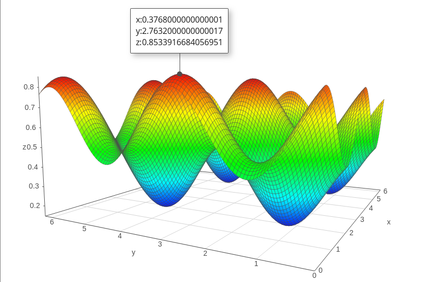 Figure 1
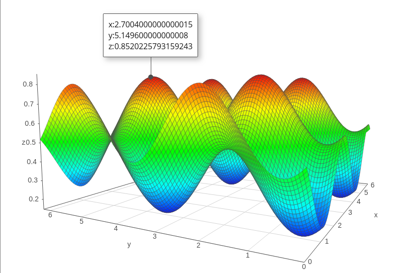 Figure 2
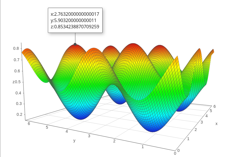 Figure 3
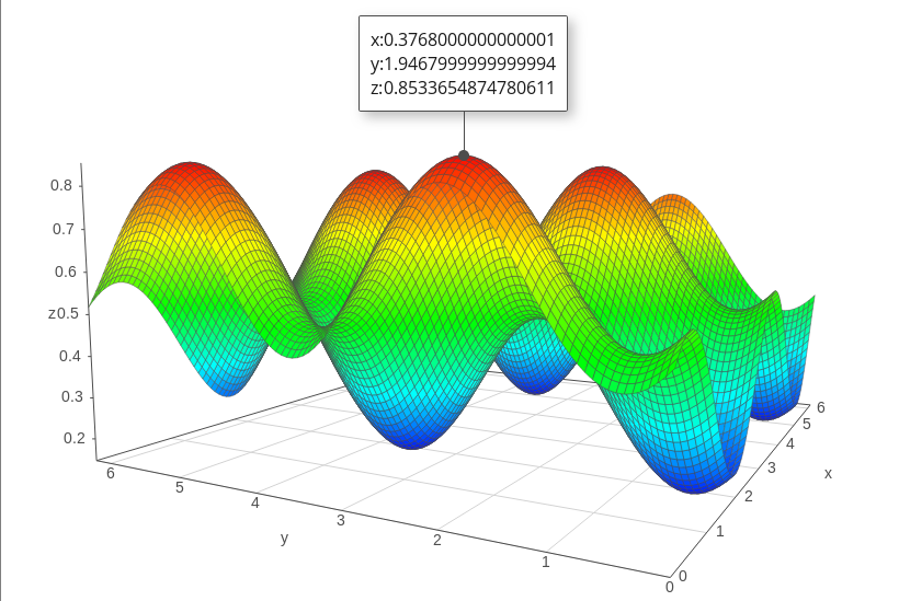 Figure 4
| LHS of winning | RHS of winning | Success | Number of such |
| condition | condition | probability | function pair |
| any non constant | XOR, XNOR | ||
| contains one | contains one | ||
| contains one | contains one | ||
| contains two | contains either | ||
| exactly one or | |||
| contains one | contains one | ||
| contains one | contains one | ||
| Any non-constant | , , |
| [0, 1, 0, 0] | [0, 1, 0, 1, 0, 0, 0, 0, 1] | ||
| [0, 1, 0, 0] | [1, 0, 0, 0, 0, 1, 0, 1, 0] | ||
| [0, 1, 1, 1] | [0, 1, 1, 1, 1, 0, 1, 0, 1] | ||
| [0, 1, 1, 1] | [1, 0, 1, 0, 1, 1, 1, 1, 0] | ||
| [1, 0, 0, 0] | [0, 1, 0, 1, 0, 0, 0, 0, 1] | ||
| [1, 0, 0, 0] | [1, 0, 0, 0, 0, 1, 0, 1, 0] | ||
| [1, 0, 1, 1] | [0, 1, 1, 1, 1, 0, 1, 0, 1] | ||
| [1, 0, 1, 1] | [1, 0, 1, 0, 1, 1, 1, 1, 0] |
| W.P. if | W.P. if | Difference | |||
|---|---|---|---|---|---|
| [0, 0, 0, 1] | [0, 1, 1, 0] | [0, 1, 0, 1, 0, 0, 0, 1, 1] | 0.85 | 0.53 | 0.32 |
| [0, 0, 0, 1] | [0, 1, 1, 0] | [0, 1, 0, 1, 0, 0, 1, 1, 1] | 0.85 | 0.51 | 0.34 |
| [0, 0, 0, 1] | [1, 0, 0, 1] | [1, 0, 1, 0, 1, 1, 1, 1, 1] | 0.85 | 0.45 | 0.4 |
| [0, 0, 1, 0] | [1, 0, 0, 1] | [1, 0, 0, 0, 1, 1, 1, 0, 1] | 0.85 | 0.41 | 0.44 |
| [0, 0, 1, 1] | [0, 1, 1, 0] | [0, 1, 0, 1, 0, 0, 0, 0, 1] | 0.85 | 0.39 | 0.46 |
| [0, 1, 0, 0] | [0, 1, 1, 0] | [0, 1, 1, 1, 0, 1, 1, 1, 1] | 0.85 | 0.42 | 0.43 |
| [0, 1, 0, 1] | [0, 1, 1, 0] | [0, 1, 1, 1, 0, 1, 0, 1, 0] | 0.85 | 0.46 | 0.39 |
| [0, 1, 1, 1] | [0, 1, 1, 0] | [0, 1, 0, 1, 0, 1, 0, 1, 0] | 0.85 | 0.45 | 0.4 |
| [1, 0, 0, 1] | [1, 0, 0, 1] | [1, 0, 1, 0, 1, 0, 1, 0, 1] | 0.85 | 0.53 | 0.32 |
| [1, 0, 1, 0] | [1, 0, 0, 1] | [1, 0, 0, 0, 1, 0, 1, 0, 1] | 0.85 | 0.46 | 0.39 |
| [1, 0, 1, 1] | [0, 1, 1, 0] | [0, 1, 0, 1, 0, 1, 0, 0, 0] | 0.85 | 0.44 | 0.41 |
| [1, 1, 0, 0] | [1, 0, 0, 1] | [1, 0, 1, 0, 1, 1, 1, 1, 0] | 0.85 | 0.39 | 0.46 |
| [1, 1, 1, 0] | [0, 1, 1, 0] | [0, 1, 1, 1, 0, 0, 0, 0, 0] | 0.85 | 0.41 | 0.44 |
| W.P. if | W.P. if | Difference | |||
|---|---|---|---|---|---|
| [0, 1, 0, 0] | [0, 1, 1, 0] | [0, 1, 0, 1, 0, 0, 0, 0, 1] | 0.46 | 0.86 | 0.4 |
| [0, 1, 0, 0] | [1, 0, 0, 0] | [1, 0, 0, 0, 0, 1, 0, 1, 0] | 0.64 | 0.86 | 0.22 |
| [0, 1, 1, 1] | [0, 1, 1, 1] | [0, 1, 1, 1, 1, 0, 1, 0, 1] | 0.63 | 0.86 | 0.23 |
| [0, 1, 1, 1] | [1, 0, 0, 1] | [1, 0, 1, 0, 1, 1, 1, 1, 0] | 0.48 | 0.86 | 0.38 |
| [1, 0, 0, 0] | [0, 1, 1, 0] | [0, 1, 0, 1, 0, 0, 0, 0, 1] | 0.48 | 0.86 | 0.38 |
| [1, 0, 0, 0] | [1, 0, 0, 0] | [1, 0, 0, 0, 0, 1, 0, 1, 0] | 0.63 | 0.86 | 0.23 |
| [1, 0, 1, 1] | [0, 1, 1, 1] | [0, 1, 1, 1, 1, 0, 1, 0, 1] | 0.64 | 0.86 | 0.22 |
| [1, 0, 1, 1] | [1, 0, 0, 1] | [1, 0, 1, 0, 1, 1, 1, 1, 0] | 0.46 | 0.86 | 0.4 |
| W.P. if | W.P. if | Difference | |||
|---|---|---|---|---|---|
| [0, 0, 0, 1] | [1, 0, 1, 1] | [1, 0, 0, 1, 1, 0, 0, 0, 0] | 0.29 | 0.76 | 0.47 |
| [0, 0, 0, 1] | [1, 0, 1, 1] | [1, 0, 0, 1, 1, 0, 0, 0, 1] | 0.29 | 0.77 | 0.48 |
| [0, 0, 0, 1] | [1, 0, 1, 1] | [1, 0, 0, 1, 1, 0, 0, 1, 0] | 0.29 | 0.77 | 0.48 |
| [0, 0, 0, 1] | [1, 0, 1, 1] | [1, 0, 0, 1, 1, 0, 0, 1, 1] | 0.29 | 0.77 | 0.48 |
| [0, 0, 0, 1] | [1, 0, 1, 1] | [1, 0, 1, 1, 1, 0, 0, 0, 0] | 0.29 | 0.76 | 0.47 |
| [0, 0, 0, 1] | [1, 0, 1, 1] | [1, 0, 1, 1, 1, 0, 0, 0, 1] | 0.29 | 0.75 | 0.46 |
| [0, 0, 0, 1] | [1, 0, 1, 1] | [1, 0, 1, 1, 1, 0, 0, 1, 0] | 0.29 | 0.77 | 0.48 |
| [0, 0, 0, 1] | [1, 0, 1, 1] | [1, 0, 1, 1, 1, 0, 0, 1, 1] | 0.29 | 0.76 | 0.47 |
| [0, 0, 1, 0] | [1, 0, 1, 1] | [1, 0, 0, 1, 1, 0, 0, 0, 0] | 0.21 | 0.76 | 0.55 |
| [0, 0, 1, 0] | [1, 0, 1, 1] | [1, 0, 0, 1, 1, 0, 0, 0, 1] | 0.21 | 0.77 | 0.56 |
| [0, 0, 1, 0] | [1, 0, 1, 1] | [1, 0, 0, 1, 1, 0, 0, 1, 0] | 0.21 | 0.77 | 0.56 |
| [0, 0, 1, 0] | [1, 0, 1, 1] | [1, 0, 0, 1, 1, 0, 0, 1, 1] | 0.21 | 0.77 | 0.56 |
| [0, 0, 1, 0] | [1, 0, 1, 1] | [1, 0, 1, 1, 1, 0, 0, 1, 1] | 0.21 | 0.76 | 0.55 |
| [0, 0, 1, 1] | [1, 0, 1, 1] | [1, 0, 0, 1, 1, 0, 0, 1, 1] | 0.36 | 0.81 | 0.45 |
| [0, 0, 1, 1] | [1, 0, 1, 1] | [1, 0, 1, 1, 1, 0, 0, 1, 1] | 0.36 | 0.84 | 0.48 |
| [1, 1, 0, 0] | [0, 1, 0, 0] | [0, 1, 0, 0, 0, 1, 1, 0, 0] | 0.36 | 0.84 | 0.48 |
| [1, 1, 0, 0] | [0, 1, 0, 0] | [0, 1, 1, 0, 0, 1, 1, 0, 0] | 0.36 | 0.81 | 0.45 |
| [1, 1, 0, 1] | [0, 1, 0, 0] | [0, 1, 0, 0, 0, 1, 1, 0, 0] | 0.21 | 0.76 | 0.55 |
| [1, 1, 0, 1] | [0, 1, 0, 0] | [0, 1, 0, 0, 0, 1, 1, 0, 1] | 0.21 | 0.77 | 0.56 |
| [1, 1, 0, 1] | [0, 1, 0, 0] | [0, 1, 0, 0, 0, 1, 1, 1, 0] | 0.21 | 0.75 | 0.54 |
| [1, 1, 0, 1] | [0, 1, 0, 0] | [0, 1, 0, 0, 0, 1, 1, 1, 1] | 0.21 | 0.76 | 0.55 |
| [1, 1, 0, 1] | [0, 1, 0, 0] | [0, 1, 1, 0, 0, 1, 1, 0, 0] | 0.21 | 0.77 | 0.56 |
| [1, 1, 0, 1] | [0, 1, 0, 0] | [0, 1, 1, 0, 0, 1, 1, 0, 1] | 0.21 | 0.77 | 0.56 |
| [1, 1, 0, 1] | [0, 1, 0, 0] | [0, 1, 1, 0, 0, 1, 1, 1, 0] | 0.21 | 0.77 | 0.56 |
| [1, 1, 0, 1] | [0, 1, 0, 0] | [0, 1, 1, 0, 0, 1, 1, 1, 1] | 0.21 | 0.76 | 0.55 |
| [1, 1, 1, 0] | [0, 1, 0, 0] | [0, 1, 0, 0, 0, 1, 1, 0, 0] | 0.29 | 0.76 | 0.47 |
| [1, 1, 1, 0] | [0, 1, 0, 0] | [0, 1, 0, 0, 0, 1, 1, 0, 1] | 0.29 | 0.77 | 0.48 |
| [1, 1, 1, 0] | [0, 1, 0, 0] | [0, 1, 0, 0, 0, 1, 1, 1, 0] | 0.29 | 0.75 | 0.46 |
| [1, 1, 1, 0] | [0, 1, 0, 0] | [0, 1, 0, 0, 0, 1, 1, 1, 1] | 0.29 | 0.76 | 0.47 |
| [1, 1, 1, 0] | [0, 1, 0, 0] | [0, 1, 1, 0, 0, 1, 1, 0, 0] | 0.29 | 0.77 | 0.48 |
| [1, 1, 1, 0] | [0, 1, 0, 0] | [0, 1, 1, 0, 0, 1, 1, 0, 1] | 0.29 | 0.77 | 0.48 |
| [1, 1, 1, 0] | [0, 1, 0, 0] | [0, 1, 1, 0, 0, 1, 1, 1, 0] | 0.29 | 0.77 | 0.48 |
| [1, 1, 1, 0] | [0, 1, 0, 0] | [0, 1, 1, 0, 0, 1, 1, 1, 1] | 0.29 | 0.76 | 0.47 |
Peer Reviews
No public reviews on file for this paper yet. If you reviewed it on a platform where reviews are public (OpenReview, ICLR, NeurIPS, ICML), you can paste yours below so the community can read it here.
Videos
No videos yet. Explain this paper in a talk, walkthrough, or lecture? Add one.
∎
11institutetext: Nayana Das 22institutetext: Applied Statistics Unit, Indian Statistical Institute, Kolkata 700108, India.
22email: [email protected] 33institutetext: Goutam Paul 44institutetext: Cryptology and Security Research Unit, R. C. Bose Centre for Cryptology and Security, Indian Statistical Institute, Kolkata 700108, India.
44email: [email protected] 55institutetext: Arpita Maitra 66institutetext: Indian Institute of Technology Kharagpur, Kharagpur 721302, India
66email: [email protected]
Dimensionality Distinguishers
Nayana Das
Goutam Paul
Arpita Maitra
Abstract
The celebrated Clauser, Horne, Shimony and Holt (CHSH) game model helps to perform the security analysis of many two-player quantum protocols. This game specifies two Boolean functions whose outputs have to be computed to determine success or failure. It also specifies the measurement bases used by each player. In this paper, we generalize the CHSH game by considering all possible non-constant Boolean functions and all possible measurement basis (up to certain precision). Based on the success probability computation, we construct several equivalence classes and show how they can be used to generate three classes of dimension distinguishers. In particular, we demonstrate how to distinguish between dimensions 2 and 3 for a special form of maximally entangled state.
Keywords:
CHSH Dimensionality testing Distinguisher Entanglement Success Probability
pacs:
03.67.−a Quantum information
1 Introduction
In quantum entanglement, two or more quantum particles (may be space-like separated) share their states in such a way that the state of each of the particles cannot be fully described without considering the other(s). If we change the quantum state of one particle thorough local unitary operations, the state of the rest of the particles changes automatically to maintain the entanglement. Many modern quantum protocols are based on entanglement theory. For example, quantum cryptography with Bell theorem eke91 , super-dense coding ben92 , quantum teleportation ben93 , entanglement swapping bose98 etc. Most of them use maximally entangled states. The Bell states are special cases of bipartite maximally entangled states on Hilbert space given by , where horo09 .
In 1935, Einstein, Podolsky and Rosen (EPR) showed that quantum mechanics is not complete eins35 . They also claimed that there may exist some local hidden variable theory, without requiring immediate action at a distance. Bell (1964) proposed a test for the existence of these hidden variables and developed an inequality bell64 and he showed that if the inequality is not satisfied, then a local hidden variable theory would not be possible. Inspired by Bell’s paper, Clauser, Horne, Shimony and Holt (CHSH) (1969) formed a correlation inequality and Bell’s theorem can be proved by using that inequality chsh69 . The CHSH inequality gives a bound on any local hidden variable model (LHVM). S. Cirel’son (1980) showed that Bell inequalities can be violated by quantum mechanical correlations cirel80 . A. Aspect, P. Grangier and G. Roger (1986) showed some experimental results, on the CHSH inequality, which agree with the quantum mechanical predictions gran86 . S. Popescu and D. Rohrlich (1994) formed some correlations, using no-signaling condition, violate the CHSH inequality even more than quantum mechanical correlations pope94 . A simple setting for showing the usefulness of entanglement involves a two-player game known as the CHSH game handout ; serg16 . Buhrman (2005) generalised the CHSH game in the field buhr05 . Some modern variants of CHSH appears in tone08 ; pawl10 ; reic13 ; brun15 ; bava15 .
1.1 Why dimensionality testing is important?
For a physical system, we generally assume that it has a particular dimension. Any practical application that uses entangled quantum systems have some predefined dimensional entangled states. In information theory, the dimensionality of quantum systems is a resource. In cryptographic applications, the security level scheme depends on the dimension. So testing dimensionality or distinguishing dimensionality of the underlying state-space are important pre-processing tasks before executing the actual protocol.
Higher dimension implies more degrees of freedom. For example, consider Quantum Key Distribution (QKD) protocol with qubit. In this case, the legitimate parties use only polarization of a photon for encoding. However, they have to fix the values for the other degrees of freedom such as spectral line, spatial mode or temporal mode etc. Lack of knowledge of any of these parameters may cause security back-door. Recently, Maitra et al. arp18 showed that if the honest party measures only the polarization of a photon and remains ignorant about the Orbital Angular Momentum (OAM), then by changing the value of OAM one can steal more information than what he/she is entitled to in a certain type of QKD protocol. This strengthens the motivation of dimensionality testing.
1.2 How to test the dimensionality?
The dimension witness gives a bound on the dimension of an unknown system based on measurement statistics. It was first introduced for quantum systems in the context of non-local correlations by Brunner et al. bru08 and further developed in Pal08 ; Per08 ; Ver10 ; Ver08 ; Jun10 ; Bri11 ; weh08 ; gal10 ; jun1 . Various experiments have been recently proposed about the implementation of such witnesses joh12 ; mar12 .
Some theory of dimensional detection of an unknown quantum system is based on the set of conditional probabilities. It is based on the analysis on the probabilities of observing an outcome after creating and measuring the system for a given set of possibilities. It has become a prominent research area in recent times weh08 ; gal10 ; jun1 . Experimental tests for testing dimension of a quantum system have been explored mar12 ; ahr12 and it has produced successful results. A simple and general dimension witnesses for quantum systems of arbitrary Hilbert space dimension was proposed by Brunner (2013) bru13 . Their proposed work can distinguish between classical and quantum systems of the same dimension. A simple method for generating nonlinear dimension witnesses for systems of arbitrary dimension has been proposed by Bowles (2014) bow14 . It has been shown in this paper that this witness can be used to certify the presence of randomness.
1.3 Our contributions
In this paper, we generalize the CHSH game and define two classes of new games which are similar to the CHSH game. The first one is for -variables and the second one is for -variables. In this class of new games we change the winning condition of the CHSH game. Instead of a particular Boolean function in the CHSH game, we use all non-constant Boolean functions and find equivalence class for function pairs and bases such that, all the elements of the same class have the same winning probability of the game. We also consider all possible measurements subject to a precision parameter. For both the games, we optimize the winning probabilities. Finally, we show how our results can be used to devise three classes of dimensionality distinguishers, particularly between dimensions 2 and 3.
The efficiency of a distinguisher depends on the number of samples (for a given success probability) and that in turn depends on the gap between the probabilities. This issue has been discussed in detail in paul18 . Moreover, there are some works basak18 on how to deal with finite number of samples. In the current work, we do not focus on these types of analysis. Rather, our main goal is to identify the distinguishing events with a significant probability gap and that is what we report here.
2 Entanglement and the CHSH game
A special type of entangled states are maximally entangled states. There are many quantum protocols which use these maximally entangled states. One of them is the CHSH game and we discuss about it.
2.1 Maximally Entangled State
Let us take a Hilbert space (for now, ). There are infinitely many maximally entangled states in and all are connected by a unitary. A pure bipartite state in is maximally entangled if the reduced density matrix is for both sub systems.
Let and . Then , where is maximally entangled as where and are reduced density matrix of subsystem A and B respectively.
Again let where and . To make , we must have .
Thus a general form of maximally entangled state in is (we are considering real coefficients only).
A maximally entangled (pure) state in a d-dimensional Hilbert space has the Schmidt decomposition in an appropriate basis. In Hilbert space (say, ), a maximally entangled (pure) state is the same as that in .
2.2 The CHSH Game
In this game there are two players, namely, Alice and Bob, and a referee. Let us assume that Alice and Bob are far away from each other and not able to communicate during the game. Before the game begins, they can communicate freely to discuss their strategy. During the game, they only communicate with the referee in the following way:
The referee chooses two independent random bits and uniformly (also called “questions”) and sends to Alice and to Bob, i.e., for all .
Alice and Bob reply to referee with bits and respectively.
Referee calculates and (where , stand for and operations respectively)
Alice and Bob win if .
Their goal is to achieve the highest winning probability together. Classically, the winning probability is . But in the quantum world, this probability is if they follow the strategy discussed in the following subsection 2.2.1.
2.2.1 Quantum Strategy
The strategy to win the game with maximum probability is to share a maximally entangled state (e.g, Bell state) between Alice and Bob. According to the referee’s questions, they choose measurement bases to measure their qubits and send their answers to the referee. Details are given in the Algorithm 1. The values of and (defined in Algorithm 1) are fixed for CHSH game and those values are , .
2.2.2 Winning Probability
Let be the event that Alice and Bob win, i.e., . Now the winning probability of the CHSH game can be written as:
[TABLE]
which again implies that for ,
[TABLE]
If the referee sends questions , Alice and Bob win if they answer identically or .
Then from Algorithm 1, the corresponding probability of winning (given ) is:
.
Similarly we have,
,
,
.
Hence from Equation (1),
[TABLE]
This probability is maximum at and the maximum value is approximately .
3 Generalized Version of the CHSH Game
We generalize the well known CHSH game to produce two types of new games. The first type of games are for -variables (i.e., each question has options to answer). The other type of games are for -variables (i.e., each question has options to answer).
Here also we assume that Alice and Bob are far away from each other and not able to communicate during the game. Before the game begins, they can communicate freely to discuss their strategy. During the game, they only communicate with the referee.
3.1 New Games for -variables (Game-1)
Our new games are similar to the CHSH game. The only exception is in the winning condition. Here the winning condition is , where and are any two variable Boolean functions other than the constant functions (the subscript in is for -variables). For variables, there are possible Boolean functions. Among them are constant functions. So we are playing this game with pairs of function where in the CHSH game there is only one pair.
3.1.1 Rules of Game-1
For a fixed pair of two variable Boolean functions we define Game-1 as follows:
The referee chooses two independent random bits and uniformly (also called “questions”) and sends to Alice and to Bob, i.e., for all .
Alice and Bob reply to referee with bits and respectively.
Referee calculates and .
Alice and Bob win if .
3.1.2 Quantum Strategy for Game-1
Alice and Bob follow the following strategy Algorithm 1 to play Game-1. Here also they share a maximally entangled state and choose measurement bases according to the referee’s questions. They measure their qubits and send their answers to the referee. Alice’s choice of measurement basis is only depends on referee’s question. But for each pair , Bob chooses the basis for which they can achieve maximum winning probability. Bob’s bases are dependent on the parameters and . So for different pairs of functions , the values of and change. For example, CHSH game is a special case of Game-1, where , , and Bob chooses and .
3.1.3 Success probabilities of Game-1
We find the success probability of the game for each and by using Equation (1), when the players follow the above strategy with changes in the chosen bases of Bob. Here Bob does not fix the value of and . For different pairs of function the value of the pair , changes as the expression of the winning probability changes.
For simplicity, we write an -variable Boolean function as a -length binary vector consisting of the last column of the truth table in lexicographical order, e.g., for a two variable function, we write and . Also LHS and RHS denote left hand side and right hand side respectively.
The results are in the following Table 1. The first two columns of Table 1 represent the functions of inputs and outputs (i.e., and )respectively, and corresponding success probabilities are given in third column. The number of such function pair having same success probabilities are in the last column.
3.1.4 Observation
From Table 1, we observe that the winning probability is maximum when and , i.e., for any non-constant variables Boolean function , if or then by playing the Game-1 we can win the game with probability .
The reason behind this is that the probability graph of these 28 cases are almost similar. To illustrate this, we show some probability graphs in Figure 1. In these graphs we plot (-axis) vs. (-axis) vs. success probability expression (-axis). From these graphs we can see that for each case the success probabilities are periodic functions of and achieve maximum value at more than one points.
The first graph in Figure 1(a) represents the success probability corresponding to the function pair and one of its maximum point is at .
The second graph in Figure 1(b) represents the success probability corresponding to the function pair and one of its maximum point is at .
The third graph in Figure 1(c) represents the success probability corresponding to the function pair , where means , and one of its maximum point is at .
The fourth graph in Figure 1(d) represents the success probability corresponding to the function pair , where means , and one of its maximum point is at .
3.2 New Games for -variables (Game-2)
In this game there are two players, namely, Alice and Bob (they are far away from each other and not able to communicate) and a referee. Let us define the sets , and .
3.2.1 Rules of Game-2
For a particular pair , where and (the subscript in is for -variables), we define Game-2 as follows:
The referee chooses two independent random bits and uniformly (also called “questions”) and sends to Alice and to Bob. That is, for all .
Alice and Bob send their answers and () to the referee.
Referee calculates and .
Alice and Bob win if .
3.2.2 Quantum Strategy for Game-2
Now let Alice and Bob play the game with the following strategy given in Algorithm 2. Before the game starts, they share a maximally entangled bipartite state: in the Hilbert space . According to the referee’s questions, they choose measurement bases to measure their qubits and send their answers to the referee. Alice’s choice of measurement basis is only depends on referee’s question. But for each pair , Bob choose the basis for which they can achieve maximum winning probability. Bob’s bases are dependent on the parameters and .
3.2.3 Example of Game-2
Let us take an example. Let and (i.e., ). If we play the above game with these and then the success probability is at .
3.2.4 Maximum Winning Probability
In this Game-2 the maximum winning probability is only for pairs of function .
Now the function pairs, with the highest winning probability and corresponding bases are shown in Table 2.
3.3 Equivalence Classes
From the results of these two games we observe that, if we introduce some equivalence relations to make partition of the set of data in each game result, then we will take only one element of each equivalence class to play these games. It will reduce the time and space complexity of these games. Also if some measurement setup will be unavailable then we can use any other setup from the same class to continue the games. Here we take three equivalence relations to make three different types of partitions of the results.
We can make an equivalence class of the bases of Bob for a fixed function pair , (), such that all elements of the same class give the same success probability.
For simplicity, we only write the value of the pair as a basis (i.e., we represent a basis as a point in ) in a class and we take the values in (i.e., ) and as a multiple of .
For example, if we fix and in Game-1, then there are equivalence classes of bases (up to significant digit). Now in the previous example, if we consider the success probabilities up to significant digits, then there are elements in the class of highest winning probability and the class is
[TABLE]
Again in Game-2, let and (i.e. ) , then there are equivalence classes of bases (up to significant digit). Now in the previous example, if we consider the success probabilities up to significant digits, then there are elements in the class of highest winning probability and the class is
[TABLE] 2. 2.
Secondly, we fix the bases of Bob and vary the function pairs to make the equivalence classes. Here also all the elements of the same class have the same winning probability.
For example, in Game-1, if we fix , then , , , etc. are all belong to the same class with success probability . 3. 3.
At last, we vary both function pairs and Bob’s bases and the tuples which have the same winning probability are belong to the same class. E.g., in Game-2, each row of Table 2 have the same success probability and thus they belong to the same class.
4 Dimensionality Testing
We observe the winning probabilities of various cases in Game-1 and Game-2.
By using the above two games we can make device independent dimension distinguisher to distinguish between the states and . For example,
In Game-1, if we take and and , , then the winning probability of this game is .
In Game-2, if we take and and , , then winning probability of this game is .
So by playing these games and observing winning probabilities we can easily distinguish between and . In other words, we can say the dimension of the given maximally state is two or three.
We can think this whole process as a union of two black boxes. An initial black box is the state preparatory which prepares states of form either or . the prepared state is then sent to a second black box, the measurement device. In this box, if the states are , it will follow the process of Game-1 and if the states are , it will follow the process of Game-2.
From the outputs of this measurement device we will calculate the winning probability of the game played in this box and compare this probability with the success probabilities of Game-1 and Game-2. So we have a dimension distinguisher. The protocol is described in Algorithm 3.
Following the above process and by changing the function pairs in the games we can find many distinguishers. For each, we use the function pair in Game-2 and the function pair in Game-1 (where, is the restriction of in variables, i.e., ). We divide the set of all distinguisher into classes according to the winning probabilities of the games.
4.1 First class of distinguishers ()
In this set, we put all the distinguishers where we choose function pairs such that the function pair has the highest winning probability in Game-1 (i.e., ) which is greater than the winning probability of the corresponding Game-2.
If we choose , thus (or , thus ), then the winning probabilities of the Game-1 and Game-2 are and . Therefore the difference of these probabilities is , which is quite good.
There are many distinguishers in this class. We put some of them into the following Table 3. Here we take the winning probability for at that point where the corresponding winning probability for is maximum.
4.2 Second class of distinguishers ()
In this set, we put all the distinguishers where we choose function pairs such that it has the highest winning probability in Game-2 (i.e., ) which is greater than the winning probability of corresponding Game-1 with function pair . Here we take the winning probability for at that point where the corresponding winning probability for is maximum.
For example, let then if success probability is and if success probability is . We put all distinguishers in Table 4.
4.3 Third class of distinguishers ()
Similarly, we can make dimension distinguisher using other function pairs for which the difference between the optimal winning probabilities of the two games is non-negligible. Here we take function pair and corresponding pair such that both the games with respective pairs do not achieve the highest winning probabilities. we put all these distinguishers in this set. The cardinality of this set depends on the difference value between winning probabilities.
Let be a function pair and the highest winning probability of Game-2 with being at point and the same of Game-1 with is at point . We compare , and take the best (say, ). Then we find the winning probability of Game-2 at and difference value . We make a list of these distinguishers for which the difference value is greater than in Table 5.
5 Conclusion
Dimensionality of the states act as a resource in quantum information processing tasks. For many protocols, the performance as well as security depends on the particular value of the dimension. For this reason, dimensionality testing is very important. There have been several works on dimension witness. We take a different route by constructing dimension distinguishers based on our generalized version of the the CHSH game. We demonstrate several classes of practical distinguishers between 2 and 3 dimensions.
The reference list from the paper itself. Each links out to its DOI / PubMed record.
- 1(1) Ekert, A.K.: Quantum cryptography based on Bell’s theorem. Phys. Rev. Lett., 67 , 661 (1991)
- 2(2) Bennett, C. H., Wiesner, S. J.: Communication via one-and two-particle operators on Einstein-Podolsky-Rosen states. Phys. Rev. Lett., 69(20) , 2881 (1992)
- 3(3) Bennett, C. H., Brassard, G., Crépeau, C., Jozsa, R., Peres, A., Wootters, W. K.: Teleporting an unknown quantum state via dual classical and Einstein-Podolsky-Rosen channels. Phys. Rev. Lett., 70(13) , 1895 (1993)
- 4(4) Bose, S., Vedral, V., Knight, P. L.: Multiparticle generalization of entanglement swapping. Phys. Rev. A, 57(2) , 822 (1998)
- 5(5) Horodecki, R., Horodecki, P., Horodecki, M., Horodecki, K.: Quantum entanglement. Rev. Mod. Phys., 81(2) , 865 (2009)
- 6(6) Einstein, A., Podolsky, B., Rosen, N.: Can quantum-mechanical description of physical reality be considered complete?. Phys. Rev., 47(10) , 777 (1935)
- 7(7) Bell, J. S.: On the einstein podolsky rosen paradox. Physics Physique Fizika, 1(3) , 195 (1964)
- 8(8) Clauser, J. F., Horne, M. A., Shimony, A., Holt, R. A.: Proposed experiment to test local hidden-variable theories. Phys. Rev. Lett., 23(15) , 880 (1969)