Flow organization and heat transfer in turbulent wall sheared thermal convection
Alexander Blass, Xiaojue Zhu, Roberto Verzicco, Detlef Lohse, Richard, J.A.M. Stevens

TL;DR
This study uses direct numerical simulations to explore how wall shear influences flow organization and heat transfer in turbulent Rayleigh-Bénard convection across different regimes, revealing transitions from buoyancy to shear dominance.
Contribution
It identifies three distinct flow regimes in wall-sheared thermal convection and characterizes their flow structures and heat transfer scaling behaviors.
Findings
Heat transfer decreases then increases with shear at fixed Ra.
Flow transitions from buoyancy-driven to shear-dominated structures.
Nusselt number scaling varies across regimes, with different exponents.
Abstract
We perform direct numerical simulations of wall sheared Rayleigh-B\'enard (RB) convection for Rayleigh numbers up to , Prandtl number unity, and wall shear Reynolds numbers up to . Using the Monin-Obukhov length we identify three different flow states, a buoyancy dominated regime (; with the thermal boundary layer thickness), a transitional regime (; with the height of the domain), and a shear dominated regime (). In the buoyancy dominated regime the flow dynamics are similar to that of turbulent thermal convection. The transitional regime is characterized by rolls that are increasingly elongated with increasing shear. The flow in the shear dominated regime consists of very large-scale meandering rolls, similar to the ones found in…
Click any figure to enlarge with its caption.
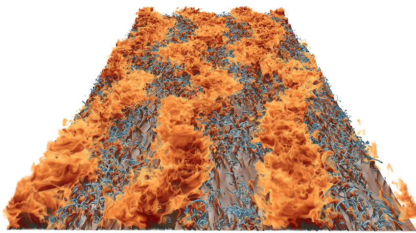 Figure 1
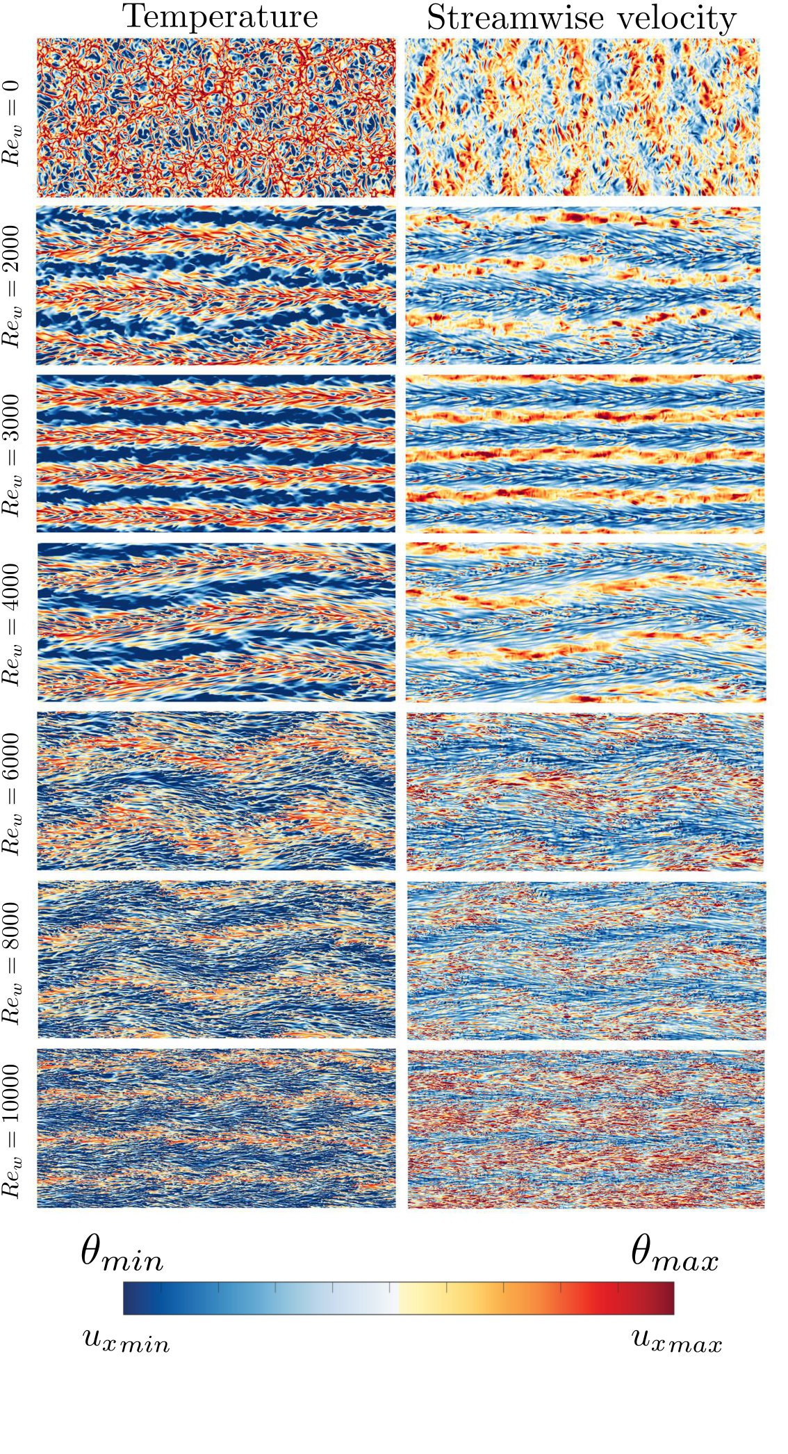 Figure 10
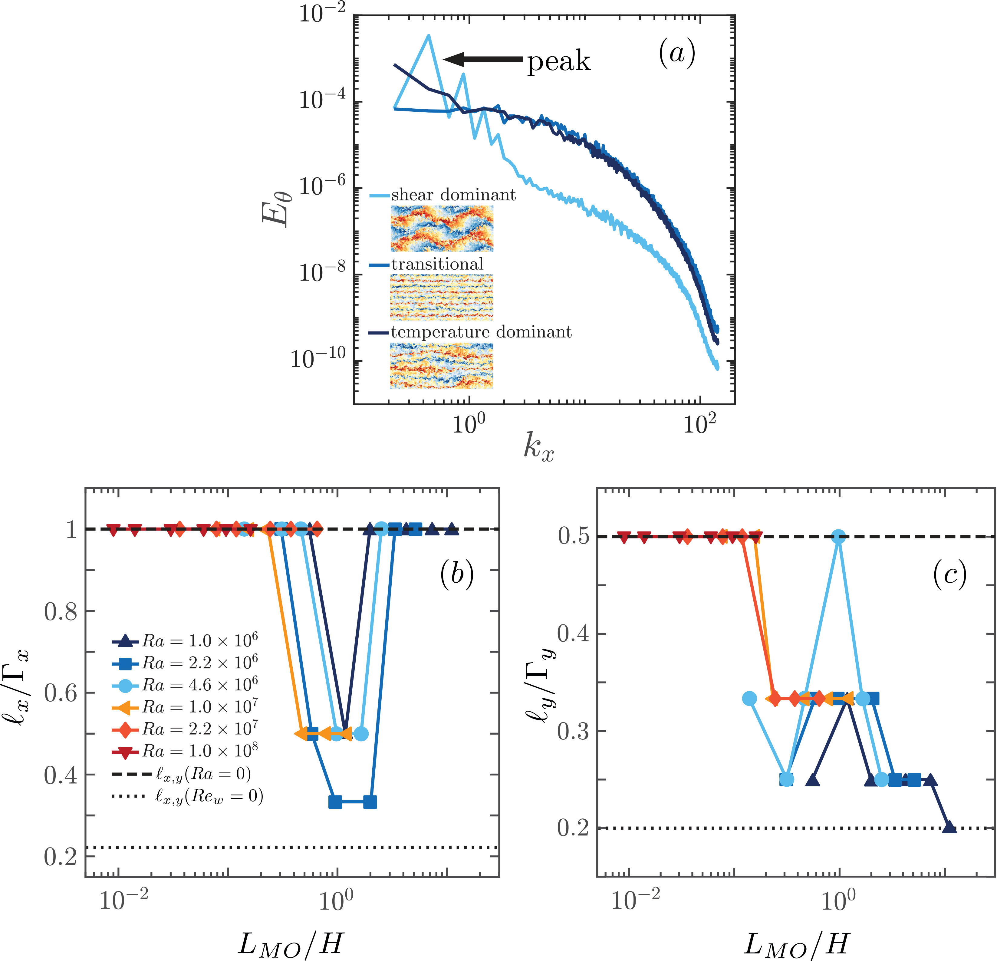 Figure 11
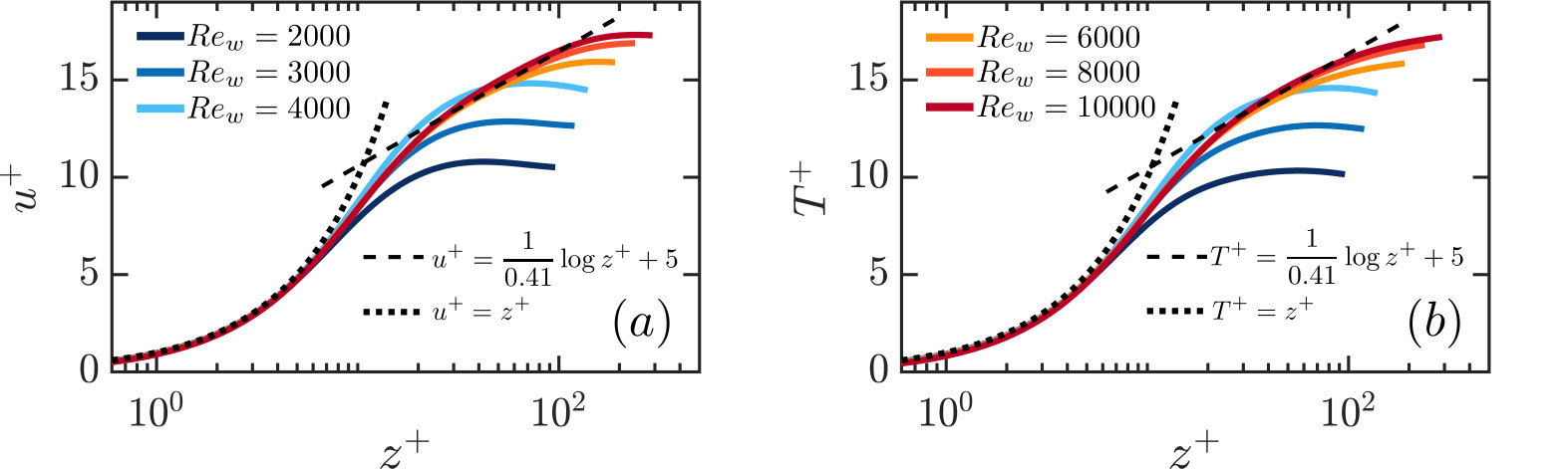 Figure 12
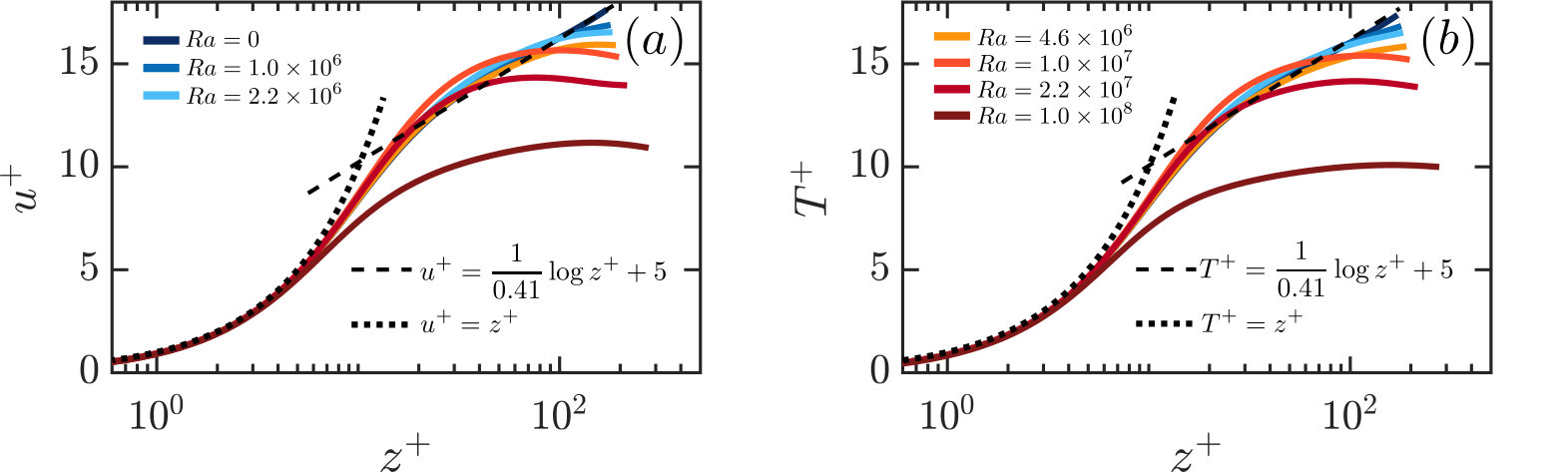 Figure 13
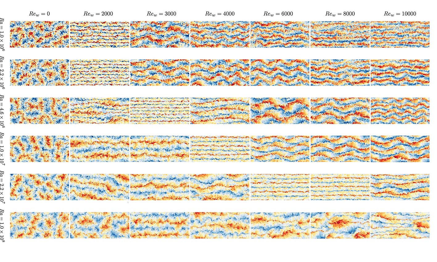 Figure 14
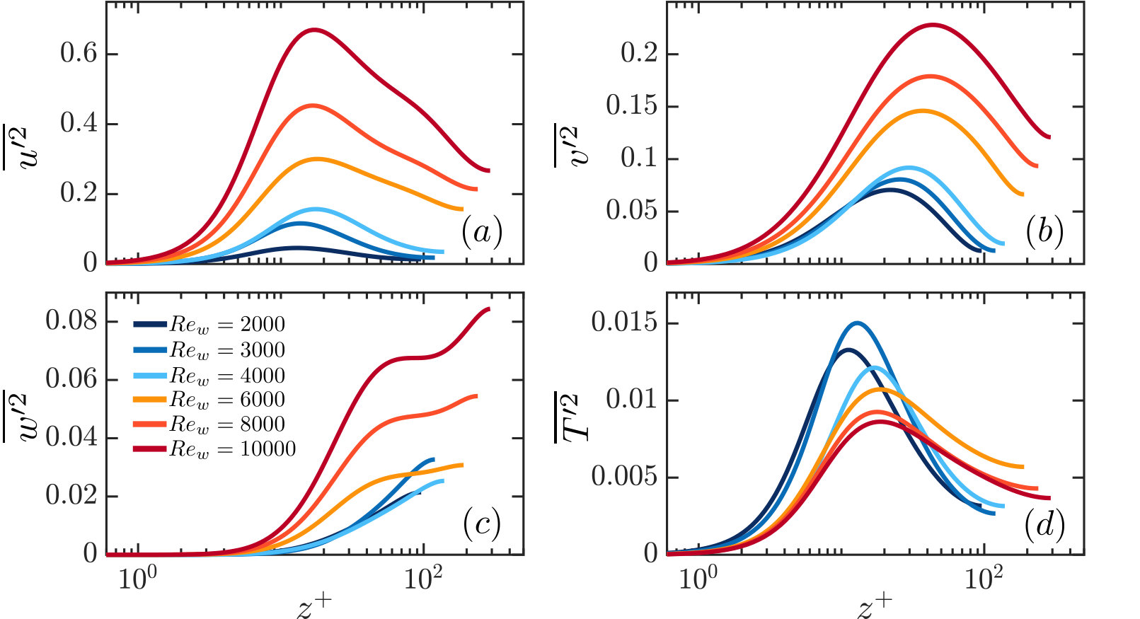 Figure 15
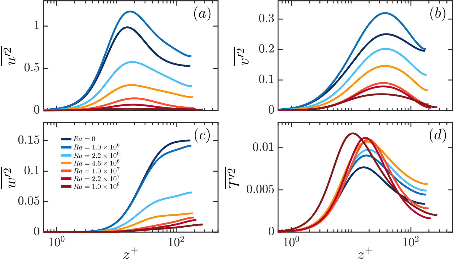 Figure 16
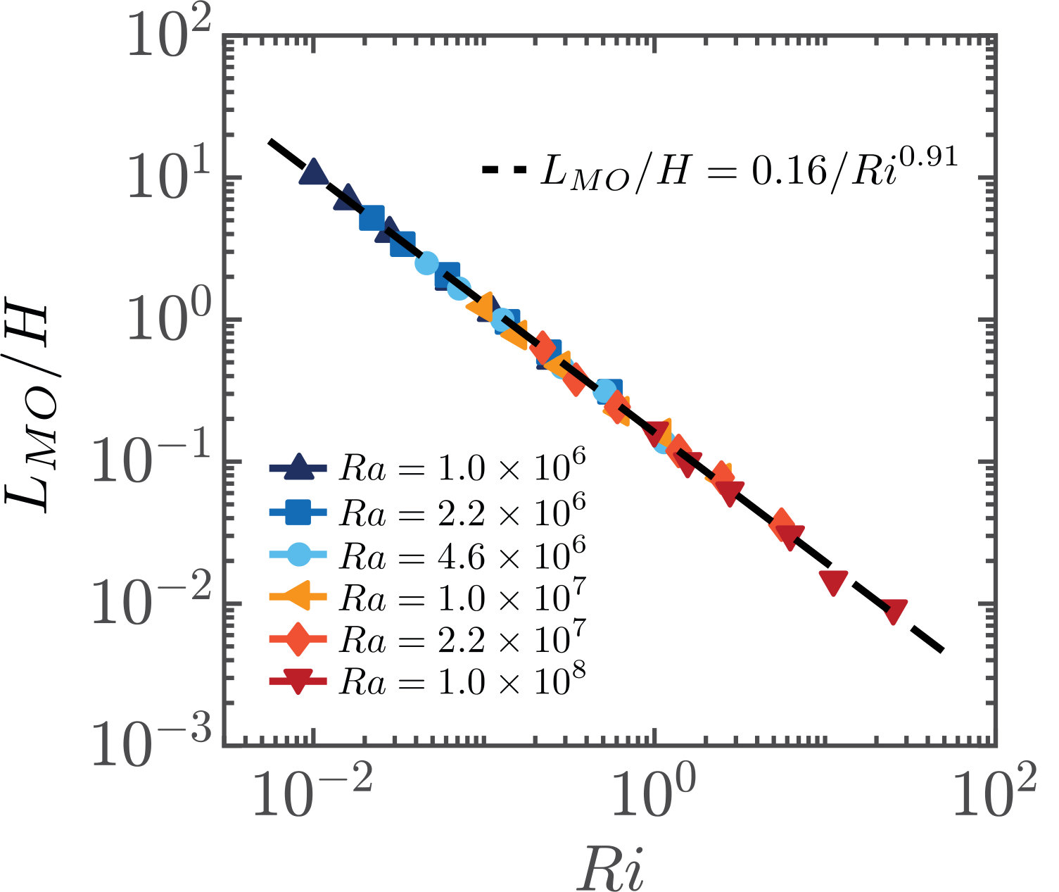 Figure 17
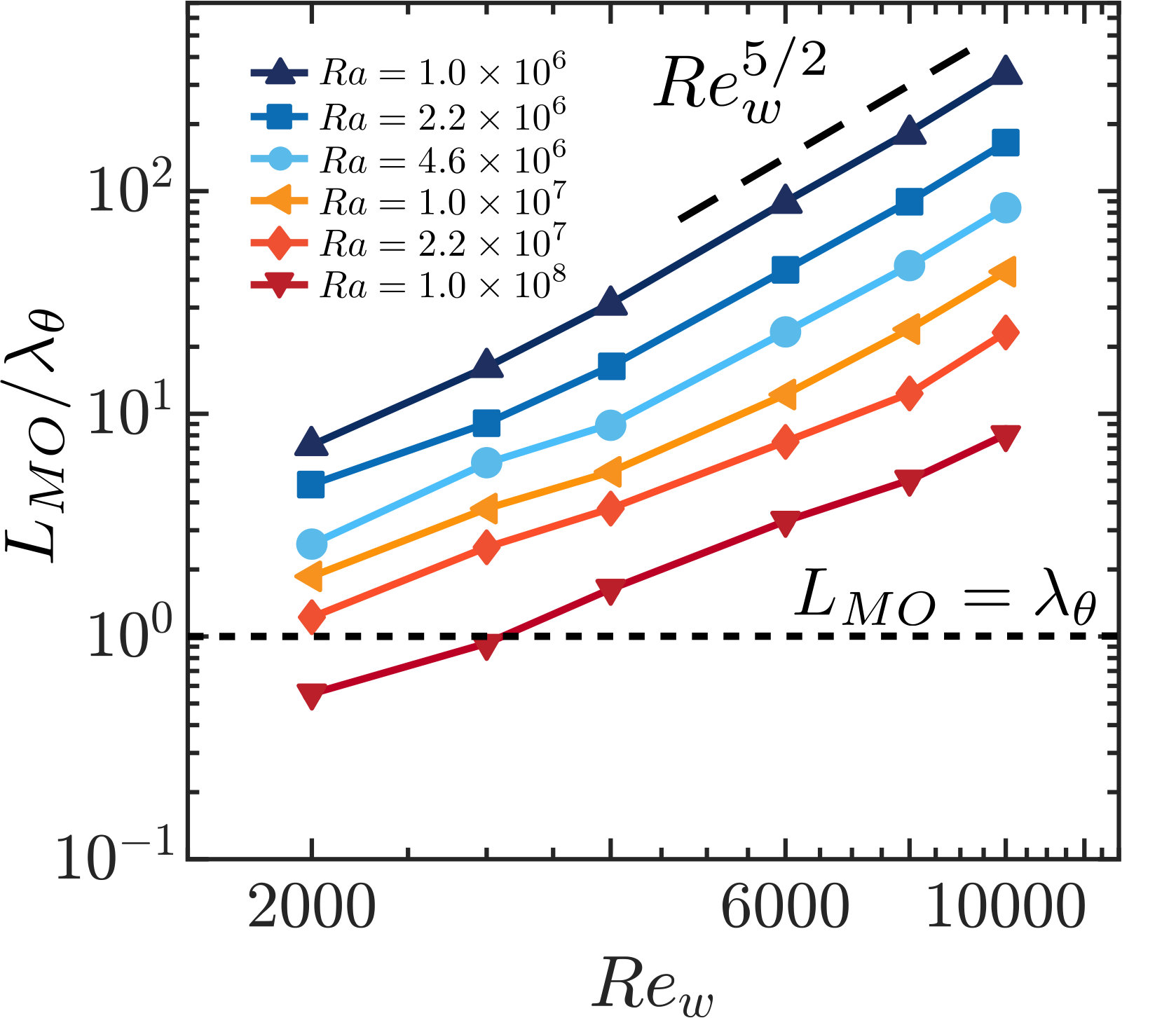 Figure 18
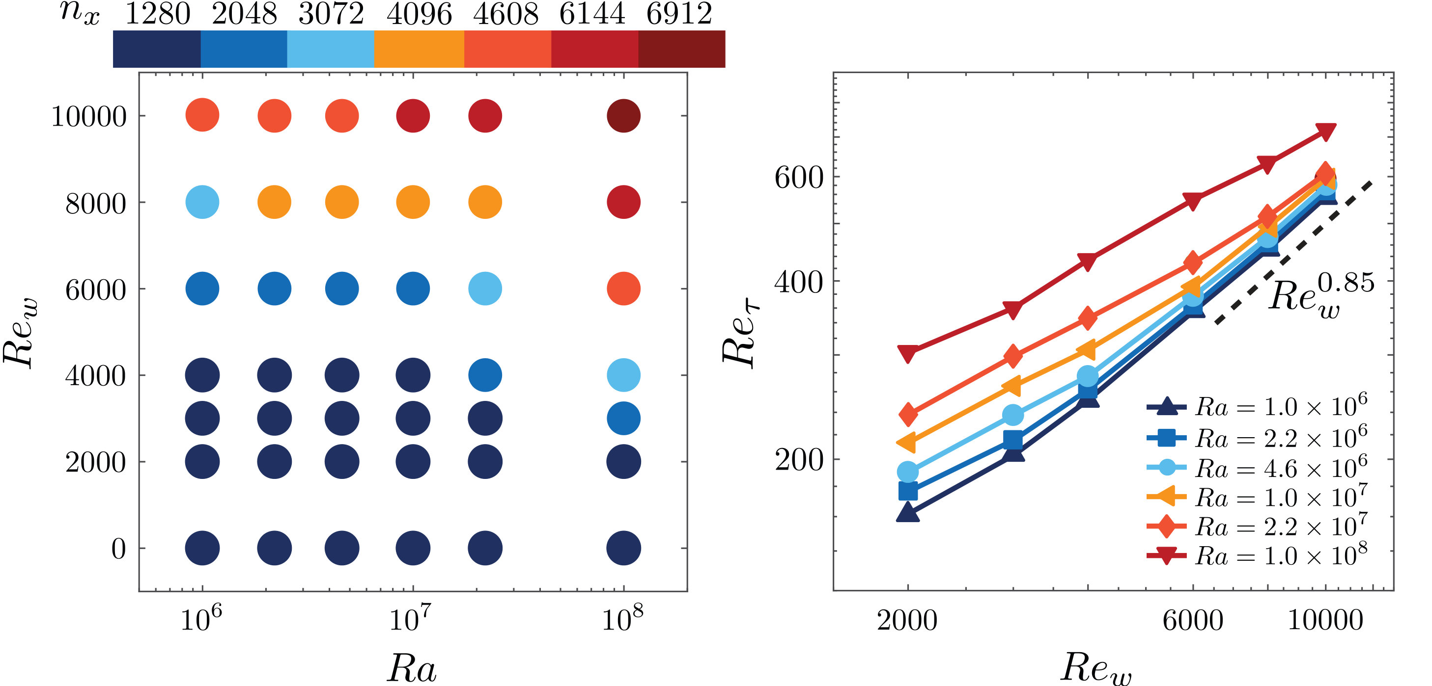 Figure 2
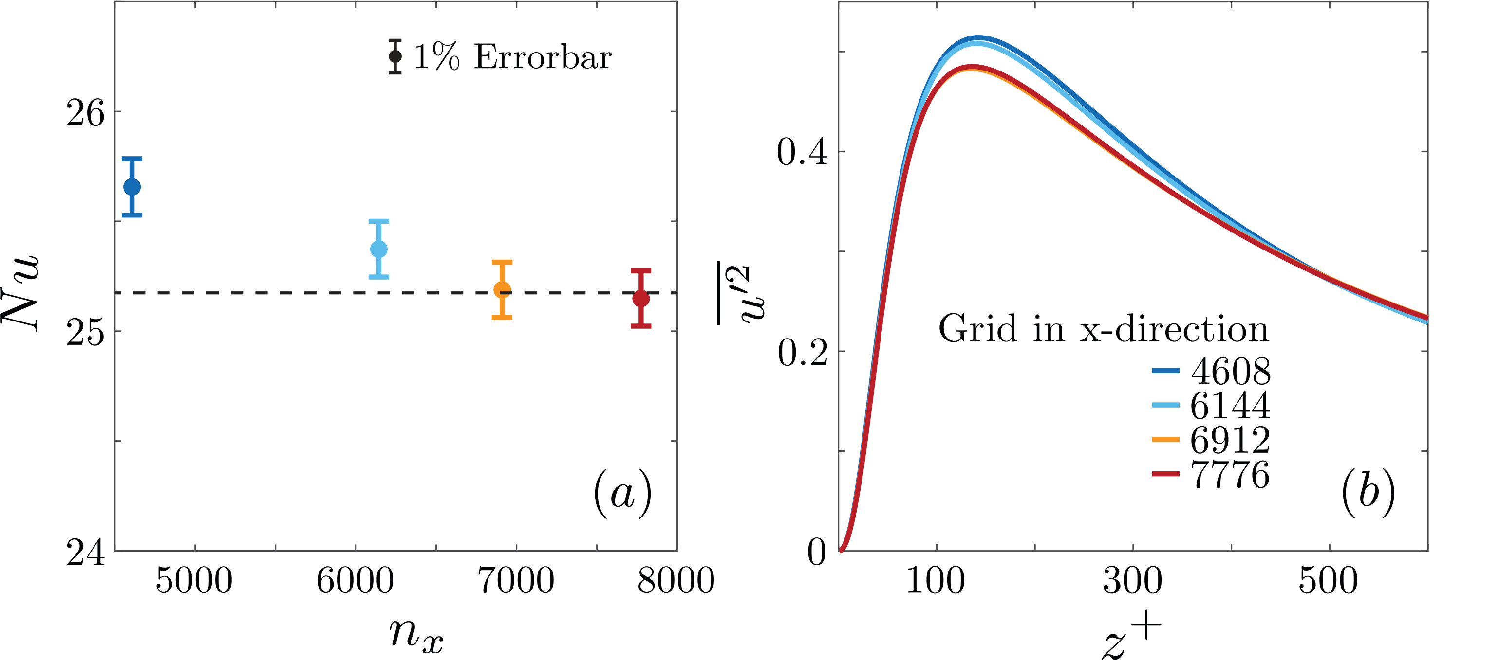 Figure 3
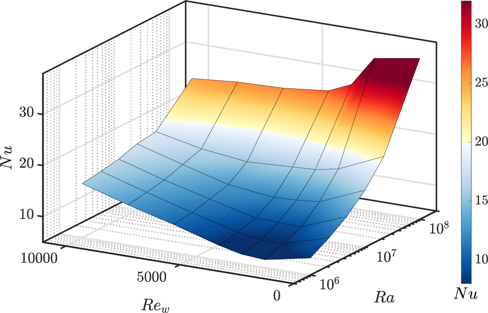 Figure 4
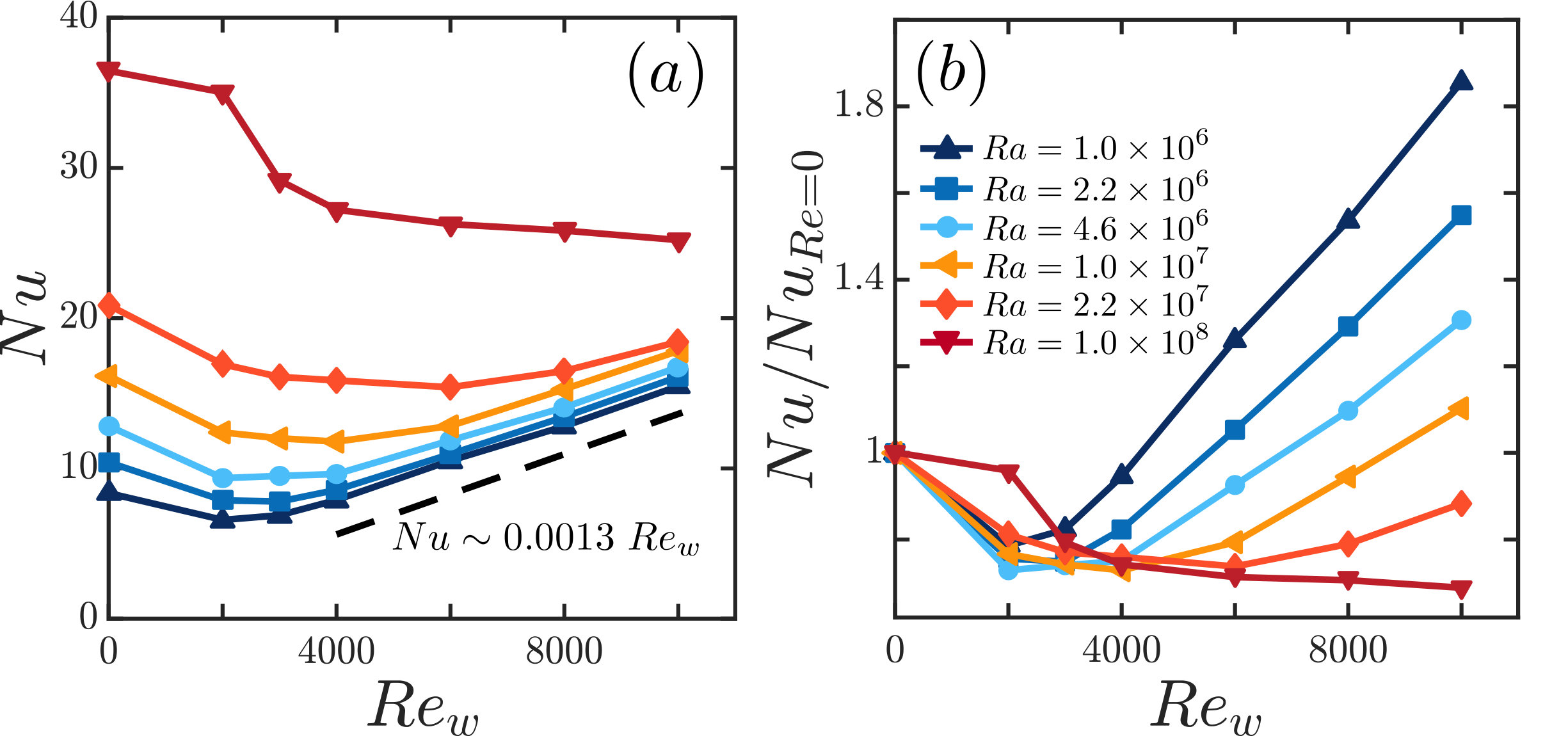 Figure 5
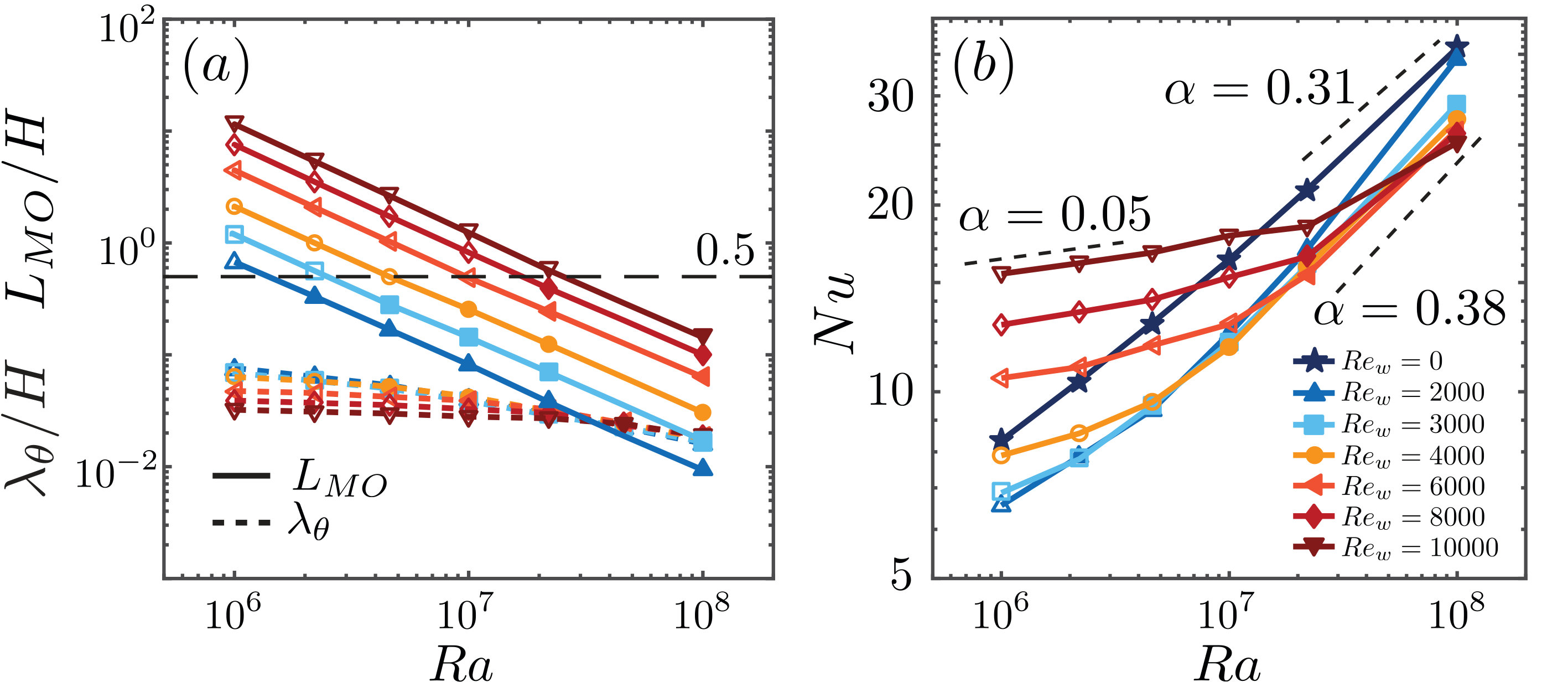 Figure 6
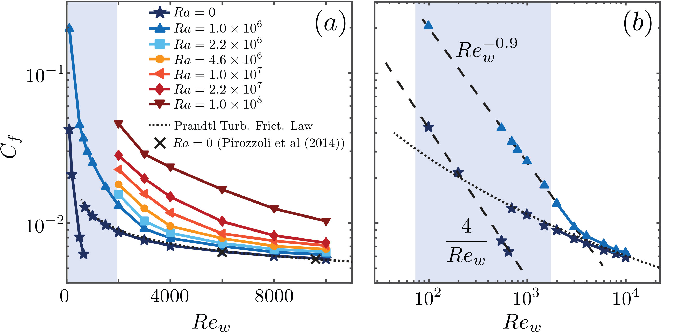 Figure 7
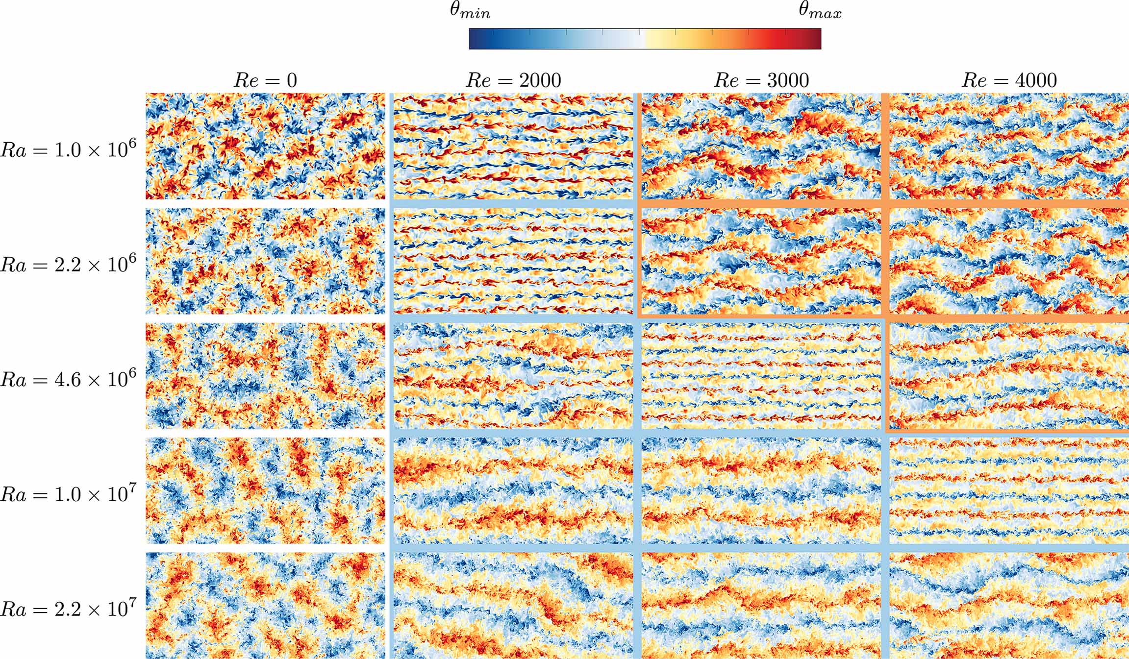 Figure 8
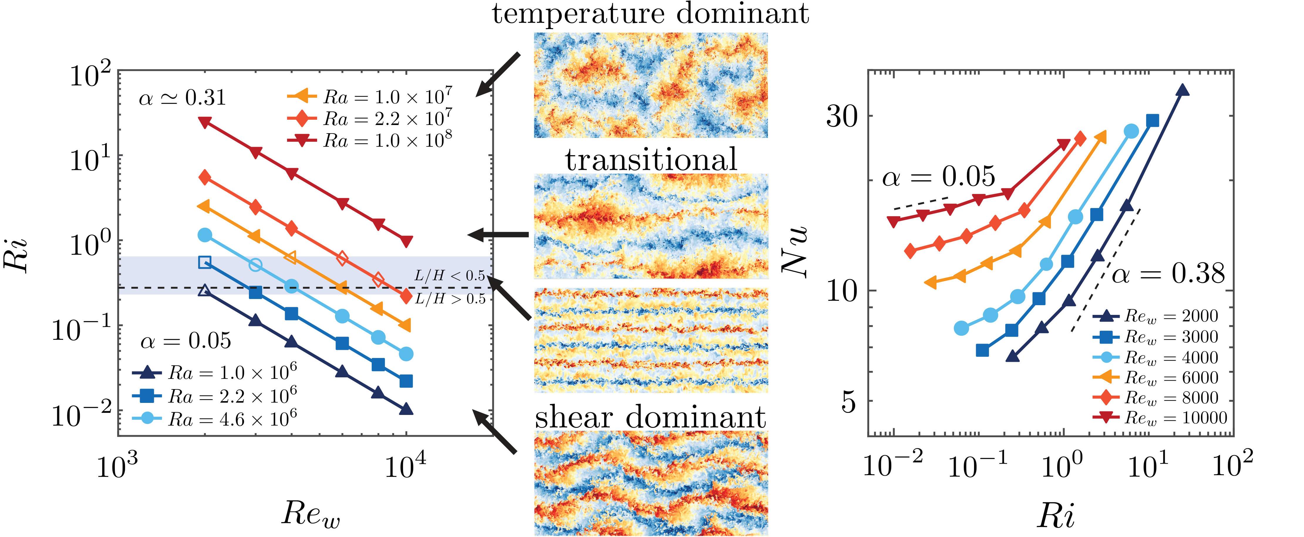 Figure 9
| 1 | 10000 | 1024 | 512 | 384 | 708.0 | 1.000 | 0.138 | 25.66 | 10.03 | ||||
| 1 | 10000 | 1296 | 648 | 384 | 703.6 | 1.000 | 0.137 | 25.37 | 9.902 | ||||
| 1 | 10000 | 1536 | 768 | 384 | 700.6 | 1.000 | 0.137 | 25.19 | 9.818 | ||||
| 1 | 10000 | 1728 | 864 | 384 | 700.0 | 1.000 | 0.136 | 25.15 | 9.805 |
| 1 | 2000 | 1280 | 1024 | 256 | 134.0 | 0 | 0 | 0 | 8.971 | ||||
| 1 | 3000 | 1280 | 1024 | 256 | 188.7 | 0 | 0 | 0 | 7.917 | ||||
| 1 | 4000 | 1280 | 1024 | 256 | 241.8 | 0 | 0 | 0 | 7.314 | ||||
| 1 | 6000 | 1280 | 1024 | 256 | 346.0 | 0 | 0 | 0 | 6.651 | ||||
| 1 | 8000 | 2048 | 1280 | 256 | 400.8 | 0 | 0 | 0 | 5.020 | ||||
| 1 | 10000 | 3072 | 1536 | 256 | 468.0 | 0 | 0 | 0 | 4.382 | ||||
| 1 | 0 | 1280 | 1024 | 256 | 0 | 0 | 8.343 | ||||||
| 1 | 2000 | 1280 | 1024 | 256 | 164.2 | 0.250 | 0.552 | 6.557 | 13.49 | ||||
| 1 | 3000 | 1280 | 1024 | 256 | 206.2 | 0.111 | 1.180 | 6.869 | 9.449 | ||||
| 1 | 4000 | 1280 | 1024 | 256 | 255.7 | 0.063 | 1.983 | 7.891 | 8.173 | ||||
| 1 | 6000 | 2048 | 1280 | 256 | 360.7 | 0.028 | 4.258 | 10.52 | 7.231 | ||||
| 1 | 8000 | 3072 | 1536 | 256 | 459.3 | 0.016 | 7.211 | 12.82 | 6.592 | ||||
| 1 | 10000 | 4608 | 2304 | 320 | 563.0 | 0.010 | 11.00 | 15.49 | 6.340 | ||||
| 1 | 0 | 1280 | 1024 | 256 | 0 | 0 | 10.40 | ||||||
| 1 | 2000 | 1280 | 1024 | 256 | 179.0 | 0.550 | 0.306 | 7.866 | 16.03 | ||||
| 1 | 3000 | 1280 | 1024 | 256 | 218.7 | 0.244 | 0.582 | 7.788 | 10.63 | ||||
| 1 | 4000 | 1280 | 1024 | 256 | 266.1 | 0.138 | 0.953 | 8.568 | 8.848 | ||||
| 1 | 6000 | 2048 | 1280 | 256 | 368.7 | 0.061 | 2.021 | 10.96 | 7.551 | ||||
| 1 | 8000 | 4096 | 2048 | 256 | 470.0 | 0.034 | 3.350 | 13.44 | 6.904 | ||||
| 1 | 10000 | 4608 | 2304 | 320 | 575.3 | 0.022 | 5.123 | 16.12 | 6.619 | ||||
| 1 | 0 | 1280 | 1024 | 256 | 0 | 0 | 12.83 | ||||||
| 1 | 2000 | 1280 | 1024 | 256 | 193.2 | 1.150 | 0.139 | 9.353 | 18.66 | ||||
| 1 | 3000 | 1280 | 1024 | 256 | 241.0 | 0.511 | 0.316 | 9.502 | 12.91 | ||||
| 1 | 4000 | 1280 | 1024 | 256 | 280.4 | 0.288 | 0.466 | 9.626 | 9.829 | ||||
| 1 | 6000 | 2048 | 1280 | 256 | 383.1 | 0.128 | 0.982 | 11.88 | 8.154 | ||||
| 1 | 8000 | 4096 | 2048 | 256 | 481.5 | 0.072 | 1.644 | 14.08 | 7.244 | ||||
| 1 | 10000 | 4608 | 2304 | 320 | 587.7 | 0.046 | 2.512 | 16.76 | 6.910 | ||||
| 1 | 0 | 1280 | 1024 | 256 | 0 | 0 | 16.18 | ||||||
| 1 | 2000 | 1280 | 1024 | 256 | 216.5 | 2.500 | 0.075 | 12.41 | 23.45 | ||||
| 1 | 3000 | 1280 | 1024 | 256 | 269.9 | 1.111 | 0.156 | 12.02 | 16.19 | ||||
| 1 | 4000 | 1280 | 1024 | 256 | 310.7 | 0.625 | 0.233 | 11.78 | 12.07 | ||||
| 1 | 6000 | 2048 | 1280 | 256 | 397.3 | 0.278 | 0.475 | 12.85 | 8.771 | ||||
| 1 | 8000 | 4096 | 2048 | 256 | 501.1 | 0.156 | 0.785 | 15.30 | 7.848 | ||||
| 1 | 10000 | 6144 | 3072 | 320 | 604.3 | 0.100 | 1.218 | 17.85 | 7.305 | ||||
| 1 | 0 | 1280 | 1024 | 256 | 0 | 0 | 20.92 | ||||||
| 1 | 2000 | 1280 | 1024 | 256 | 241.4 | 5.500 | 0.036 | 16.97 | 29.15 | ||||
| 1 | 3000 | 1280 | 1024 | 256 | 302.9 | 2.445 | 0.078 | 16.13 | 20.40 | ||||
| 1 | 4000 | 2048 | 1280 | 256 | 351.1 | 1.375 | 0.118 | 15.90 | 15.42 | ||||
| 1 | 6000 | 3072 | 1536 | 256 | 435.8 | 0.611 | 0.243 | 15.43 | 10.56 | ||||
| 1 | 8000 | 4096 | 2048 | 256 | 522.0 | 0.344 | 0.374 | 16.52 | 8.517 | ||||
| 1 | 10000 | 6144 | 3072 | 320 | 613.9 | 0.220 | 0.644 | 18.01 | 7.541 | ||||
| 1 | 0 | 1280 | 1024 | 256 | 0 | 0 | 36.52 | ||||||
| 1 | 2000 | 1280 | 1024 | 256 | 307.2 | 25.00 | 0.009 | 35.06 | 47.20 | ||||
| 1 | 3000 | 2048 | 1280 | 256 | 365.5 | 11.11 | 0.014 | 29.18 | 29.68 | ||||
| 1 | 4000 | 3072 | 1536 | 256 | 440.6 | 6.250 | 0.030 | 27.23 | 24.27 | ||||
| 1 | 6000 | 4608 | 2304 | 320 | 557.0 | 2.778 | 0.060 | 26.27 | 17.24 | ||||
| 1 | 8000 | 6144 | 3072 | 320 | 660.6 | 1.563 | 0.097 | 26.00 | 13.64 | ||||
| 1 | 10000 | 6912 | 3456 | 384 | 740.2 | 1.000 | 0.160 | 25.21 | 10.96 |
Peer Reviews
No public reviews on file for this paper yet. If you reviewed it on a platform where reviews are public (OpenReview, ICLR, NeurIPS, ICML), you can paste yours below so the community can read it here.
Videos
No videos yet. Explain this paper in a talk, walkthrough, or lecture? Add one.
Flow organization and heat transfer in turbulent wall sheared thermal convection
Alexander Blass\aff1 \corresp
Xiaojue Zhu\aff1,2
Roberto Verzicco\aff3,1,4
Detlef Lohse\aff1,5
Richard J.A.M. Stevens\aff1 \corresp
\aff1 Physics of Fluids Group, Max Planck Center for Complex Fluid Dynamics, J. M. Burgers Center for Fluid Dynamics and MESA+ Research Institute, Department of Science and Technology, University of Twente, P.O. Box 217, 7500 AE Enschede, The Netherlands \aff2 Center of Mathematical Sciences and Applications, School of Engineering and Applied Sciences, Harvard University, Cambridge, MA 02138, USA \aff3 Dipartimento di Ingegneria Industriale, University of Rome ”Tor Vergata”. Via del Politecnico 1, Roma 00133, Italy \aff4 Gran Sasso Science Institute - Viale F. Crispi, 7 67100 L’Aquila, Italy. \aff5 Max Planck Institute for Dynamics and Self-Organization, Am Fassberg 17, 37077 Göttingen, Germany
Abstract
We perform direct numerical simulations of wall sheared Rayleigh-Bénard (RB) convection for Rayleigh numbers up to , Prandtl number unity, and wall shear Reynolds numbers up to . Using the Monin-Obukhov length we identify three different flow states, a buoyancy dominated regime (; with the thermal boundary layer thickness), a transitional regime (; with the height of the domain), and a shear dominated regime (). In the buoyancy dominated regime the flow dynamics are similar to that of turbulent thermal convection. The transitional regime is characterized by rolls that are increasingly elongated with increasing shear. The flow in the shear dominated regime consists of very large-scale meandering rolls, similar to the ones found in conventional Couette flow. As a consequence of these different flow regimes, for fixed and with increasing shear, the heat transfer first decreases, due to the breakup of the thermal rolls, and then increases at the beginning of the shear dominated regime. For the Nusselt number effectively scales as , with while we find in the buoyancy dominated regime. In the transitional regime the effective scaling exponent is , but the temperature and velocity profiles in this regime are not logarithmic yet, thus indicating transient dynamics and not the ultimate regime of thermal convection.
1 Introduction
Rayleigh-Bénard (RB) convection, i.e. the flow in a box heated from below and cooled from above, is one of the paradigmatic fluid dynamical systems (Ahlers et al., 2009; Lohse & Xia, 2010; Chilla & Schumacher, 2012; Xia, 2013). The dynamics of RB convection are controlled by the Rayleigh number
[TABLE]
which is the non-dimensional temperature difference between the horizontal plates, and the Prandtl number
[TABLE]
which is the ratio of momentum and thermal diffusivities. In equations (1) and (2), is the non-dimensional distance between the plates, the thermal expansion coefficient of the fluid, the gravitational acceleration, the temperature difference between top and bottom plate, and and the thermal and kinetic diffusivities, respectively. The crucial additional control parameter, whose effect we will analyse in this paper, is the wall shear Reynolds number
[TABLE]
with the velocity of the wall. The ratio between buoyancy and shear driving can be expressed as bulk Richardson number
[TABLE]
which can be seen as alternative control parameter for either or .
Important responses of the system are the Nusselt number
[TABLE]
which is the dimensionless vertical heat flux, the friction Reynolds number
[TABLE]
and the skin friction coefficient
[TABLE]
Here is the constant vertical heat flux, with and the fluctuations for wall-normal velocity and temperature, respectively, and the friction velocity, with the mean wall shear stress and the density of the fluid.
For strong enough thermal driving, i.e. high enough , the flow in the bulk region becomes fully turbulent. For even stronger thermal driving, beyond some critical number , also the boundary layers become turbulent and the system reaches the regime of so-called ultimate convection (Kraichnan, 1962; Grossmann & Lohse, 2000, 2001, 2011). This ultimate regime sets in when the shear Reynolds number at the boundary layers is sufficiently high so that the boundary layer becomes turbulent, leading to a strong increase in the heat transport, quantified by the Nusselt number.
Ahlers et al. (2012) found that the transition to the ultimate regime sets in around . While in the classical regime one generally finds , in the ultimate regime , in agreement with theoretical predictions (Grossmann & Lohse, 2011).
The transition to the ultimate regime has also been observed in direct numerical simulations (DNS) of two-dimensional RB convection (Zhu et al., 2018a). In Taylor-Couette flow, which is a very analogous system, experiments and DNS have observed the ultimate regime as well (Grossmann et al., 2016). Such scaling has also been observed in experiments with vertical pipes (Gibert et al., 2006; Cholemari & Arakeri, 2009; Pawar & Arakeri, 2016). However, so far the ultimate regime has not yet been achieved in DNS of three-dimensional RB flows (Stevens et al., 2010, 2011) as the required computational time to achieve this is still out of reach. In an attempt to trigger the transition to the ultimate regime, here we add a Couette type shearing to the RB system to increase the shear Reynolds number of the boundary layers.
In Couette flow the top and bottom walls move in opposite directions (Thurlow & Klewicki, 2000; Barkley & Tuckerman, 2005; Tuckerman & Barkley, 2011) with constant and just as in other examples of wall bounded turbulence (Jiménez, 2018; Smits et al., 2011; Smits & Marusic, 2013) the flow is dominated by elongated streaks, which have been observed in experiments (Kitoh & Umeki, 2008) and DNS (Lee & Kim, 1991; Tsukahara et al., 2006), even at relatively low shear Reynolds numbers (Chantry et al., 2017). Pirozzoli et al. (2011, 2014) and Orlandi et al. (2015) showed that these streaks in Couette flow have much longer characteristic length scales than in Poiseuille flow, where the flow is forced by a uniform pressure gradient rather than by wall shear. Rawat et al. (2015) showed that these large-scale flow structures even survive when the small-scale structures are artificially surpressed. Recently, Lee & Moser (2018) found that the streak length increases with increasing shear Reynolds number and that some correlation in the streamwise direction remains visible up to a length of almost 80 times the distance between the plates.
Investigating the interaction between buoyancy and shear effects is also very important to better understand oceanic and atmospheric flows (Deardorff, 1972; Moeng, 1984; Khanna & Brasseur, 1998). For example early experiments on sheared thermal convection by Ingersoll (1966) and Solomon & Gollub (1990) showed the appearance of large-scale structures. Fukui & Nakajima (1985) showed that in channel flow unstable stratification increases the longitudinal velocity fluctuations close to the wall, while in the bulk region the temperature fluctuations are drastically lowered.
Furthermore, recent experiments by Shevkar et al. (2019) investigated the plume spacing in sheared convection and found a scaling law which connects the mean spacing of the plumes with , , and of the flow.
Early simulations of sheared convection were performed by Hathaway & Somerville (1986) and Domaradzki & Metcalfe (1988) for . Domaradzki & Metcalfe (1988) found that in Couette-RB flow the addition of shear at low initially increases the heat transport. However, for the heat transport decreases as the added shear breaks up the large-scale structures. More recently, Scagliarini et al. (2014, 2015) showed that also in Poiseuille-RB the heat transfer first decreases when the applied pressure gradient is increased. The reason is that for intermediate forcing the longitudinal wind disturbs the thermal plumes which therefore lose their coherence. Only with a strong enough pressure gradient, a heat transfer enhancement is found. Scagliarini et al. (2014) in particular find how depends on , , and .
Forced convection in turbulent Couette flow has been investigated theoretically (Choi et al., 2004), numerically (Liu, 2003; Debusschere & Rutland, 2004), and experimentally (Le & Papavassiliou, 2006) and shows similar behavior as the high-shear cases of sheared convection.
The Richardson number quantifies the ratio between the buoyancy and shear forces in Couette-RB and Poiseuille-RB based on the applied temperature difference and wall shear Reynolds number. Another way to quantify the ratio between buoyancy and shear forces is to determine the Monin-Obukhov length (Monin & Obukhov, 1954; Obukhov, 1971)
[TABLE]
which indicates up to which distance from the wall the flow is dominated by shear, based on the observed flow properties. Note that is a response parameter, in contrast to , which is a control parameter. Pirozzoli et al. (2017) found that the Monin-Obukhov length scales as for channel flow with unstable stratification.
In this study we investigate the effect of an additional Couette type shearing on the heat transfer in RB convection in an attempt to trigger the boundary layers to become fully turbulent and hence observe the transition to the ultimate regime. Figure 1 shows a flow visualization of the temperature field obtained from one of our simulations, which reveals large-scale meandering streaks that are formed near the hot plate. We performed simulations over a wide parameter range, spanning and , while has been used in all cases, see figure 2a. In spite of the very strong forcing for the largest and , we did not yet achieve ultimate turbulence in this study. We were limited by our own requirement of using large domain sizes as recommended by Pirozzoli et al. (2017) to ensure convergence of the main flow properties.
The remainder of this manuscript is organized as follows. In §2 we present the simulation method. We discuss the heat transfer and skin friction measurements in §3.1 and §3.2, respectively. A discussion of the identified flow regimes is given in §4. The concluding remarks follow in §5.
2 Simulation details
We numerically solve the three-dimensional incompressible Navier-Stokes equations within the Boussinesq approximation, which in non-dimensional form read:
[TABLE]
[TABLE]
with the velocity non-dimensionalized by the free-fall velocity , the dimensionless time normalized by , the dimensionless temperature normalized by the temperature difference between the plates , and the pressure normalized by .
To solve equations (9) - (10) we employ the second-order finite difference code AFiD (van der Poel et al., 2015), which has been validated many times against other numerical and experimental results (Verzicco & Orlandi, 1996; Verzicco & Camussi, 1997, 2003; Stevens et al., 2010, 2011; Ostilla-Mónico et al., 2014; Kooij et al., 2018). The code uses periodic boundary conditions with uniform mesh spacing in the horizontal directions and supports a non-uniform grid distribution in the wall-normal direction. For this study we used the GPU version of the code (Zhu et al., 2018b) to allow efficient execution of many large-scale simulations. The Couette flow forcing is realized by moving both walls in opposite directions with speed and the results for the pure Couette flow case match excellently with the results by Pirozzoli et al. (2014). For example, figure 2b shows that for Couette flow , which agrees very well with the Couette data of Pirozzoli et al. (2014) and Avsarkisov et al. (2014).
All simulations in this study were performed in a large box, in streamwise, spanwise and wall-normal direction (Tsukahara et al., 2006; Pirozzoli et al., 2014), which is required to capture the large-scale structures formed in the Couette (Pirozzoli et al., 2014; Avsarkisov et al., 2014; Lee & Moser, 2018). We adopted the grid distribution used by Pirozzoli et al. (2014, 2017), which is based on the resolution requirements for pure buoyant flow (Shishkina et al., 2010) and pure channel flow (Bernardini et al., 2014), which is very similar to our flow configuration. As initial condition for our code we use previous flow fields and we make sure that all simulations are statistically stable before extracting data to ensure an independence on the initial conditions. We performed additional simulations with varying grid resolutions as additional grid refinement check for the and case, i.e. the most challenging simulation of this study. To keep this resolution test manageable it is performed in a smaller domain, see table 1. Figure 3 confirms that the simulations are fully resolved for the chosen resolution. As a further validation, we evaluate the Couette data from Pirozzoli et al. (2014) in §3.2, which collapses very well with our data. Table 2 shows the simulation parameters for the main cases presented in this study.
3 Global flow characteristics
3.1 Effective scaling of the Nusselt number
Figure 4 shows that the heat transfer increases with increasing and and that for given number a minimum heat transfer is obtained at some intermediate . Figure 5a shows the corresponding cross sections for constant which clearly reveal that the location of the minimum heat transfer at constant shifts towards higher with increasing . For high enough , the behavior of converges towards . In panel 5b, where is normalized by the RB value for the respective , we can see very clearly that for low and with increasing the thermal plumes become stronger and therefore harder to disturb by the applied shear. For the decrease in at is only while the data for other show percentages in the high twenties. A more exact analysis would need more detailed datapoints for low .
The results indicate that this mechanism is influenced by the ratio of the buoyancy and shear forces. Therefore the bulk Richardson number or the above defined Monin-Obukhov length , which take the ratio of these forces into account, are natural control and response parameters to identify the different flow regimes. Although the Monin-Obukhov theory itself is only valid for shear dominated flow, which does not necessarily exist in parts of our flow simulations, we use this parameter as an objective criterion to distinct between buoyancy and shear driven flow. As can be compared to other important length scales in the flow, we decide to use it for this purpose. From the data in table 2, we find (see appendix C). In figure 6a the Monin-Obukhov length is compared to the thermal boundary layer thickness and the arbitrary threshold is reported for later discussion. Since is the fraction of the domain in which the shear forcing is dominant in the flow, is the threshold from which on the flow is completely shear dominated since the wall generated shear affects at least half of the fluid layer thickness. This allows us to define three different flow regimes, namely a buoyancy dominated regime (), a transitional regime (), and a shear dominated regime (). A similar behavior has also been observed in convective boundary layers, where Salesky et al. (2017) find a cell dominated regime for , where is the convective boundary layer thickness, a cell and roll dominated regime as transitional state, and a roll dominated regime for .
Figure 6b shows that the heat transfer in the buoyancy dominated regime scales as , as also found for classical RB convection (, Ahlers et al. (2009)). For the shear dominated regime we find that the effective scaling exponent in is and in the transitional regime we find . An effective scaling exponent larger than is one of the characteristics of the ultimate regime. It should occur when the boundary layers have transitioned to the turbulent state, which is indicated by their logarithmic profiles. Our analysis in §4 will show that this is not yet the case in this transitional regime. Instead, for intermediate shear, the heat transfer is decreased with respect to the RB case. The locally larger effective scaling exponent simply is a consequence of the fact that with increasing the heat transfer, which was decreased at intermediate shear, must again converge to the RB case.
3.2 Skin Friction
In figure 7 we compare the measured skin friction coefficient for different and with Prandtl’s turbulent friction law (Schlichting & Gersten, 2000):
[TABLE]
Following Pirozzoli et al. (2014) we use a von Kármán constant and . The figure shows that the skin friction increases with and decreases with . At fixed the relative strength of the thermal forcing decreases for high and therefore the obtained friction coefficient converges to the Prandtl law. This agrees very well with Scagliarini et al. (2015) and Pirozzoli et al. (2017) for buoyant Poiseuille flow. In figure 7b we focus on the data for small . The skin friction in pure Couette flow follows the expected laminar result (Pope, 2000) until a transition to the turbulent state occurs around . Cerbus et al. (2018) discuss that in pipe flow this jump is caused by the formation of puffs and slugs. Brethouwer et al. (2012) attribute this discontinuous jump in to the lack of restoring forces in plane Couette flow (similar to pipe, channel and boundary layer flows). For the Couette-RB case we do not observe such a discontinuous jump. Instead this sheared RB case is another example, next to the application of Coriolis, buoyancy, and Lorentz forces discussed by Brethouwer et al. (2012), which shows that restoring forces can prevent a discontinuous jump in . Chantry et al. (2017), on the other hand, claim that all transitions to turbulence should be continuous if the used box size is large enough. From this figure we can also judge whether a boundary layer is turbulent or not. When the slope of approaches the one of pure Couette flow, the boundary layers are turbulent. Once this slope starts to strongly deviate from the Prandtl law, we consider the boundary layer as not turbulent.
4 Local flow characteristics
4.1 Organization of turbulent structures
To further investigate the dynamics of the different regimes, we show visualizations of the temperature field for all simulations in figure 8 and Appendix A. We chose the mid-height for the location of these two-dimensional snapshots, since this is the position where the flow is the least affected by the wall. In the thermally dominated regime the primary flow structure resembles the large-scale flow found in RB convection (Stevens et al., 2018). In the transitional regime (), the thermal forcing dominates part of the bulk where large elongated thermal plumes transform into thin straight elongated streaks when approaches . In figure 8 and in the appendix this manifests itself as a very visual line diagonally through the diagram, splitting the more thermal- and the more shear dominated cases. In the shear dominated regime () we find large-scale meandering structures, similar to the ones found in pressure-driven channel flow with unstable stratification (Pirozzoli et al., 2017). This significant change in flow structure can be linked to the minimum in in figure 5. The reason for the minimum is that at intermediate shear the thermal convection rolls are broken up, while the shear is not yet strong enough to increase the heat transfer directly. This observation is in agreement with earlier works described above (Domaradzki & Metcalfe, 1988; Scagliarini et al., 2014, 2015; Pirozzoli et al., 2017).
In figure 9 we want to present a clear overview over the behavior of the flow structures versus the flow control parameters combined in the bulk Richardson number. On the left side we compare the different values of with the visually observed flow structures. We find a range of in which the flow undergoes a change from the transitional to the shear dominated regime. This happens in a range of . In the right panel we can also detect this trend, where the effective scaling of the Nusselt number changes from to , but more data points would be necessary to define a more exact point of transition.
Figure 9 combines these findings with the above observation that in the shear dominated regime the effective scaling exponent in is much smaller than , in the transitional regime , and in the thermally dominated regime . When we compare the regime transitions with the results in figure 5, it becomes clear that the lowest heat transfer for a given occurs at the end of the transitional regime just before the emergence of the thin straight elongated streaks. Due to the large computational time that is required for each simulation the number of considered cases is limited, which makes it difficult to pinpoint exactly when the heat transfer is minimal and what the flow structure looks like in that case. However, we note that the onset of the shear dominant regime corresponds to the point where the heat transfer starts to increase as the additional shear can then more effectively enhance the overall heat transport.
To get more insight into the boundary layer dynamics in the different regimes, we show the temperature and streamwise velocity at boundary layer height for in figure 10. At this Rayleigh the flow is in the transitional regime for and , and in the shear dominant regime for . For all cases we observe a clear imprint of the large-scale structures observed at midheight, see figure 8 and Appendix A. This indicates that the large-scale dynamics have a pronounced influence on the flow structures in the boundary layers (Stevens et al., 2018). The figure also reveals that in the transitional and shear dominated regime the lowest temperatures at boundary layer height are observed in the high speed streak regions, which indicates that the regions with the highest shear contribute most to the overall heat flux.
4.2 Flow statistics
We now present the streamwise temperature variance spectra in figure 11 to analyse the size of the large-scale structures as function of the Monin-Obukhov length. The position of the peak in the temperature spectrum indicates the wavelength of the most prominent thermal structure (Stevens et al., 2018). In panel (b) and (c) we plot the evolution of the wavelength of these structures in relation to the absolute size of the flow field. Therefore we define and as the wavenumbers of the peak in the respective energy spectrum and and as the respective wavelengths. If the spectrum does not show a clear peak, but keeps growing for small , the structure size is set to the limits of the simulation box, which is in streamwise (figure 11b) and in spanwise direction (figure 11c) in this manuscript.
For , , which is expected since for pure Couette flow, structures much larger than are expected (Lee & Moser, 2018). for the highest shear case, but here more data points are needed for a clearer determination of its behavior. In the other limit of , i.e. in the transitional regime as the RB case (buoyancy dominated regime) is not shown due to the logarithmic axis, the large-scale structures are elongated over the whole streamwise length, which is consistent with figure 8 and figure 14. For pure RB convection, where , decreases to and is in agreement with Stevens et al. (2018). In the spanwise direction, the flow converges already much earlier to the RB case where .
In the shear dominated regime, where the flow meanders, the structure size in streamwise direction drops to about half the box length. In spanwise direction this flow regime is present as a local peak in panel (c). Due to the very limited number of datapoints, it is not possible to fully assess the behavior of and vs for all and . Nevertheless the minimum in and peak in in the shear dominated regime are very distinct.
To further quantify the cases shown in figure 10, we study their flow statistics in figure 12. It becomes clear that both the temperature and streamwise velocity profiles are not logarithmic in the transitional regime. This indicates that the boundary layers are not turbulent in this state. Hence, the higher scaling in the transitional regime does not seem to be caused by triggering the ultimate regime. In the shear dominated regime the streamwise velocity and temperature profiles seem to converge to a logarithmic profile with increasing which has also been previously observed in Couette flow (Liu, 2003; Debusschere & Rutland, 2004; Choi et al., 2004; Le & Papavassiliou, 2006) and Poiseuille flow (Scagliarini et al., 2015; Pirozzoli et al., 2017) with convection.
In figure 13 we show the same statistical quantities as in figure 12, but now for fixed . For the flow is in the transitional regime and for the flow undergoes a transition into the shear dominated regime. Just as in figure 12 we observe that the temperature and streamwise velocity profiles are not logarithmic in the transitional regime. As the Richardson number decreases with decreasing , we see that the profiles converge towards a logarithmic behavior. From a comparison with table 2 we find that seems to be required to achieve logarithmic temperature and velocity profiles. If we refer back to figure 9, we can confirm that is indeed the threshold where the flow undergoes its transition to the shear dominated regime. This is also consistent with the work of Pirozzoli et al. (2017), who report a regime with increased importance of friction at . For the parameter regime under investigation the effective scaling exponent in this regime is well below . In both figures we can detect a non-monotonic behavior of both and for low and high . This is connected to an effect of flow layering in the transitional regime where the large-scale thermal plumes get distorted by the shear, but not enough for the meandering structures to evolve and break up this effect. Several further statistical quantities for both constant and constant have been calculated and can be found in appendix B.
5 Concluding remarks
We performed direct numerical simulations of turbulent thermal convection with Couette type flow shearing. We presented cases in a range and , achieving up to . For fixed Rayleigh number we obtain a non-monotonic progression of similarly to what was previously observed in unstable stratification with a pressure gradient (Scagliarini et al., 2014). The addition of imposed shear to thermal convection first leads to a reduction of the heat transport by disrupting the turbulent system before the shear becomes strong enough to create meandering streaks that efficiently transport the heat away from the wall. As the impact of the thermal plumes on the flow decreases with increasing shear, the skin friction coefficient at constant drops with increasing .
We find that three flow regimes can be identified in Couette-RB using the Monin-Obukhov length and the thermal boundary layer thickness . In the buoyancy dominated regime () the flow is dominated by large thermal plumes. With decreasing Richardson number we first find a transitional regime (), before the shear dominated flow regime with large-scale meandering streaks is obtained. For a given the minimum heat transport is found just before the onset of this shear dominated regime when thin straight elongated streaks dominate the flow. We find that in the transitional regime the effective scaling exponent in is larger than . An analysis of the flow characteristics shows that the temperature and streamwise velocity profiles are not logarithmic in this transitional regime, which one would expect when this high scaling exponent would indicate the onset of the ultimate regime. Since it is possible to recover logarithmic profiles for low Richardson number flows we want to investigate in future studies whether it is possible to increase the thermal and sheared forcing far enough to trigger ultimate convection in Couette-RB.
Acknowledgments
We thank Colm-Cille Caulfield and Daniel Chung for fruitful discussions and Jean M. Favre for his support with three-dimensional data visualizations which resulted in figure 1. The simulations were supported by a grant from the Swiss National Supercomputing Centre (CSCS) under project ID s713, s802, and s874. This work was financially supported by NWO, by the Dutch center for Multiscale Catalytic Energy Conversion (MCEC), the ERC Advanced Grant “Diffusive Droplet Dynamics in multicomponent fluid systems”, and the Priority Programme SPP 1881 “Turbulent Superstructures” of the Deutsche Forschungsgemeinschaft. We also acknowledge the Dutch national e-infrastructure SURFsara with the support of SURF cooperative.
Appendix A Flow Field Overview
As an addition to figure 8 we present here in figure 14 the full overview of all temperature fields at midheight, ranging from and . All three regimes of thermal domination, transition, and shear domination can be observed here.
Appendix B Further Flow Statistics
Additionally to figures 12 and 13 we present further flow statistics in this section. Figure 15 shows the statistical behavior of the flow for constant and increasing wall shearing. It can be observed that the velocity fluctuations increase with . The peaks of the temperature fluctuations show a non-monotonic behavior. For low shearing, they first increase with until it undergoes a transition towards the shear dominated regime, where the temperature fluctuations decrease with increasing wall shearing.
In figure 16 we present the same flow statistics for constant and increasing thermal forcing, starting at plane Couette flow (). When thermal forcing is added to the Couette flow and first increase and then monotonically decrease for increasing . Both the wall-normal velocity and the temperature fluctuations decrease completely monotonic for increasing thermal forcing.
Appendix C Monin-Obukhov Fitting
In figure 17 we present the ratio of shear and thermal forcing in form of the flow output parameter versus the flow input parameter from all datapoints of our simulations. We find that the Monin-Obukhov length scales as .
Appendix D Comparison of and
In addition to figure 6a we present a further visualization of the Monin-Obukhov scale in figure 18, here normalized by the thermal boundary layer thickness . For the flow is in the thermally dominated regime. For higher , the flow first reaches the transitional regime before the shear dominated regime is reached, where .
The reference list from the paper itself. Each links out to its DOI / PubMed record.
- 1Ahlers et al. (2009) Ahlers, G., Grossmann, S. & Lohse, D. 2009 Heat transfer and large scale dynamics in turbulent Rayleigh-Bénard convection. Rev. Mod. Phys. 81 , 503.
- 2Ahlers et al. (2012) Ahlers, G., He, X., Funfschilling, D. & Bodenschatz, E. 2012 Heat transport by turbulent Rayleigh-Bénard convection for P r = 0.8 𝑃 𝑟 0.8 Pr=0.8 and 3 × 10 12 < R a < 10 15 3 superscript 10 12 𝑅 𝑎 superscript 10 15 3\times 10^{12}<Ra<10^{15} : aspect ratio Γ = 0.50 Γ 0.50 \Gamma=0.50 . New J. Phys. 14 , 103012.
- 3Avsarkisov et al. (2014) Avsarkisov, V., Hoyas, S. & García-Galache, M. Oberlack J. P. 2014 Turbulent plane Couette flow at moderately high Reynolds number. J. Fluid Mech. 751 .
- 4Barkley & Tuckerman (2005) Barkley, D. & Tuckerman, L. S. 2005 Computational study of turbulent laminar patterns in Couette flow. Phys. Rev. Lett. 94 (1), 014502.
- 5Bernardini et al. (2014) Bernardini, M., Pirozzoli, S. & Orlandi, P. 2014 Velocity statistics in turbulent channel flow up to r e τ = 4000 𝑟 subscript 𝑒 𝜏 4000 re_{\tau}=4000 . J. Fluid Mech. 742 , 171–191.
- 6Brethouwer et al. (2012) Brethouwer, G., Duguet, Y. & Schlatter, P. 2012 Turbulent-laminar coexistence in wall flows with Coriolis, buoyancy or Lorentz forces. J. Fluid Mech. 704 , 137–172.
- 7Cerbus et al. (2018) Cerbus, R.T., Liu, C., Gioia, G. & Chakraborty, P. 2018 Laws of resistance in transitional pipe flows. Phys. Rev. Lett. 120 , 054502.
- 8Chantry et al. (2017) Chantry, M., Tuckerman, L. S. & Barkley, D. 2017 Universal continuous transition to turbulence in a planar shear flow. J. Fluid Mech. 824 , R 1.