Geometric orbital magnetization in adiabatic processes
Luka Trifunovic, Seishiro Ono, Haruki Watanabe

TL;DR
This paper introduces a geometric contribution to orbital magnetization in adiabatic processes of gapped electrons, linking it to the many-body Berry phase and topological invariants.
Contribution
It identifies and formulates the geometric orbital magnetization as a derivative of the many-body Berry phase, including topological and non-topological components.
Findings
The geometric orbital magnetization arises from adiabatic time evolution.
It decomposes into topological and non-topological parts in 2D insulators.
The topological part is expressed as a third Chern-Simons form.
Abstract
We consider periodic adiabatic processes of gapped many-body spinless electrons. We find an additional contribution to the orbital magnetization due to the adiabatic time evolution, dubbed \textit{geometric} orbital magnetization, which can be expressed as derivative of the many-body Berry phase with respect to an external magnetic field. For two-dimensional band insulators, we show that the geometric orbital magnetization generally consists of two pieces, the topological piece that is expressed as third Chern-Simons form in space, and the non-topological piece that depends on Bloch states and energies of both occupied and unoccupied bands.
Click any figure to enlarge with its caption.
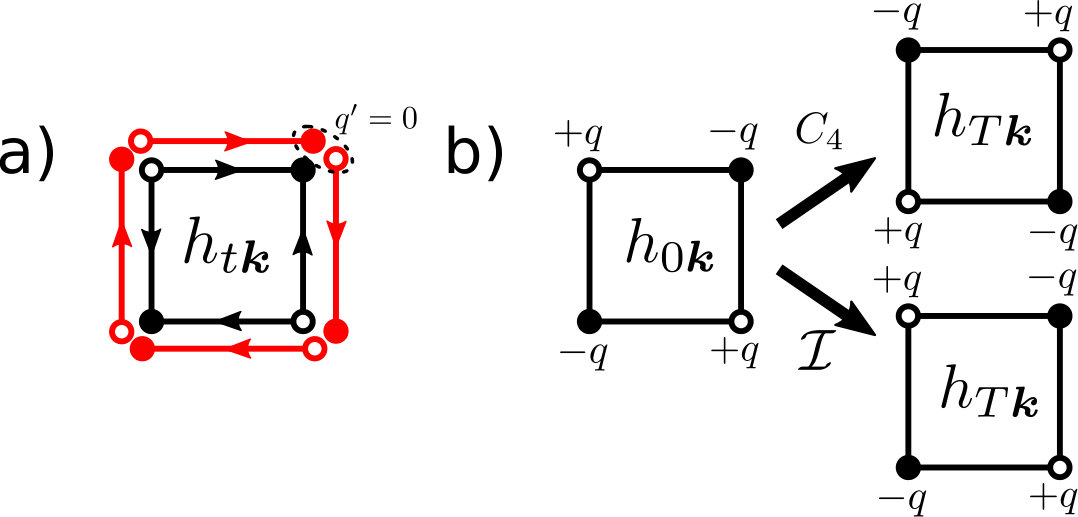 Figure 1
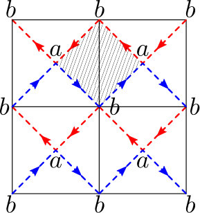 Figure 2
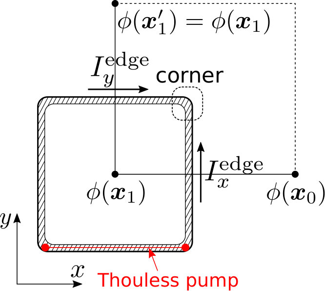 Figure 2
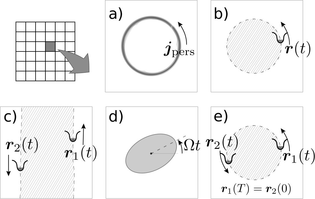 Figure 4
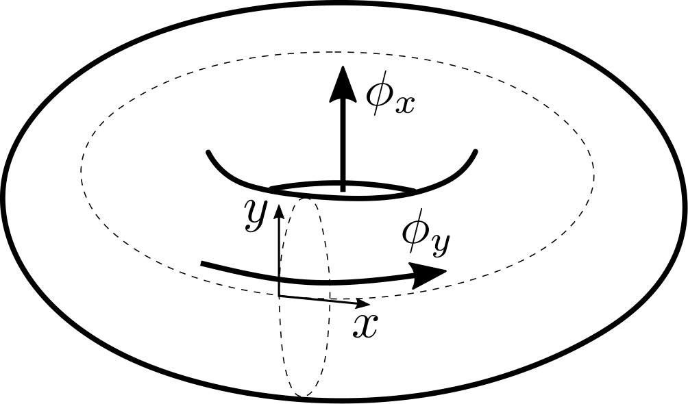 Figure 5
Peer Reviews
No public reviews on file for this paper yet. If you reviewed it on a platform where reviews are public (OpenReview, ICLR, NeurIPS, ICML), you can paste yours below so the community can read it here.
Videos
No videos yet. Explain this paper in a talk, walkthrough, or lecture? Add one.
\WarningFilter
revtex4-1Repair the float
Geometric orbital magnetization in adiabatic processes
Luka Trifunovic
RIKEN Center for Emergent Matter Science, Wako, Saitama 351-0198, Japan
Seishiro Ono
Institute for Solid State Physics, University of Tokyo, Kashiwa 277-8581, Japan
Haruki Watanabe
Department of Applied Physics, University of Tokyo, Tokyo 113-8656, Japan
Abstract
We consider periodic adiabatic processes of gapped many-body spinless electrons. We find an additional contribution to the orbital magnetization due to the adiabatic time evolution, dubbed geometric orbital magnetization, which can be expressed as derivative of the many-body Berry phase with respect to an external magnetic field. For two-dimensional band insulators, we show that the geometric orbital magnetization generally consists of two pieces, the topological piece that is expressed as third Chern-Simons form in space, and the non-topological piece that depends on Bloch states and energies of both occupied and unoccupied bands.
I Introduction
We consider periodic adiabatic processes of spinless short-range entangled phases with period at zero temperature. The ultimate goal when attacking this type of time-dependent problems on the general ground would be to obtain an expression for the physical observables induced by the time evolution in terms of instantaneous eigenstates and eigenenergies of the system.
In their pioneering works, Niu and Thouless Thouless (1983); Niu and Thouless (1984) found such an expression for the current operator uniformly averaged over the entire space. In the formulation, they assumed the periodic boundary conditions with the period for and introduced the solenoidal flux as illustrated in Fig. 1. For concreteness we work in two spatial dimensions throughout this work. Then the current operator can be expressed as
[TABLE]
(For brevity we show the dependence on time , flux , and etc., in the subscript.) Further taking an average over all values of , the expectation value of the current operator induced by the adiabatic time-evolution can be expressed as the time derivative of the many-body Berry phase for varying
[TABLE]
where is the instantaneous ground state of the Hamiltonian . This expression assumes the periodicity in (see Eqs. (17), (18) below). It is not possible to further impose the periodicity in time simultaneously. Instead we have , where is the pumped charge during in one cycle.
The result (2) is formally similar to the constitutive relation for Maxwell’s equations
[TABLE]
where and are the bulk polarization and the bulk magnetization. Later it was shown King-Smith and Vanderbilt (1993); Vanderbilt and King-Smith (1993); Resta (1994); Resta and Vanderbilt (2007) that Thouless result (2) combined with constitutive relation (3) gives a useful formula for the bulk polarization — this development marked the birth of “the modern theory” of electric polarization. The bulk polarization is given by the integral of the Berry connection (the first Chern-Simons form) [see Eq. (11) for the formula for band insulators].
Alternatively, let us impose the periodicity in time instead. In this setting it is useful to integrate over time rather than the solenoidal flux. Then the Thouless result reads Niu and Thouless (1984)
[TABLE]
where is the many-body Berry phase associated with the adiabatic time-evolution. In the thermodynamic limit, is independent of Niu and Thouless (1984); Watanabe (2018) and one can set for instance. There is also a contribution from in Eqs. (2), (4) but it is negligibly small for the same reason. We find this formulation of the Thouless pump more useful because it can be generalized to wider class of physical observables as we discuss below.
The persistent current associated with a part of the orbital magnetization can also be expressed using the instantaneous eigenstates and eigenenergies of the Hamiltonian. For band insulators, it can be written as the curl of a vector (see Fig. 2a), which together with the constitutive relation (3), allows one to define the orbital magnetization . (The subscript refers to the contribution associated with the persistent current.) Alternatively, one can evaluate the change of the instantaneous ground state energy with respect to the external magnetic field. This recent development Xiao et al. (2005); Thonhauser et al. (2005); Ceresoli et al. (2006); Shi et al. (2007) goes under the name of “the modern theory” of the orbital magnetization [see Eq. (12)]. Unlike the bulk polarization, is not related to topological response.
In this work we develop a general formulation of the remaining contribution to the electric current in the constitutive relation (3) that are neither captured by the averaged current in Eqs. (2), (4) nor by the persistent current . We find that, after coarse-graining in time, this contribution can be expressed as the curl of an additional term to the orbital magnetization so that in Eq. (3) is given by
[TABLE]
Our main result is that can be obtained as a derivative of the many-body Berry phase with respect to an external magnetic field applied in direction
[TABLE]
where represents the system size and is defined by Eq. (5) upon substitution . This expression is well-defined in two-dimensional systems with the open boundary condition at least in one direction. There are known subtleties when applying uniform magnetic field to periodic systems. See Sec. III.1 for the detailed discussion. In the following we assume vanishing Chern numbers in , and spaces.
As comparison, in the presence of an external uniform magnetic field , the instantaneous orbital magnetization gives an energy shift of the many-body ground state. (Throughout this work we set .) Accordingly, after the period , the ground state acquires an additional phase proportional . On the other hand, a non-zero value of shows up as Berry phase acquired by the many-body ground state. For this reason, we name geometric orbital magnetization. The bulk quantity is independent of the period and is defined “mod ”. This ambiguity is reflecting the possibility of decorating the boundary by one-dimensional Thouless pump.
For band insulators, we perform the perturbation theory with respect to the applied magnetic field following Refs. Shi et al., 2007; Essin et al., 2010 and find that geometric orbital magnetization consists of two contributions
[TABLE]
the topological contribution is expressed as integral of the third Chern-Simons form in space [see Eq. (51)], while the non-topological contribution is written in terms of instantaneous Bloch states and energies [Eq. (52)]. The obtained expression for of band insulators has a formal similarity with the expression for the magnetoelectric polarizability of three-dimensional band insulators Essin et al. (2010); Malashevich et al. (2010); Chen and Lee (2011) upon identification . It is worth mentioning that due to relatively large gap (order of electronvolts) of band insulators, the adiabaticity conditions is not particularly restrictive, the period can be as small as several femtoseconds.
To gain intuitive understanding of the two contributions (8), one can think of the topological piece to be originating from the Aharanov-Bohm contribution to the many-body Berry phase in the magnetic field. Thus describes the magnetization from electrons, whose positions are moving during the adiabatic process, as depicted with dashed lines and arrows in Fig. 2b-c and e. Although Fig. 2a may look similar, in Fig. 2a represents a static persistent current that is uniformly distributed on the ring. In contrast, the current density in Fig. 2b at each time is localized to the position of the potential well and it becomes divergence-free only after averaging over the period . Similarly, the non-topological piece can be understood to be originating from “spinning” of anisotropic crystalline potentials, see Fig 2d.
Let us mention at this point several related works. Adiabatic dynamics can be induced by time-dependent lattice deformations (phonons), which is the subject of studies on dynamical deformations of crystals. Ceresoli and Tosatti (2002); Juraschek et al. (2017); Juraschek and Spaldin (2018); Dong and Niu (2018); Stengel and Vanderbilt (2018) In Refs. Juraschek et al., 2017; Juraschek and Spaldin, 2018 it was shown that a time-varying polarization gives rise to a contribution to the orbital magnetization, and the semi-classical description developed in Ref. Dong and Niu, 2018 found the same effect within their framework. The time-varying polarizations in these works correspond to the situation depicted in Fig. 2b. In the case of band insulators, we find that they are captured by the abelian third Chern-Simons form. Furthermore, Refs. Ceresoli and Tosatti, 2002; Stengel and Vanderbilt, 2018 showed that rotation of molecules, as in Fig. 2d, gives rise to an orbital magnetization contribution that can be captured by relation (7). The present approach gives unified description of the above-mentioned effects. More importantly, it properly describes the orbital magnetization in adiabatic processes that have not been previously considered: the process in Fig. 2e has inversion symmetry at all times, thus polarization is time-independent, yet it gives rise to non-zero , which for the case of band insulators is captured by non-abelian third Chern-Simons form, see Sec. IV.3.
Analogous to the bulk polarization, crystalline symmetries can quantize topological geometric orbital magnetization . We show that, under certain crystalline symmetries, is related to recently discussed higher-order topological phases. Parameswaran and Wan (2017); Schindler et al. (2018); Peng et al. (2017); Langbehn et al. (2017); Song et al. (2017); Fang and Fu (2017); Ezawa (2018); Shapourian et al. (2018); Zhu (2018); Yan et al. (2018); Wang et al. (2018a, b); Khalaf et al. (2018); Khalaf (2018); Trifunovic and Brouwer (2019); Okuma et al. (2018) Among them, the topological insulators that exhibit quantized corner charges in the presence of certain crystalline symmetries attracted recently a lot of theoretical Benalcazar et al. (2017, 2017, 2019) and experimental Serra-Garcia et al. (2018); Peterson et al. (2018) attention. Although, due to crystalline symmetries, the bulk quadrupole moment is well defined in these systems (see Fig. 4a), it is still disputed in the literature whether such definition is possible in the absence of any quantizing crystalline symmetries. Kang et al. (2018); Lapa and Hughes (2018); Ono et al. (2019) Recent work in Ref. van Miert and Ortix, 2018a revealed a connection between higher-order topological insulators Parameswaran and Wan (2017); Schindler et al. (2018); Peng et al. (2017); Langbehn et al. (2017); Song et al. (2017); Fang and Fu (2017); Ezawa (2018); Shapourian et al. (2018); Zhu (2018); Yan et al. (2018); Wang et al. (2018a, b); Khalaf et al. (2018); Khalaf (2018); Trifunovic and Brouwer (2019); Okuma et al. (2018) protected by roto-inversion symmetries and adiabatic processes that involve topological insulators with quantized corner charges. In Sec. III.5 we show that the adiabatic processes discussed by van Miert and Ortix van Miert and Ortix (2018a) are characterized by quantized geometric orbital magnetization, and we relate the value of to the quantized corner charge.
The remaining of this article is organized as follows: in Sec. II we review the modern theory of the polarization and the orbital magnetization, Sec. III contains derivation of our main results, Sec. III.5 discusses the role of symmetries in the adiabatic process, and Sec. IV presents various non-interacting examples that illustrate difference between instantaneous orbital magnetization, topological and non-topological geometric orbital magnetization. More precisely, we consider toy models illustrating systems depicted in Fig. 2. As a more realistic application of physics considered in this work, we present in Sec. IV.5 calculation of magnetization induced by rotation of an insulator. A long time ago, Barnett (1915, 1935) Barnett considered magnetization of an uncharged paramagnetic material when spun on its axis. Modeling paramagnetic material as collection of local magnetic moments that are randomly oriented, Barnett Barnett (1915) argued that rotation creates a torque that acts to align local magnetic moments with rotation axis. This torque gives rise to magnetization , where is paramagnetic susceptibility, is rotation frequency and is electron gyromagnetic ratio. Barnett’s measurement of this effect Barnett (1915) provided first accurate measurement of electron gyromagnetic ratio. We calculate for this model, which, as seen from Eq. (7), is also proportional to rotational frequency and estimate quantum correction to Barnett effect. Electron contribution to has both topological and non-topological piece, but since the system is uncharged, we find that electron contribution to is canceled by corresponding ionic contribution. Thus resulting is solely due to anisotropy of crystalline potential, analogous to toy model in Fig. 2d. In Sec. V we consider examples of general interacting systems where periodic adiabatic process consists of “spinning” Ceresoli and Tosatti (2002); Stengel and Vanderbilt (2018) or “shaking” Juraschek et al. (2017); Juraschek and Spaldin (2018); Dong and Niu (2018) of the whole system. Goldman et al. (2014) Our conclusions and outlook can be found in Sec. VI.
II Preliminaries
Here we review the formulation of the polarization and the orbital magnetization for band insulators in dimensions developed in Refs. King-Smith and Vanderbilt, 1993; Vanderbilt and King-Smith, 1993; Resta, 1994; Resta and Vanderbilt, 2007; Xiao et al., 2005; Thonhauser et al., 2005; Ceresoli et al., 2006; Shi et al., 2007. To simplify notations, we assume primitive lattice vectors of the square lattice type, but this general framework is not restricted to this special choice.
II.1 Modern theory
Let us denote by the instantaneous Bloch function of -th occupied band, satisfying . Here is the single-particle Hamiltonian with a periodic potential, is the system size and is the lattice constant. We choose the cell-periodic gauge so that they obey the following conditions for any lattice vector and reciprocal lattice vector Vanderbilt (2018)
[TABLE]
According to the modern theory, the bulk polarization density is given by
[TABLE]
where is the electric charge. The sum over can be replaced with the integral over the first Brillouin zone. Similarly, the orbital magnetization density is given by
[TABLE]
where . The ambiguity in Eq. (11) can be seen by a smooth gauge transformation that changes the integral in Eq. (11) by an integer multiple of , while the integral in (12) remains unchanged.
In addition to the derivation via the Thouless pump as we described in the introduction, the formula (11) was also verified in terms of the Wannier state localized around the unit cell .
[TABLE]
In terms of the Wannier function, is the deviation of the Wannier center from , i.e., .
When the origin of unit cell is changed by , we find
[TABLE]
Namely, depends on the specific choice of the origin, while does not. Therefore, it is not itself but rather the change that is of physical interest. It also follows that for an periodic adiabatic process, where the system is translated by certain number of unit cells during the period , the orbital magnetization is periodic in time while the polarization is not.
For interacting systems under the periodic boundary condition, the combination in the parenthesis in Eq. (2) replaces Eq. (11). The periodicity in in this formulation is encoded in the relation
[TABLE]
where is the polarization operator (see Ref. Watanabe and Oshikawa, 2018 for example).
II.2 Topological response
To discuss the physical consequence of , let us recall first the topological linear response in dimension Thouless (1983) that holds at a mesoscopic scale after coarse-graining
[TABLE]
Here, () represents , and corresponds to . is a (finite dimensional) matrix constructed by occpied Bloch states and the trace in Eq. (20) is the matrix trace. Comparing with above equations, we see that is the 1D version of in Eq. (11). This response is derived starting from the Chern-Simons theory in dimensions that describes the response toward an external field and reducing the dimension to dimensions.
The parameter in Eq. (19) is a slowly varying field interpolating between two different systems. For example, an adiabatic time evolution induces the bulk current . The bulk charge transfer from to is thus given by . Similarly, a transition of one 1D system to another can be described by , giving rise to a charge density . Therefore, the total charge accumulated to the boundary is . For a given that specifies as a continuous function of and , even the integer part of is well-defined. However, only the fractional part of is independent of the detailed choice of the interpolation — the fractional part depends only on the initial and the final values of that can be individually computed by Eq. (20). What we described here can be straightforwardly translated to 2D systems. The pumped charge through the bulk per unit length along is given by , where
[TABLE]
The analog of Eq. (19) in dimensions reads Qi et al. (2008)
[TABLE]
Here, . Again, is defined by occupied Bloch states. This response is derived from the Chern-Simons theory in dimensions by a dimensional reduction. This topological response implies, for example, the magnetoelectric effect Qi et al. (2008); Essin et al. (2009, 2010) .
III Geometric orbital magnetization
In this section we present the derivations of our main results. We start with verifying the most general expression (7) for the geometric orbital magnetization. Then we derive the formula for the topological and non-topological contributions in Eq. (8).
III.1 Berry phases in adiabatic process
Suppose we are interested in the expectation value of the quantity , given by
[TABLE]
for some parameter in the Hamiltonian. For example, in the case of the averaged current operator, can be identified with the solenoidal flux [see Eq. (1)]. Likewise, for the orbital magnetization we use the external magnetic field .
Now suppose that the Hamiltonian has a periodic adiabatic dependence on , and let be the instantaneous ground state with the energy eigenvalue . We assume an excitation gap and the time-dependence of the Hamiltonian must be slow enough so that . Using the density matrix obeying the time-dependent Schrödinger equation , we express the time-average of the expectation value of as
[TABLE]
In the absence of the time-evolution, the density matrix is identical to . It acquires contributions from excited states due to the time evolution. To the lowest-order perturbation theory with respect to , the relevant matrix elements are given by Thouless (1983); Watanabe and Oshikawa (2018)
[TABLE]
Now we plug and make use of the Sternheimer identity
[TABLE]
which follows by differentiating with respect to at . In our notation, and . Combining these equations, we find
[TABLE]
where
[TABLE]
is the Berry curvature in space. Further assuming the periodicity in time
[TABLE]
we arrive at our general expression
[TABLE]
where is the time average of the expectation value using the instantaneous ground state and is the geometric contribution originating from the adiabatic time dependence. This is the generalization of Eq. (4) for the electric current to physical observables written as the derivative of Hamiltonian as in Eq. (26). The following basis-independent expressions may also be useful
[TABLE]
where is the projector onto the many-body ground state, is the many-body Green function, and the integration contour encloses only the ground state at .
Let us now specialize to the case . Then in Eq. (35) gives the geometric orbital magnetization in Eq. (7), while is the persistent current contribution. Note the additional minus sign because of . Previously, Refs. Ceresoli and Tosatti, 2002; Stengel and Vanderbilt, 2018 considered the Berry curvature in space to describe orbital magnetization induced by rotation of molecules. See also examples in Sec. IV.4 and V.1 below.
When applying these formulae, one has to be careful about boundary conditions. If open boundary conditions in at least one direction are imposed, the result (36) is directly applicable. However, a process that is periodic in time under periodic boundary condition may loose its periodicity in time under open boundary conditions. For example, the system in Fig. 2c is not periodic in time if the open boundary condition in direction is imposed. Similarly, the periodicity in time requires periodic boundary conditions in both directions for the -symmetric system in Fig. 5. Keeping (original) periodic boundary conditions in both directions in the presence of magnetic field, implies that the net flux through the system has to vanish. If the system is homogeneous, local contributions to cancel out and we cannot obtain a useful information about the system. (For single-particle problems there is a resolution as we discuss below.) Finally, one can impose magnetic periodic boundary conditions assuming that the total magnetic flux applied to the system is an integer multiple of . Brown (1964); Zak (1964) However, each eigenstate of may not be analytic as a function of despite the fact that the magnetic field itself can be made small for a large systems. The expression (36) is still applicable if the projector onto the instantaneous ground state is analytic function of , which is the case for band insulators with vanishing Chern number. Essin et al. (2010); Malashevich et al. (2010); Gonze and Zwanziger (2011); Chen and Lee (2011) However, to our knowledge there is no general proof for gapped interacting systems.
III.2 Noninteracting systems
Let us apply this general expression to noninteracting electrons described by the quadratic Hamiltonian
[TABLE]
We label single-particle states in such a way that for all . We also assume a finite gap between -th and -th levels. We write the single particle state . Then the -particle ground state can be written as
[TABLE]
For a later purpose, we allow for a unitary transformation among the occupied levels
[TABLE]
Although such a basis change may sound unnecessary, in the actual application of this framework it is sometimes important to work in the proper basis by choosing appropriately. (See Sec. III.3 for an example). After all we find that the many-body Berry phase is given by the sum of single-particle Berry phases of occupied levels
[TABLE]
Therefore, we get the following expressions for single-particle problems. The latter two expressions are basis-independent
[TABLE]
where is the projector onto occupied single-particle states, is the single-particle Hamiltonian, is single-particle Green function, and the integration contour encloses all the occupied states at ().
For the orbital magnetization, we again set . The same remarks as in the previous section apply here. In the case of band insulators, one may want to impose periodic boundary conditions to preserve the translation symmetry. As discussed in the previous section there are two possibilities to achieve this. One can change the the boundary condition to magnetic periodic boundary conditions. Brown (1964); Zak (1964) For single-particle systems, assuming symmetric gauge , the magnetic periodic boundary conditions can be taken into account explicitly by restricting the form of the projector to Essin et al. (2010); Gonze and Zwanziger (2011) , where is an arbitrary matrix function (not necessarily projector) that satisfies , where is an element of Bravais lattice. The expression for can be found perturbatively in , Essin et al. (2010); Gonze and Zwanziger (2011) which, after substituting back to Eq. (41), yields an expression for the Berry phase and . The second option is to apply a spatially modulating magnetic field as we discuss below.
III.3 Geometric orbital magnetization for band insulators
Below we consider band insulators and show that geometric orbital magnetization has two contributions as in Eq. (8). Since we assume the periodic boundary condition both in and , we apply a slowly modulating magnetic field Shi et al. (2007); Essin et al. (2010) in order to avoid changing of the boundary condition as discussed in the previous subsection. We use the vector potential
[TABLE]
with , , and . (To simplify the notation, we assume in this subsection). Such a magnetic field induces the change of the Bloch function
[TABLE]
and is given via Eq. (13).
We compute the Berry phase using the formula (41) derived above. It is important to work in the Wannier basis for which the magnetic field effectively becomes uniform in the limit . The single-particle Berry phase in this basis, summed over occupied bands, takes the following form
[TABLE]
If we further sum over , or equivalently if we work in the Bloch basis , we get [math] reflecting the fact that for bulk systems Fourier component vanishes for . Thus, care must be taken to correctly read off local contribution to — an unintentional integration over of a term proportional to makes it impossible to find the correct value of . The rest calculation follows the appendix in Ref. Essin et al., 2010. Upon taking the limit , we find
[TABLE]
This last expression can precisely be expressed as the sum of two terms, . The topological piece reads
[TABLE]
The Berry connection is defined using occupied Bloch states as a function of . The smoothness and the periodicity of are assumed in the integral in Eq. (51). Such a choice is possible only when both the pumped charge through the bulk in Eq. (22) and the 2D Chern number for vanish.
The non-topological contribution depends also on instantaneous eigenenergies of the Bloch Hamiltonian
[TABLE]
Here, is Bloch Hamiltonian, is the projector onto occupied bands at , is Bloch’s Green function, the curly brackets denote symmetrization , and the integration contour encloses all the filled Bloch states at . See the appendix of Ref. Essin et al., 2010 for the details. Note that both and are not affected by the shift of the origin in Eq. (14).
III.4 Topological contribution from response theory
Here we give an alternative, easier derivation of in Eq. (50) from the topological response theory. To this end let us further reduce one spatial dimension in Eq. (23) to achieve the topological quadratic response in d Qi et al. (2008):
[TABLE]
where is the Berry curvature in the space and and are two slowly varying fields: denotes an adiabatic and periodic time dependence and describes a smooth interface of domains (Fig. 3). In this setting, we find
[TABLE]
so that
[TABLE]
This reproduces Eq. (50). In the derivation we used the relation . It is important to note that itself cannot be written as a curl of a vector field — Eq. (III.4) holds only after the time convolution (or equivalently the time average).
The above derivation relies on the connection (3) between and topological edge current in adiabatically driven two-dimensional systems. To see this more concretely, let us consider the boundary of two regions with and (see Fig. 3). Just like in the case of polarization, only the fractional part of the edge current is the bulk contribution that depends only on and . This can be understood by noticing that decorating the boundary with a 1D chain leads to an integer charge transfer through the Thouless pump. Thouless (1983) To capture the fractional bulk contribution to the edge current, one can separately compute and without paying attention to their continuity. The geometric contribution to the charge transfer along direction, between two bulk systems with and (Fig. 3) is given by
[TABLE]
Notice that of two adjacent edges may differ by an integer. To see this formally, let us consider a charge flow into a corner surrounded by a closed curve with (see Fig. 3). The net charge flow in the process is given by the second Chern number
[TABLE]
For example, when the corner is formed by two edges along and directions, we have
[TABLE]
meaning that the charge transfer along two intersecting edges can only differ by an integer multiple of . Clearly, is not a bulk topological invariant in general, since its value can be changed by closing the boundary gap, i.e., attaching 1D Thouless pump at certain boundaries (Figs. 3 and 4b).
III.5 Symmetry constraints and corner charge
Here we consider adiabatic process of two-dimensional systems constrained by certain symmetries that quantize . We show that, if the symmetry allows one to define the bulk contribution to quadrupole moment, the quantized quadrupole moment is equal to . Such adiabatic processes were recently discussed by van Miert and Ortix, who found the connection between the quantized corner charge and higher-order topological invariant. van Miert and Ortix (2018b)
For concreteness, let us consider the four-fold rotation mapping to . It is easy to see that boundary decorations by polarized one-dimensional chains do not affect the fractional part of the corner charge , see Fig. 4a. We consider an arbitrary interpolation between the system of interest and the reference system that has no corner charge. The second half of the cycle is performed in a -symmetric manner
[TABLE]
The symmetry defined above behaves as the roto-inversion in -space, resulting in the following transformation law for :
[TABLE]
This does not mean that vanishes since it is defined only . Thus in the presence of symmetry is quantized either [math] or . When , the circulating edge current as in Fig. 3 violates symmetry constraint (60)—the only allowed edge current distribution is shown by black arrows in Fig. 4b. Note that the inversion symmetry, for example, also quantizes but the total corner charge accumulation during inversion-symmetric cycles need to vanish since the charge distribution of quadrupole moment is invariant under the inversion (see Fig. 4c).
Now we show that the parity of the corner charge accumulation is actually a bulk topological invariant for symmetric adiabatic processes satisfying constraint (60), see also Fig. 4b. To this end, consider two perpendicular edges along and direction, related to each other by symmetry. The relations (59) and (61) suggest that and that
[TABLE]
Furthermore, Fig. 4c tells us that the corner charge accumulation during the symmetric process is . Therefore,
[TABLE]
We will discuss an example of quadrupole insulators with in Sec. IV.3 using this result. On the other hand, a -symmetric phase that hosts a corner charge of were recently reported. Benalcazar et al. (2019) The fact that forces us to conclude that -symmetric adiabatic process cannot be constructed for such a phase.
Alternatively, as discussed in detail in Ref. van Miert and Ortix, 2018b, the -symmetric adiabatic process considered above, can be viewed as a 3D topological insulator protected by the roto-inversion symmetry upon identification . In fact, the 3D topological insulator with obtained this way is a second-order topological insulator. If we consider a geometry with the open boundary conditions in -plane and the periodic boundary conditions in -direction, such a second-order phase can be translationally invariant in -direction both in the bulk and on the boundary. The boundary hosts an odd number of chiral modes running along each of four hinges in -symmetric manner. Going back to the picture of an adiabatic process, it becomes clear that the corner charge accumulation is an odd integer as is varied from [math] to , which is consistent with the above result (62).
IV Examples: noninteracting systems
In this section, we discuss a simple model of noninteracting spinless electrons in a periodic potential, which highlights the distinction of two contributions to the bulk orbital magnetization, and . Additionally, we want to consider examples where there is only topological geometric magnetization, Sec. IV.3, only non-topological geometric magnetization, Sec. IV.4, and both topological and non-topological contributions, Sec. IV.5. To keep the discussions simple while capturing the relevant physics, we focus on isolated orbitals without any overlap between them.
IV.1 Bloch functions in the localized limit
Let us consider a time-dependent deep potential centering at that accommodates at least one bound state. Let be the wavefunction of the instantaneous lowest-energy bound state, satisfying with
[TABLE]
Here describes an external field. In these expressions, the superscript [math] implies the quantities for an isolated orbit. When the potential is deep enough, should be well-localized around with the localization length . Hence, we assume that
[TABLE]
and that both and decays fast enough, i.e., as .
With these building blocks, we construct a periodic potential and the cell-periodic Bloch state.
[TABLE]
We assume that respects the periodicity, i.e., . Then, as far as and () are entirely neglected, is an eigenstate of the periodic Hamiltonian
[TABLE]
with a completely flat band dispersion .
IV.2 Polarization and instantaneous magnetization
Let us first demonstrate the modern theory formula for the polarization and the orbital magnetization by deriving and in two different ways.
First, we present direct calculation of the polarization and the orbital magnetization from the microscopic charge distribution and the persistent current densities in this insulator. The instantaneous contribution to the local charge and current distribution from a single orbit can be written as
[TABLE]
We introduce vector fields and such that
[TABLE]
The existence of such is guaranteed by the divergence-free nature of the instantaneous current density . The current density induced by the adiabatic motion of is captured by in Eq. (81) whose divergence may not vanish. We assume both and decay rapidly for , which specifies the boundary condition for differential equations (71).
Physical quantities of the insulator composed of periodically arranged localized orbits can be written as the sum of the contributions from each orbit. For example microscopic current is given by
[TABLE]
and analogously for , , and . These microscopic expressions have a strong spatial dependence, periodically oscillating at the scale of . To derive to a smooth mesoscopic description, we need to perform a convolution in space (Sec. 6.6 of Ref. Jackson, 1999). Here we choose the Gaussian ()
[TABLE]
We do the same for other quantities. Relations such as are preserved by the convolution. Because the convolution is identical to the average for the periodic distribution, we find , ,
[TABLE]
This is the part of the orbital magnetization produced by the persistent current as illustrated in Fig. 2a.
Let us check that we get the same results using the general formulae of the modern theory. Because of the non-overlapping assumption of , it can be readily shown that the formula in Eqs. (11), (12) for the Bloch function (67) can be simplified to
[TABLE]
where we used Eqs. (69) and (70). These are well-known expressions in classical electrodynamics for the charge and current distributions in a confined region (see Sec. 4.1 and 5.6 of Ref. Jackson, 1999). The equivalence of Eqs. (74), (75) and (76), (77) can be easily checked by using the definition of and in Eq. (71) and integrating by parts. The second equality of Eq. (76) follows from Eqs. (65), (69), and (76).
IV.3 Topological geometric magnetization
Next, we discuss the topological geometric contribution for this model. To this end, suppose that the position of the potential minimum adiabatically moves as a function of and forms a closed curve as illustrated in Fig. 2b. We assume the form of the potential, and thus the localization length, remains unchanged during the adiabatic process.
We first apply our general expression for in Eq. (50) to the Bloch function (67). Thanks to the non-overlapping assumption, the vector potential is -independent:
[TABLE]
with . Plugging this into Eq. (51), we find
[TABLE]
where represents the area enclosed by the orbit of in one cycle. Therefore,
[TABLE]
Observe the analogy to in Eq. (77). This expression does not have integer ambiguity because it is given by abelian third Chern-Simons form.
Let us verify this result from a direct calculation. The adiabatic motion of the single orbit following the potential minimum at induces a local current distribution
[TABLE]
It becomes divergence-free if averaged over one period
[TABLE]
As we have seen above, the sum of such microscopic currents from each unit cell produces the bulk magnetization
[TABLE]
This agrees with Eq. (80) because the integral in the parenthesis is precisely due to Eq. (65).
The result in Eq. (80) can be readily generalized to the case with multi-orbitals, such as examples in Fig. 2c and e. Let us introduce potential minima () in each unit cell, which are adiabatically varied as a function of . This time, each orbit is allowed to form an open curve, as far as the total polarization satisfies . Under such an assumption, we find that
[TABLE]
We present the proof in the Appendix A. Although the above expression appears to be the sum of single-band contributions, the “would-be” contribution from each band depends on the specific choice of the origin when it does not form a closed loop. Only after performing the summation over all occupied bands, or in other words, only after fully taking into account the non-abelian nature of the third Chern-Simons form, the result restores the independence from the origin choice.
As the application of the formula (85), let us discuss the corner charge of the -symmetric quadrupole insulator introduced in Refs. Benalcazar et al., 2017, 2017. For the wallpaper group , there exist three spacial Wyckoff positions: the unit cell origin at , the center of the plaquette at , and the center of bonds at , . Hahn (2006) In the nontrivial phase, the two occupied Wannier orbitals locate at , while in the trivial phase they are at . We consider a periodic adiabatic process illustrated in Fig. 5 starting with the nontrivial phase at and passing the trivial phase at . The instantaneous Hamiltonian itself breaks the -symmetry down to symmetry except when and , while the adiabatic process as a whole implements the full in the sense of Eq. (60). We can readily compute of this process using Eq. (85) which turns out to be . This is the corner charge of the quadrupole insulator as predicted by Eq. (63), which agrees with the original study. Benalcazar et al. (2017, 2017) A variant of this adiabatic process was also discussed in Ref. van Miert and Ortix, 2018b.
IV.4 Non-topological geometric magnetization
In this example we first consider a single electron in an anisotropic and rotating two-dimensional well, Goldman et al. (2014) see Fig. 2d. We assume a harmonic confining potential, i.e., Hamiltonian (64) with
[TABLE]
where and . To obtain the geometric orbital magnetization for this model, we consider external magnetic field described by the vector potential . (Strictly speaking, this form is valid only around the origin as it lacks the required periodicity.) The wave function of the instantaneous ground state of this model can be obtained based on Ref. Rebane, 2012:
[TABLE]
where is the normalization factor and is the cyclotron frequency. The Berry phase during the adiabatic process is
[TABLE]
From Eq. (7) it follows that the adiabatic process (87) has non-zero geometric orbital magnetic moment
[TABLE]
Now we construct the Bloch function (67) using as the building block and compute the geometric orbital magnetization based on Eq. (52) for the corresponding band insulator. To this end we need instantaneous eigenstates and eigenenergies in absence of external magnetic field including unoccupied bands. The Hamiltonian is given by Eq. (68) with given by Eq. (87) and . We assume that there is no overlap between wavefunctions belonging to different unit cells as before. (When are large enough, such an assumption is valid at least for relevant low-energy states.) Bloch wavefunctions read
[TABLE]
where labels energy levels of two-dimensional the anisotropic harmonic oscillator and corresponds to the ground state in Eq. (88) with . Substituting above expressions to Eqs. (50) and (52), we find
[TABLE]
IV.5 Geometric magnetization by rotation
Here we calculate the contribution to the geometric orbital magnetization of a rotating uncharged body and compare it to the classical Barnett effect. Barnett (1915, 1935) The Barnett effect predicts magnetization , where is the paramagnetic susceptibility, is the electron gyromagnetic ratio, and is the rotation frequency. Since the rotation axis does not necessarily coincide with potential well minima we have with from Eq. (87) and , where is the distance of the potential well minima to the rotation axis. The lowest-energy instantaneous wavefunction can be obtained from Eq. (88) by performing gauge transformation
[TABLE]
As compared to Eq. (89), the Berry phase during the adiabatic process acquires an additional contribution from the Aharonov-Bohm phase. Therefore electrons contribute to the following geometric orbital magnetization
[TABLE]
The first term can be identified with in Eq. (80) and the second term is the contribution in Eq. (90). Since the body is uncharged, the contribution from ions cancels the topological contribution, while remains since ions are much more localized compared to electrons. Assuming anisotropy , and confinement of electrons on the scale of angstroms, we find that contribution (93) is on the same order as Barnett effect for paramagnets with paramagnetic susceptibility . For comparison, paramagnets have typically magnetic susceptibility . Wikipedia contributors (2019)
V Examples: finite interacting systems
In this section we demonstrate the validity of Eq. (7) for finite interacting systems. We consider two canonical ways of introducing the time-dependence to the Hamiltonian: rotating Ceresoli and Tosatti (2002); Stengel and Vanderbilt (2018) and translating the whole system. Goldman et al. (2014); Juraschek et al. (2017); Dong and Niu (2018)
We consider many-body systems under the open boundary condition in two spatial dimensions. We start with a time-independent Hamiltonian that can contain arbitrary interactions. The total charge, current, polarization, and orbital magnetization operator for this Hamiltonian can be written as , , , . We stress that these expressions are valid only when the system is confined in a finite region; they need to be modified in extended systems under the periodic boundary conditions as done by the modern theory. We denote the many-body ground state of and its energy by and , respectively.
To compute the many-body Berry phase, let be the Hamiltonian with the vector potential in the symmetric gauge with . Expanding to the linear order in and using , we get
[TABLE]
Therefore, the ground state of to the leading order in can be expressed as
[TABLE]
Here is the projector onto excited states.
V.1 Rotation
Here we consider the time-dependence of the problem induced by the rotation of the whole system
[TABLE]
where is the rotation frequency and is the angular momentum operator. For the time-dependent Hamiltonian , the orbital magnetization operator
[TABLE]
We evaluate the instantaneous contribution and the geometric contribution to the orbital magnetization via the formulae in Eqs. (34) and (35). The instantaneous contribution is given by the instantaneous ground state
[TABLE]
The geometric contribution is given by the many-body Berry phase. Since the instantaneous ground state of the Hamiltonian is given by , we have
[TABLE]
This is the expectation value of in the presence of the perturbation in Eq. (96). Using Eq. (97), we get
[TABLE]
We verify these results by solving time-dependent problem. The solution to the time-dependent Schrödinger equation can be readily constructed using the ground state of the time-independent Hamiltonian
[TABLE]
The solution that is smoothly connected to the ground state in the static limit reads
[TABLE]
The time-average of the orbital magnetization is thus given by
[TABLE]
This is the expectation value of in the presence of the perturbation as in Eq. (103). The first-order perturbation theory with respect to gives
[TABLE]
This is precisely predicted above in Eqs. (100) and (102). As it is clear from the derivation, the agreement of the two independent approaches is guaranteed by the Maxwell relation for the free energy
[TABLE]
V.2 Translation
Next let us introduce the time-dependence by the translation. All discussions proceed in essentially the same way, while there are still a few differences. First we define the time-dependent Hamiltonian by
[TABLE]
where is the translation by amount and is the momentum operator. For the orbital magnetization operator becomes
[TABLE]
where the second term in the parenthesis is due to the change of the origin. The instantaneous ground state gives as in Eq. (100), where we used .
Next, we compute the geometric contribution via the many-body Berry phase. In the presence of magnetic field translation operator becomes translation followed by gauge transformation Brown (1964); Zak (1964)
[TABLE]
The instantaneous ground state of is , thus the many-body Berry phase reads
[TABLE]
Here, represents the area swept by in one cycle. In the derivation, we used
[TABLE]
Therefore, when the whole system is translated, the geometric contribution to the orbital magnetization captures the Aharonov-Bohm phase
[TABLE]
To verify the above results, we consider the time-dependent Schrödinger equation . An approximate solution is given by , where is the instantaneous ground state of the Hamiltonian . Therefore, the time-average of the orbital magnetization is
[TABLE]
In the adiabatic limit, this reproduces in Eqs. (100) and (113). In the derivation we used for the ground state of .
VI Conclusion
In order to obtain current and charge distribution in a medium, one needs to solve Maxwell’s equation together with two constitutive relations [see Eq. (3)] that fully characterize the medium at the mesoscopic scale. The modern theories, developed in the last 30 years, provide handy formulae to calculate electric polarization King-Smith and Vanderbilt (1993); Vanderbilt and King-Smith (1993); Resta (1994); Resta and Vanderbilt (2007) and orbital magnetization Xiao et al. (2005); Thonhauser et al. (2005); Ceresoli et al. (2006); Shi et al. (2007) for realistic materials.
The focus of this work is on spinless short-range entangled systems under periodic adiabatic evolution. Our main result is to identify an additional contribution to the orbital magnetization that we name geometric orbital magnetization . This new contribution is defined only after performing the time-average over the period of the adiabatic process, which makes the current density divergence-free. We find that the geometric orbital magnetization can be expressed compactly as derivative of the many-body Berry phase with respect to an externally applied magnetic field. For band insulators, we obtain handy formulae for the bulk geometric orbital magnetization in terms of instantaneous Bloch states and energies. Interestingly, we find that for band insulators consists of two pieces, where topological piece depends only on the Bloch states of occupied bands. For spinless systems only electric polarization and orbital magnetization enter constitutive relations, since the contributions from higher moments are typically negligible. Jackson (1999) In this sense, our results together with “the modern theories” provide a complete mesoscopic description of a medium under periodic adiabatic time evolution. In this work we have not considered adiabatic processes with ground state degeneracy, Meidan et al. (2011) it would be interesting to see to which extent our findings can be generalized to such systems.
In the present work, the adiabaticity assumption is crucial for validity of the obtained results. In practice, for band insulators with band gaps on the order of electronvolt, this conditions requires that the period is larger than couple of femtoseconds. Nevertheless, shorter period results in a larger geometric orbital magnetization. It would be therefore interesting to extend our results to the case of strong drive that excites unoccupied bands. In the case of Thouless pumps such extension was very fruitful and resulted in recent discovery of shift currents. von Baltz and Kraut (1981); Morimoto and Nagaosa (2016)
Although higher (than dipole) electric and magnetic multiple moments typically do not enter constitutive relations, the knowledge of these quantities may be useful for certain systems. Benalcazar et al. (2017, 2019) In fact, it is a topic of current research whether higher moments can be established as bulk quantities in general. Gao and Xiao (2018); Shitade et al. (2018); Kang et al. (2018); Lapa and Hughes (2018); Ono et al. (2019) In the presence of certain crystalline symmetries, both electric polarization and topological geometric orbital magnetization can be quantized, in which case they can serve as a topological invariants. In this context, we showed that the quantized quadrupole moment is related to in systems with proper symmetries that allow bulk definition of the quadrupole moment. Ono et al. (2019)
In this work we succeeded in separating into the topological and the non-topological piece only for band insulators. There, we found that the topological contribution is expressed as the third Chern-Simons form (), in space. For interacting systems, based on examples considered in Sec. V, we conclude that it is possible to separate Aharonov-Bohm contribution originating from the center of mass motion. In fact, this contribution can be captured by calculating formally defined for the many-body ground state as a function of time and two solenoidal fluxes. Clearly, the many-body defined in such manner is abelian and does not capture all possible topological contributions. For example, it vanishes for the model in Fig. 4. As a future direction, it would be interesting to see if separation achieved for band insulators is possible for general single-particle, or even many-body systems. The affirmative answer to this question would provide a way to define in two dimensional systems with adiabatic time-dependence lacking the translational invariance or the single-particle description. The formula for in many-body three-dimensional systems already exist in the literature, Wang and Zhang (2014); Shiozaki et al. (2018) where it was argued that is related to the magnetoelectric polarizability. The magnetoelectric polarizability of three-dimensional materials contains, at least for the case of band insulators, not only topological but also non-topological contribution, Essin et al. (2010) thus the analogous “separation question” arises also in that context. Additionally, defining quantized quadrupole moment for interacting systems is one of the open questions. Kang et al. (2018); Lapa and Hughes (2018); Ono et al. (2019) Since for band insulators we find connection between and quantized quadrupole moment, separating contribution in interacting systems might provide useful many-body definition of quantized quadrupole moment.
We hope that our work will also have practical implication as it contributes to emerging field of “dynamical material design” by providing a way to calculate additional orbital magnetization contribution that appears in these systems. Ceresoli and Tosatti (2002); Juraschek et al. (2017); Juraschek and Spaldin (2018); Dong and Niu (2018); Stengel and Vanderbilt (2018)
Acknowledgements.
We would like to thank David Vanderbilt for drawing Refs. Ceresoli and Tosatti, 2002; Juraschek et al., 2017; Juraschek and Spaldin, 2018; Dong and Niu, 2018; Stengel and Vanderbilt, 2018 to our attention. The work of S.O. is supported by Materials Education program for the future leaders in Research, Industry, and Technology (MERIT). The work of H.W. is supported by JSPS KAKENHI Grant No. JP17K17678 and by JST PRESTO Grant No. JPMJPR18LA.
Appendix A Topological geometric orbital magnetization in simple models
Here we present the derivation of Eq. (85) in Sec. IV.3 for multi potential minima at (). To calculate the geometric orbital magnetization, we use the cell-periodic Bloch state (67) for each orbital. Substitution of with [c.f. Eq. (78)] into Eq. (51), we find
[TABLE]
However, this is not the complete expression of because Eq. (78) implies that the above Berry connection violates the periodicity in time when differs from . To quantify the violation, let us introduce the mismatch matrix
[TABLE]
To repair periodicity of we need to find a family of unitary matrices that interpolates and . Such an interpolation exists if and only if the polarization satisfy . Accordingly, below we focus on the case . The gauge transformation with this gives a periodic Berry connection
[TABLE]
as far as
[TABLE]
The full expression of is given by computing Eq. (51) with . It is given by Ryu et al. (2007)
[TABLE]
where the sum over and are assumed. is the Pontryagin index of the matrix , which requires an explicit expression for , whereas the knowledge of mismatch matrix in Eq. (116) suffices for the boundary term . It reads
[TABLE]
Thus, in order to prove (85), it remains to show that . Below we show this by explicitly constructing .
Consider a family of unitary matrices
[TABLE]
with and . The above matrix interpolates between unitary matrix and the identity matrix . We also require so that the requirement (118) is satisfied. One such function is given by
[TABLE]
Since depends only on , it is easy to check that its Pontryagin index vanishes. We then define by a composition
[TABLE]
where each interpolation matrix is defined as,
[TABLE]
with
[TABLE]
It is straightforward to check that equals to the identity matrix and that the Pontryagin index for each vanishes.
The reference list from the paper itself. Each links out to its DOI / PubMed record.
- 1Thouless (1983) D. J. Thouless, Phys. Rev. B 27 , 6083 (1983) . · doi ↗
- 2Niu and Thouless (1984) Q. Niu and D. J. Thouless, Journal of Physics A: Mathematical and General 17 , 2453 (1984) . · doi ↗
- 3King-Smith and Vanderbilt (1993) R. D. King-Smith and D. Vanderbilt, Phys. Rev. B 47 , 1651 (1993) . · doi ↗
- 4Vanderbilt and King-Smith (1993) D. Vanderbilt and R. D. King-Smith, Phys. Rev. B 48 , 4442 (1993) . · doi ↗
- 5Resta (1994) R. Resta, Rev. Mod. Phys. 66 , 899 (1994) . · doi ↗
- 6Resta and Vanderbilt (2007) R. Resta and D. Vanderbilt, Physics of Ferroelectrics: A Modern Perspective (Springer Berlin Heidelberg, Berlin, Heidelberg, 2007) pp. 31–68. · doi ↗
- 7Watanabe (2018) H. Watanabe, Phys. Rev. B 98 , 155137 (2018) . · doi ↗
- 8Xiao et al. (2005) D. Xiao, J. Shi, and Q. Niu, Phys. Rev. Lett. 95 , 137204 (2005) . · doi ↗