New integral transform: Shehu transform a generalization of Sumudu and Laplace transform for solving differential equations
Shehu Maitama, Weidong Zhao

TL;DR
This paper introduces the Shehu transform, a new integral transform generalizing Laplace and Sumudu transforms, designed to improve the solving of differential equations with increased efficiency and accuracy.
Contribution
The Shehu transform is a novel integral transform derived from Fourier transform, providing a unified approach to solve differential equations more effectively.
Findings
Successfully derived from Fourier transform
Effective in solving ordinary differential equations
High accuracy demonstrated in applications
Abstract
In this paper, we introduce a Laplace-type integral transform called the Shehu transform which is a generalization of the Laplace and the Sumudu integral transforms for solving differential equations in the time domain. The proposed integral transform is successfully derived from the classical Fourier integral transform and is applied to both ordinary and partial differential equations to show its simplicity, efficiency, and the high accuracy.
Click any figure to enlarge with its caption.
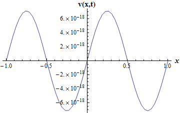 Figure 1
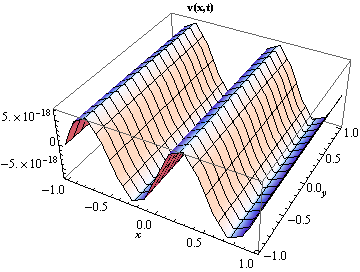 Figure 2
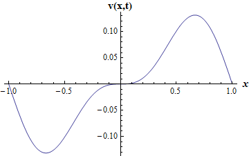 Figure 3
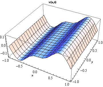 Figure 4
| S.NO. | |||||
| 1 | 1 | 1 | |||
| 2 | |||||
| 3 | |||||
| 4 | |||||
| 5 | |||||
| 6 | |||||
| 7 | |||||
| 8 | |||||
| 9 | |||||
| 10 | |||||
| 11 | |||||
| 12 | |||||
| 13 | |||||
| 14 | |||||
| 15 | |||||
| 16 | |||||
| 17 | |||||
| 18 | |||||
| 19 | |||||
| 20 | |||||
| 21 | |||||
| 22 | (Sine integral) | ||||
| 23 | (Cosine integral) | ||||
| 24 | (Exp. integral) | ||||
| 25 | |||||
| 26 | |||||
| 27 | |||||
| 28 | |||||
| 29 | |||||
| 30 | |||||
| 31 | |||||
| 32 | |||||
| 33 | |||||
| 34 | |||||
| 35 |
| S.NO. | Definition/Property | Transforms | |
| 1 | Definition | ||
| 2 | Inverse | ||
| 3 | Linearity | ||
| 4 | Change of scale | ||
| 5 | Derivatives | ||
| S.No. | Integral transform | Definition |
| 1 | Laplace transform | |
| 2 | Fourier transform | |
| 3 | Melling transform | |
| 4 | Hankel’s transform | |
| 5 | Sumudu transform | |
| 6 | Laplace-Carson transform | , |
| 7 | Atangana-Kilicman transform | |
| 8 | El-zaki transform | |
| 9 | Yang transform | |
| 10 | natural transform | |
| 11 | z-transform | |
| 12 | -transform |
Peer Reviews
No public reviews on file for this paper yet. If you reviewed it on a platform where reviews are public (OpenReview, ICLR, NeurIPS, ICML), you can paste yours below so the community can read it here.
Videos
No videos yet. Explain this paper in a talk, walkthrough, or lecture? Add one.
NEW INTEGRAL TRANSFORM: SHEHU TRANSFORM A GENERALIZATION OF SUMUDU AND LAPLACE TRANSFORM FOR SOLVING DIFFERENTIAL EQUATIONS
SHEHU MAITAMA∗, WEIDONG ZHAO**
School of Mathematics, Shandong University, Jinan, Shandong 250100, P.R. China
∗Corresponding author: [email protected]
Abstract.
In this paper, we introduce a Laplace-type integral transform called the Shehu transform which is a generalization of the Laplace and the Sumudu integral transforms for solving differential equations in the time domain. The proposed integral transform is successfully derived from the classical Fourier integral transform and is applied to both ordinary and partial differential equations to show its simplicity, efficiency, and the high accuracy.
Key words and phrases:
Shehu transform; Fourier integral transform; Laplace transform; natural transform; Sumudu transform; ordinary and partial differential equations.
2010 Mathematics Subject Classification:
44A10, 44A15, 44A20, 44A30, 44A35
1. Introduction
Historically, the origin of the integral transforms can be traced back to the work of P. S. Laplace in 1780s and Joseph Fourier in 1822. In recent years, differential and integral equations have been solved using many integral transforms ([1]-[11]). The Laplace transform, and Fourier integral transforms are the most commonly used in the literature. The Fourier integral transform [12] was named after the French mathematician Joseph Fourier. Mathematically, Fourier integral transform is defined as:
[TABLE]
The Fourier transform have many applications in physics and engineering processes [13]. The Laplace integral transform is similar with the Fourier transform and is defined as:
[TABLE]
The Laplace transform is highly efficient for solving some class of ordinary and partial differential equations [14]. By replacing the variable with the variable in Equ.(1.1), the well-known Fourier transform will become a Laplace transform and the vice-versa. The only difference between the Laplace transform, and the Fourier transform is that the Laplace transform can be defined for both stable and unstable system while the Fourier transform can only be defined on a stable system. In mathematical literature, the discrete-time equivalent of the Laplace transform called z-transform [15] converts a discrete-time signal into a complex frequency-domain representation. The basic idea of the z-transform was known to Laplace and later it was re-introduced by the Jewish-Polish mathematician Witold Hurewicz to treat a sampled-data control systems used with radar in 1947 ([16]-[17]). In mathematics and signal processing, the bilateral or two-sided z-transform of a discrete-time signal is the normal power series which is defined as:
[TABLE]
where is an integer and is in general a complex number [18].
The multiplicative version of the two-sided Laplace transform called the Mellin integral transform is defined as [19]:
[TABLE]
The Mellin integral transform is similar with the Laplace transform and Fourier transform and is widely applied in computer science and number theory due to its invariant property [20, 21]. In railway engineering, the Laplace-Carson transform [22] which is a Laplace-type integral transform named after Pierre Simon Laplace and John Renshaw Carson is defined as:
[TABLE]
The Laplace-Carson integral transform have many applications in physics and engineering and can easily be converted into a Mellin deconvolution problem, see ([23],[24]). In mathematics, the Hankel’s integral transform [25] which is similar to the Fourier transform was first introduced by the German mathematician Hermann Hankel and was widely used in physical science and engineering [26]. The Hankel’s transform is defined as:
[TABLE]
where is the Bessel function of the first kind of order with .
In 1993, Watugala introduced a Laplace-like integral transform called the Sumudu integral transform [27]. In recent years, Sumudu transform has been applied to many real-life problems because of its scale and unit preserving properties ([28]-[31]). The mathematical definition of the Sumudu transform is given by:
[TABLE]
provided the integral exists for some . Based on the basic idea of the Laplace and the Sumudu integral transform, the Elzaki transform was proposed in 2011. The Elzaki transform is closely related with the Laplace transform, Sumudu transform, and the natural transform. Elzaki transform is defined as [32]:
[TABLE]
provided the integral exists for some .
The natural transform [33] which is similar to Laplace and Sumudu integral transform was introduced in 2008. In recent years, natural transform was successfully applied to many applications (see [34, 35]). The natural transform is defined by the following integral:
[TABLE]
provided the integral exists for some variables and . Recently, a new integral transform called the -transform which is also similar to natural transform is introduced by Srivastava et al. in 2015. Mathematically speaking, -transform is closely connected with the well-known Laplace transform and the Sumudu integral transform. -transform was successfully applied to first order initial-boundary value problem (see Srivastava et al. [36]). The -transform is defined as:
[TABLE]
where both and are the -transform variables.
In 2013, Atangana and Kilicman introduced a novel integral transform called the Abdon-Kilicman integral transform [37] for solving some differential equations with some kind of singularities. The novel integral transform is defined as:
[TABLE]
The Atangana-Kilicman integral becomes Laplace transform when . Recently, a Laplace-type integral transform called the Yang transform ([38]-[40]) for solving steady heat transfer problems was introduced in 2016. The integral transform is defined as:
[TABLE]
provided the integral exists for some .
Due to the rapid development in the physical science and engineering models, there are many other integral transforms in the literature. However, most of the existing integral transforms have some limitations and cannot be used directly to solved nonlinear problems or many complex mathematical models. As a result, many authors became highly interested to come up with the alternative approach for solving many real-life problems. In 2016, Atangana and Alkaltani introduced a new double integral equation and their properties based on the Laplace transform and decomposition method. The double integral transform was successfully applied to second order partial differential equation with singularity called the two-dimensional Mboctara equation [41]. Recently, Eltayeb applied double Laplace decomposition method to nonlinear partial differential equations [42]. In 2017, Belgacem el at. extended the applications of the natural and the Sumudu transforms to fractional diffusion and Stokes fluid flow realms [43].
Motivated by the above-mentioned researches, in this paper we proposed a Laplace-type integral transform called Shehu transform for solving both ordinary and partial differential equations. The Laplace-type integral transform converges to Laplace transform when , and to Yang integral transform when . The proposed integral transform is successfully applied to both ordinary and partial differential equations. All the results obtained in the applications section can easily be verified using the Laplace or Fourier integral transforms. Throughout this paper, the Shehu transform is denoted by an operator .
2. Main result
Definition 1**.**
*The Shehu transform of the function of exponential order is defined over the set of functions,
,
by the following integral*
[TABLE]
It converges if the limit of the integral exists, and diverges if not.
The inverse Shehu transform is given by
[TABLE]
Equivalently
[TABLE]
where and are the Shehu transform variables, and is a real constant and the integral in Equ.(2.3) is taken along in the complex plane .
Theorem 1**.**
The sufficient condition for the existence of Shehu transform. If the function is piecewise continues in every finite interval and of exponential order for . Then its Shehu transform exists.
Proof. For any positive number , we algebraically deduce
[TABLE]
Since the function is piecewise continues in every finite interval , then the first integral on the right hand side exists. Besides, the second integral on the right hand side exists, since the function is of exponential order for . To verify this claim, we consider the following case
[TABLE]
The proof is complete.
Property 1**.**
Linearity property of Shehu transform. Let the functions and be in set A, then A, where and are nonzero arbitrary constants, and
[TABLE]
Proof. Using the Definition 1 of Shehu transform, we get
[TABLE]
The proof is complete.
In particular, using the Definition 1 and Property 1, we obtain
[TABLE]
[TABLE]
see entries of table 1.
Property 2**.**
Change of scale property of Shehu transform. Let the function be in set A, where is an arbitrary constant. Then
[TABLE]
Proof. Using the Definition 1 of Shehu transform, we deduce
[TABLE]
Substituting which implies and in Equ.(2.7) yields
[TABLE]
The proof is complete.
Theorem 2**.**
Derivative of Shehu transform. If the function is the derivative of the function with respect to , then its Shehu transform is defined by
[TABLE]
When n=1, 2, and 3 in Equ. (2.8) above, we obtain the following derivatives with respect to .
[TABLE]
[TABLE]
[TABLE]
Proof. Now suppose Equ. (2.8) is true for . Then using Equ. (2.9) and the induction hypothesis, we deduce
[TABLE]
which implies that Equ. (2.8) holds for . By induction hypothesis the proof is complete.
The following important properties are obtain using the Leibniz’s rule
[TABLE]
[TABLE]
and
[TABLE]
3. Some useful results of Shehu transform
Property 3**.**
Let the function be in set A. Then its Shehu transform is given by
[TABLE]
Proof. Using Equ.(2.1), we deduce
[TABLE]
This ends the proof.
Property 4**.**
Let the function be in set A. Then its Shehu transform is given by
[TABLE]
Proof. Using the Definition 1 of the Shehu transform and integration by parts, we get
[TABLE]
Thus the proof ends.
Property 5**.**
Let the function be in set A. Then its Shehu transform is given by
[TABLE]
Proof. From the Definition 1 of the Shehu transform and integration by parts, we deduce
[TABLE]
The proof is completed.
Property 6**.**
Let the function be in set A. Then its Shehu transform is given by
[TABLE]
The proof of property 6 follows immediately from the previous property 5.
Property 7**.**
Let the function be in A. Then its Shehu transform is given by
[TABLE]
Proof. Using Equ.(2.1), we get
[TABLE]
This ends the proof.
Property 8**.**
Let the function be in set A. Then its Shehu transform is given by
[TABLE]
Proof. Using the Definition 1 of the Shehu transform and integration by parts, we get
[TABLE]
The proof is complete.
Property 9**.**
Let the function be in set A. Then its Shehu transform is given by
[TABLE]
Proof. Using the Definition 1 of the Shehu transform and integration by parts, we deduce
[TABLE]
Thus the proof is complete.
Property 10**.**
Let the function be in set A. Then its Shehu transform is given by
[TABLE]
The proof of Property 10 follows as a direct consequence of Property 9.
Property 11**.**
Let the function be in set A. Then its Shehu transform is given by
[TABLE]
Proof. Using the Definition 1 of the Shehu transform and integration by parts, we get
[TABLE]
Simplifying the required integrals complete the proof of Property 11.
Property 12**.**
Let the function be in set A. Then its Shehu transform is given by
[TABLE]
Proof. Using the Definition 1 of the Shehu transform and integration by parts, we deduce
[TABLE]
Simplifying the required integrals complete the proof of Property 12.
Property 13**.**
Let the function be in set A. Then its Shehu transform is given by
[TABLE]
Proof. From the Definition 1 of the Shehu transform and integration by parts, we get
[TABLE]
Simplifying the required integrals complete the proof of Property 13.
Property 14**.**
Let the function be in set A. Then its Shehu transform is given by
[TABLE]
Proof. Applying the Definition 1 of the Shehu transform and integration by parts, we get
[TABLE]
Collecting the required integrals complete the proof of Property 14.
Property 15**.**
Let the function be in set A. Then its Shehu transform is given by
[TABLE]
Proof. Using the Definition 1 of the Shehu transform and integration by parts, we deduce
[TABLE]
Simplifying the required integrals complete the proof of property 15. This ends the proof.
Property 16**.**
Let the function be in set A. Then its Shehu transform is given by
[TABLE]
Proof. Applying the Definition 1 of the Shehu transform and integration by parts, we get
[TABLE]
Simplifying the required integrals complete the proof of property 16.
Property 17**.**
Let the function be in set A. Then its Shehu transform is given by
[TABLE]
Proof. Using the definition of Shehu transform, we get
[TABLE]
The proof is complete.
Property 18**.**
Let the function be in set A. Then its Shehu transform is given by:
[TABLE]
**Proof:
Using the definition of Shehu transform, we get**
[TABLE]
This ends the proof.
More properties of the Shehu transform and their converges to the natural transform, the Sumudu transform, and the Laplace transform are presented in table 1. The comprehensive summary of Shehu transform properties are presented in table 2.
4. Applications
In this section, the applications of the proposed transform are presented. The simplicity, efficiency and high accuracy of the Shehu transform are clearly illustrated.
Example 1**.**
Consider the following first order ordinary differential equation
[TABLE]
subject to the initial condition
[TABLE]
Applying the Shehu transform on both sides of Equ. (4.1), we get
[TABLE]
Substituting the given initial condition and simplifying, we deduce
[TABLE]
Taking the inverse Shehu transform of Equ. (4.4), yields
[TABLE]
Example 2**.**
Consider the following second order ordinary differential equation
[TABLE]
subject to the initial conditions
[TABLE]
Applying the Shehu transform on both sides of Equ. (4.6), we obtain
[TABLE]
Substituting the given initial conditions and simplifying, we deduce
[TABLE]
Taking the inverse Shehu transform of Equ. (4.9), we get
[TABLE]
Example 3**.**
Consider the following second nonhomogeneous order ordinary differential equation
[TABLE]
subject to the initial conditions
[TABLE]
Applying the Shehu transform on both sides of Equ. (4.11), yields
[TABLE]
Substituting the given initial conditions and simplifying, we obtain
[TABLE]
Taking the inverse Shehu transform of Equ. (4.14), we get
[TABLE]
Example 4**.**
Consider the following ordinary differential equation
[TABLE]
subject to the initial conditions
[TABLE]
Applying the Shehu transform on both sides of Equ. (4.16), we get
[TABLE]
Substituting the given initial conditions and simplifying, we get
[TABLE]
Taking the inverse Shehu transform of Equ. (4.19), we get
[TABLE]
Example 5**.**
Consider the following homogeneous partial differential equation
[TABLE]
subject to the boundary and initial conditions
[TABLE]
Applying the Shehu transform on both sides of Equ. (4.21), we get
[TABLE]
Substituting the given initial condition and simplifying, we get
[TABLE]
The general solution of Equ. (4.24) can be written as
[TABLE]
where is the solution of the homogeneous part which is given by
[TABLE]
and is the solution of the nonhomogeneous part which is given by
[TABLE]
Applying the boundary conditions on Equ. (4.26), we get
[TABLE]
since .
Using the method of undetermined coefficients on the nonhomogeneous part, we get
[TABLE]
Since, and .
Then Equ. (4.25) will become
[TABLE]
Taking the inverse Shehu transform of Equ. (4.29), we get
[TABLE]
Figure 1. 3D and 2D surfaces of the analytical solution of Equ. (4.21) in the ranges , and , when .
Example 6**.**
Consider the following nonhomogeneous partial differential equation
[TABLE]
subject to the boundary and initial conditions
[TABLE]
Applying the Shehu transform on both sides of Equ. (4.31), we get
[TABLE]
Substituting the given initial condition and simplifying, we get
[TABLE]
The general solution of Equ. (4.34) can be written as
[TABLE]
where is the solution of the homogeneous part which is given by
[TABLE]
and is the solution of the nonhomogeneous part which is given by
[TABLE]
Applying the boundary conditions on Equ. (4.36), we deduce
[TABLE]
since .
Using the method of undetermined coefficients on the nonhomogeneous part, we get
[TABLE]
since,
[TABLE]
Then Equ. (4.35) will becomes
[TABLE]
Taking the inverse Shehu transform of Equ. (4.39), we get
[TABLE]
Figure 2. 3D and 2D surfaces of the analytical solution of Equ. (4.31) in the ranges , and .
5. Conclusion
We introduced an efficient Laplace-type integral transform called the Shehu transform for solving both ordinary and partial differential equations. We presented its existence and inverse transform. We presented some useful properties and their applications for solving ordinary and partial differential equations. We provide a comprehensive list of the Laplace transform, Sumudu transform, and the natural transform in table 1 to show their mutual relationship with the Shehu transform. Finally, based on the mathematical formulations, simplicity and the findings of the proposed integral transform, we conclude that it is highly efficient because of the following advantages:
- •
It is a generalization of the Laplace and the Sumudu integral transforms.
- •
Its visualization is easier than the Sumudu transform, the natural transform, and the Elzaki transform.
- •
The Laplace-type integral transform become Laplace transform when the variable and the Yang integral transform when the variable .
- •
It can easily be applied directly to some class of ordinary and the partial differential equations as demonstrated in the application section.
- •
For advanced research in physical science and engineering, the proposed integral transform can be considered a stepping-stone to the Sumudu transform, the natural transform, the Elzaki transform, and the Laplace transform.
6. Acknowledgements
The authors are highly grateful to the editor’s and the anonymous referees’ for their useful comments and suggestions in this paper. This research is partially supported by the National Natural Science Foundations of China under Grants No. (11571206). The first author also acknowledges the financial support of China Scholarship Council (CSC) in Shandong University with grand (CSC No: 2017GXZ025381).
Appendix
Table 1: Here we present a comprehensive list of the Shehu transform of some special functions and their relationship with the natural transform , the Sumudu transform , and the Laplace transform.
Table 2: General properties of Shehu transform
Table 3: Summary of some integral transform and their definitions
The reference list from the paper itself. Each links out to its DOI / PubMed record.
- 1[1] H.A. Agwa, F.M. Ali, A. Kilicman, A new integral transform on time scales and its applications, Advances in Difference Equations , 60 (2012), 1–14.
- 2[2] C. Ahrendt, The Laplace transform on time scales, Pan. Am. Math. J. , 19 (2009), 1–36.
- 3[3] A. Atangana, A note on the triple Laplace transform and its applications to some kind of third-order differential equation, Abstract and Applied Analysis , 2013 (2013), Article ID 769102, 1–10.
- 4[4] H.M. Srivastava, A.K. Golmankhaneh, D. Baleanu, X.Y. Yang, Local fractional Sumudu transform with applications to IV Ps on Cantor sets, Abstr Appl Anal , 2014 (2014), Article ID 620529, 1–7.
- 5[5] G. Dattoli, M. R. Martinelli, P. E. Ricci, On new families of integral transforms for the solution of partial differential equations, Integral Transforms and Special Functions , 8 (2005), 661–667.
- 6[6] H. Bulut, H.M. Baskonus, and F.B.M. Belgacem, The analytical solution of some fractional ordinary differential equations by the Sumudu transform method, Abstract and Applied Analysis , 2013 (2013), Article ID 203875, 1–6.
- 7[7] S.Weerakoon, The Sumudu transform and the Laplace transform: reply, International Journal of Mathematical Education in Science and Technology . 28 (1997), 159–160.
- 8[8] D. Albayrak, S.D. Purohit, and F. Uçar, Certain inversion and representation formulas for q-sumudu transforms, Hacettepe Journal of Mathematics and Statistics , 43 (2014), 699–713.