Minisuperspace model of compact phase space gravity
Danilo Artigas Guimarey, Jakub Mielczarek, Carlo Rovelli

TL;DR
This paper explores the compactification of phase space in a minisuperspace gravity model, revealing effects like re-collapse and analyzing quantum transitions, thus addressing singularity issues in classical gravity.
Contribution
It introduces a novel approach of phase space compactification in a minisuperspace model, connecting classical and quantum gravity regimes with new dynamical insights.
Findings
Compact phase space leads to re-collapse phenomena.
Quantum analysis shows transition probabilities peaked at zero cosmological constant.
Model unifies features of de Sitter and loop quantum cosmology.
Abstract
The kinematical phase space of classical gravitational field is flat (affine) and unbounded. Because of this, field variables may tend to infinity leading to appearance of singularities, which plague Einstein's theory of gravity. The purpose of this article is to study the idea of generalizing the theory of gravity by compactification of the phase space. We investigate the procedure of compactification of the phase space on a minisuperspace gravitational model with two dimensional phase space. In the affine limit, the model reduces to the flat de Sitter cosmology. The phase space is generalized to the spherical case, and the case of loop quantum cosmology is recovered in the cylindrical phase space limit. Analysis of the dynamics reveals that the compactness of the phase space leads to both UV and IR effects. In particular, the phase of re-collapse appears, preventing the universe from…
Click any figure to enlarge with its caption.
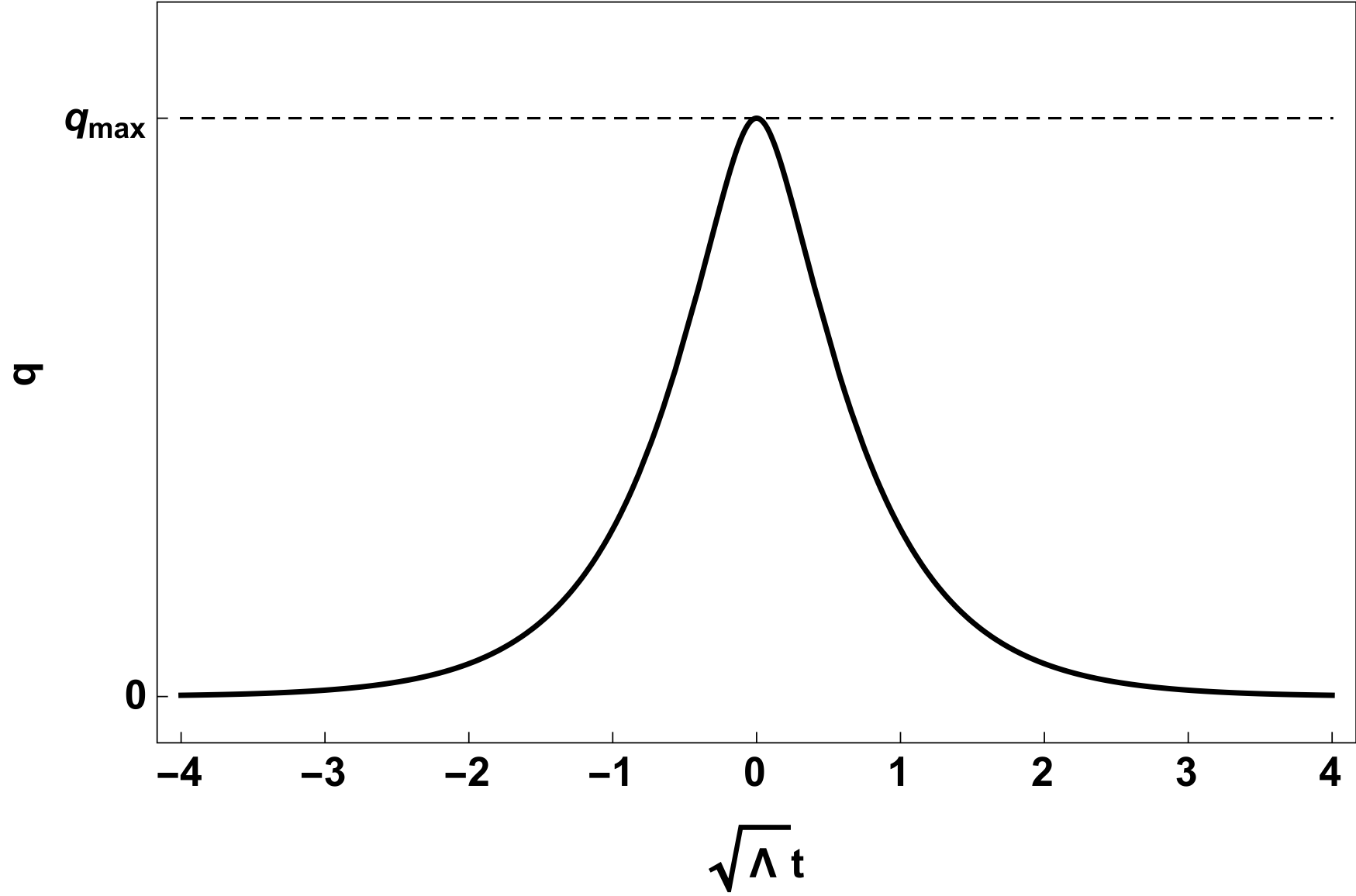 Figure 1
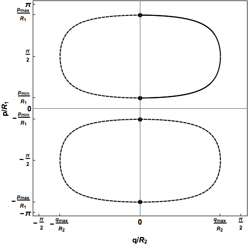 Figure 2
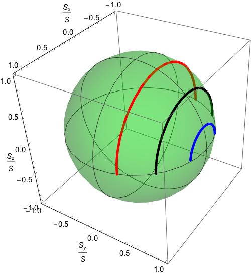 Figure 3
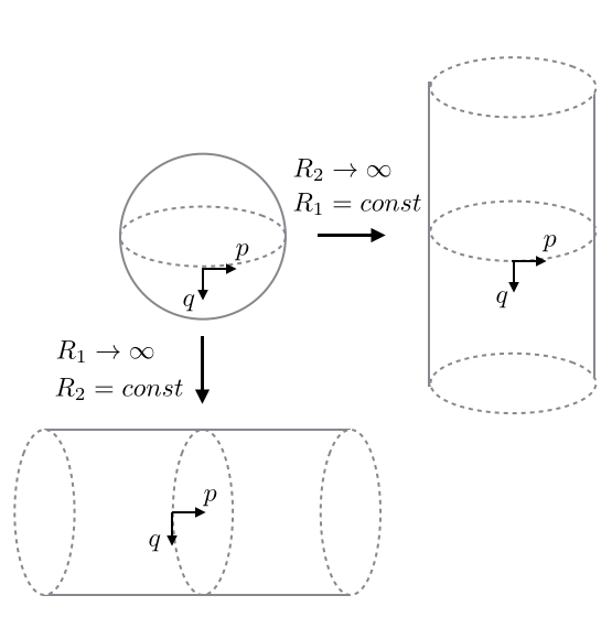 Figure 4
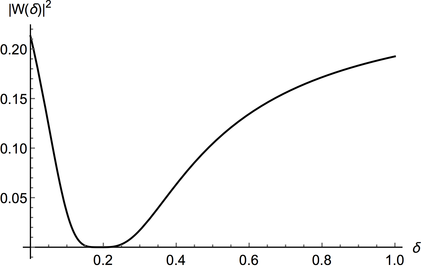 Figure 5
Peer Reviews
No public reviews on file for this paper yet. If you reviewed it on a platform where reviews are public (OpenReview, ICLR, NeurIPS, ICML), you can paste yours below so the community can read it here.
Videos
No videos yet. Explain this paper in a talk, walkthrough, or lecture? Add one.
Version accepted for publication in Phys. Rev. D.
Minisuperspace model of compact phase space gravity
Danilo Artigas*∗,‡*
Jakub Mielczarek*∗,†*
Carlo Rovelli*∗*
∗Aix Marseille Université, Université de Toulon, CNRS, CPT, 13288 Marseille, France
‡Magistère de Physique Fondamentale, Univ. Paris-Sud, Univ. Paris-Saclay, 91405 Orsay, France
†Institute of Physics, Jagiellonian University, ul. Łojasiewicza 11, 30-348 Kraków, Poland
Abstract
The kinematical phase space of classical gravitational field is flat (affine) and unbounded. Because of this, field variables may tend to infinity leading to appearance of singularities, which plague Einstein’s theory of gravity. The purpose of this article is to study the idea of generalizing the theory of gravity by compactification of the phase space. We investigate the procedure of compactification of the phase space on a minisuperspace gravitational model with two-dimensional phase space. In the affine limit, the model reduces to the flat de Sitter cosmology. The phase space is generalized to the spherical case, and the case of loop quantum cosmology is recovered in the cylindrical phase space limit. Analysis of the dynamics reveals that the compactness of the phase space leads to both UV and IR effects. In particular, the phase of recollapse appears, preventing the Universe from expanding to infinite volume. Furthermore, the quantum version of the model is investigated and the quantum constraint is solved. As an example, we analyze the case with the spin quantum number , for which we determine transition amplitude between initial and final state of the classical trajectory. The probability of the transition is peaked at .
I Introduction
Compact phase spaces emerge in the semiclassical description of a quantum system with finite dimensional Hilbert spaces. An important property of compactness is that values of phase space variables are bounded. As a consequence, physical quantities such as energy density may be constrained from above, resolving the problem of divergences appearing in the case of affine phase spaces. Compactification of phase spaces may, therefore, serve as a way to impose the principle of finiteness, introduced by Max Born and Leopold Infeld Born:1934fy .
Following this reasoning, in Ref. Mielczarek:2016rax a research program of nonlinear field space theory (NFST) has been initiated with the goal of generalizing the known types of physical fields to the case of compact phase spaces. In the original article Mielczarek:2016rax the procedure of compactification has been investigated at the level of the Fourier space representation of a scalar field theory. For the standard scalar field, each Fourier mode is associated with a two-dimensional phase space, which in the NFST has been considered as a local approximation to the spherical phase space . The procedure has been thereafter applied for the field defined in the position space in Ref. Mielczarek:2016xql . It has been shown that, thanks to the fact that the spherical phase space is a phase space of angular momentum (spin), a new possibility of relating spin systems with field theories emerges. In particular, it has been shown in Ref. Mielczarek:2016xql that small excitations of the continuous version of the Heisenberg model are described by nonrelativistic scalar field theory, if the large spin limit () is considered. Furthermore, the scalar field theory recovered satisfies the so-called Born reciprocity symmetry between generalized positions and conjugate momenta Born49 . Worth mentioning is that, while the Born reciprocity has mostly been forgotten for years because of its incompatibility with relativistic symmetries, it has recently reemerged in the context of string theory and quantum gravity Freidel:2013zga ; Freidel:2014qna .
The next step of the NFST program was to show that the construction can be generalized to the case of relativistic Klein-Gordon scalar field theory Bilski:2017gic . It was demonstrated that such theory is recovered in the large spin limit of the XX Heisenberg model (XXZ Heisenberg model in the limit of the vanishing anisotropy parameter ). Possible consequences of the compact phase space scalar field theory have been investigated in the cosmological context, by applying the compactness to the inflationary scalar field Mielczarek:2017ny . It has been shown that the compactness of the inflaton field may have implications on amplitudes of cosmological primordial inhomogeneities as well as leading to the phase of cosmological recollapse Mielczarek:2017ny .
While the case of scalar field theory is a good testing ground for the procedure of compactification of the phase spaces, the ambition of the NFST is to ultimately apply the method to the gravitational interactions. The expectation is that compact phase space extension of general relativity (GR) may resolve the problem of singularities (simply by restricting field variables to take finite values) and pave a way to a finite Hilbert space quantum version of the theory of gravity. A possibility of such an approach to quantum theory of gravity has already been discussed in the context of loop quantum gravity (LQG) in Ref. Rovelli:2015fwa . In the current formulation, LQG is a theory with phase space per link of the spin network. Part of the phase space, associated with the holonomies is already compact. However, the remaining contribution is affine and is described by elements of the algebra. The idea pushed forward in Ref. Rovelli:2015fwa was that generalization of the theory to the compact phase space may resolve certain problems (e.g. IR divergences) present in the current formulation. Furthermore, nontrivial phase spaces are considered in the relative locality approach to quantum gravity AmelinoCamelia:2011bm . However, at the current stage of development, the phase space of particles rather than field (including gravitational field) is considered in this approach.
The purpose of this article is to make a step towards construction of the compact phase space version of GR by studying the procedure of compactification of the gravitational degrees of freedom in a minisuperspace model. More specifically, our objective is to introduce phase space compactness to the flat Friedmann-Robertson-Walker (FRW) cosmological model with positive cosmological constant . There is of course a freedom of choices of possible compact phase space extensions of initial affine phase space theory. In our studies, we explore the spherical phase space, which will allow us to build relations with the spin physics. However, in general, other possibilities, such as toroidal phase space , can also be considered.
We study the classical and the quantum theory for which exact analytical solutions are found. We show that loop quantum cosmology is recovered in a certain limit. We demonstrate how transition amplitude can be explicitly computed in the quantum theory using the projector onto solutions of the quantum Hamiltonian constraint and coherent boundary states in the kinematical Hilbert space.
The organization of the article is as follows. In Sec. II we introduce the standard de Sitter model and notation used through this article is established. Then in Sec. III the spherical phase space is introduced and the affine large spin limit at the kinematical level is discussed. Based on this, in Sec. IV the standard FRW dynamics with positive cosmological constant is generalized to the case with compact phase space. The Hamiltonian constraint we obtain is expressed in terms of the spin variable, which parametrizes the phase space. In Sec. V we show that the theory reduces to loop quantum cosmology if the phase space is elongated in the direction of one of the canonical variables. This yields a cylindrical phase space. In Sec. VI we derive analytical solutions of the full model. The quantum analysis of the model is performed in Sec. VII, where the quantum constraint is explicitly solved and exemplary transition amplitudes associated with end points of the classical trajectory are calculated. The results are summarized in Sec. VIII.
II de Sitter model
The phase space is a symplectic manifold equipped with closed 2-form . In the case of the FRW cosmology, can be written in the Darboux form
[TABLE]
where is the generalized coordinate and is the canonically conjugated momentum. is a volume element, related to the scale factor and fiducial volume as follows: . Keeping in mind different possible triad orientations, we allow both positive and negative real values of . As a consequence, the phase space for the system is .
In terms of the and variables, the Hamiltonian for the flat FRW cosmology with cosmological constant takes the form Mielczarek:2017ny
[TABLE]
where and is the lapse function. is the Planck length.
By inverting the symplectic form (1) the Poisson bracket
[TABLE]
can be introduced, where and are phase space functions. The Poisson bracket allows us to introduce the Hamilton equation . In the cosmological context it is useful to introduce the Hubble factor , which quantifies the rate of cosmological expansion.
[TABLE]
where the time derivative of is defined in terms of the Hamilton equation . Fixing, from now on, the gauge , we can express the Hubble factor as follows:
[TABLE]
Plugging this relation into the scalar constraint, we have
[TABLE]
and the Friedmann equation in the well-known form
[TABLE]
is recovered, with exponential solutions for .
III Spherical phase space
For the spherical phase space the natural candidate for the symplectic 2-form is the area form,
[TABLE]
where and are spherical angles and has been introduced for dimensional reasons. The volume (area) of the phase space is now finite and equal to
[TABLE]
The affine limit corresponds to . As showed in Ref. Mielczarek:2016xql , it is convenient to perform a change of coordinates in the form:
[TABLE]
such that the 2-form (8) rewrites as
[TABLE]
where we have set that . This guarantees that in the large limit (), the symplectic form (12) simplifies to the case with symplectic form (1). The form (12) differs from the one introduced in Ref. Mielczarek:2016xql by the change of variables , which does not change physics but the convention used here allows us to make direct connection with polymerization of momentum . Based on the symplectic form (12), the Poisson bracket becomes
[TABLE]
The difference with the case (3) is the presence of the factor . Both the and variables are only locally well defined on the sphere, but it is justified to introduce globally defined functions to study the dynamics also away from the origin of the coordinate system . A choice that guarantees that the new variables are globally defined and the algebra of the variables takes a simple form is associated with the parametrization of the sphere in a Cartesian coordinate system. Namely, we introduce a vector , with components expressed in terms of the and variables as follows:
[TABLE]
Differentiating the components with respect to the and variables we get
[TABLE]
and
[TABLE]
when applied to the Poisson bracket (13), we find that the components satisfy the algebra
[TABLE]
The vector is therefore a vector of angular momentum (spin) with magnitude equal to . The affine limit is, therefore, a large spin limit.
IV Compact phase space FRW model
In the previous section we have shown that, at the kinematical level, compactification of the affine phase space of the FRW model to the case of can be performed replacing the symplectic form (1) with (12). The second step is to introduce the compactness at the level of the dynamics, by suitable modification of the minisuperspace Hamiltonian (2). Since the original and phase space variables are not globally defined on the sphere, we have to replace them with the variables introduced in the previous section. The consistency requirement is that in the large spin limit () the classical FRW Hamiltonian (2) would be recovered. We take here the additional requirement that in the limit the case of the polymer quantization is recovered.
The simplest way to satisfy the above conditions is to perform the following replacements:
[TABLE]
where the new variables are defined such that and . Applying the above replacements in Eq. (2) a new Hamiltonian defined on spherical phase space can be introduced,
[TABLE]
such that in the limit.
The Hamiltonian (22) and the Poisson bracket (13) yield the equations of motion:
[TABLE]
With the use of the set of equations above, one can check that
[TABLE]
Let us now derive the Friedmann equation. For this purpose, using the Poisson bracket (13), we calculate
[TABLE]
so that (fixing as above the gauge ) the Hubble factor (4) takes the following form
[TABLE]
or equivalently
[TABLE]
such that in the limit we recover , as expected [see Eq. (5)].
The condition implies that the scalar constraint takes the form
[TABLE]
which reduces to
[TABLE]
Therefore, the Friedmann equation takes the form
[TABLE]
in the gauge. The real solutions to the equation can be obtained if the condition
[TABLE]
is satisfied, where for convenience we have defined
[TABLE]
V Polymer limit
While the spherical case imposes restrictions on the values of and , we now study the limits where the constraints on the phase space variables are released. This is equivalent to elongating the spherical phase space into a cylindrical shaped phase space, by taking either the or limit (see Fig. 1). The cylindrical phase space obtained corresponds to the so-called polymerization Ashtekar:2002sn , playing a crucial role in loop quantum cosmology (LQC) Bojowald:2008zzb ; Ashtekar:2011ni . A preliminary analysis of the relation between spherical phase space and the polymerization of momentum at the kinematical has been performed in Ref. Bilski:2017gic . Here, we consider the polymer limit in both canonical directions and explore consequences on dynamics.
V.1 Momentum polymerization
We first consider the limit, so that the symplectic form (12) reduces to the Darboux form (1) and the Poisson bracket (13) reduces to the affine case (3). Under this limit, the spin components reduce to
[TABLE]
together with . Based on the algebra, this one reduces to
[TABLE]
which is the cylindrical algebra on the phase space Bojowald:2011jd . If one takes the limit the only nontrivial contribution to the algebra that remains is (39), which simplifies to as expected.
The Hamiltonian of the spherical phase space (22) reduces now to
[TABLE]
where the index denotes that we now deal with cylindrical phase space. We can simplify the Hamiltonian to
[TABLE]
where we have introduced the scale of polymerization , so that in the limit () the FRW Hamiltonian is recovered.
The expression (42) is equivalent to the Hamiltonian of LQC, where we have the following polymerization of the momentum:
[TABLE]
such that .
In the limit, the Friedmann equation (32) simplifies to
[TABLE]
for , and a real solution to the equation can be found only if . Hence, the dynamics imposes bounds on the possible values of cosmological constant. This effect has already been noticed before in the polymerized cosmology Mielczarek:2008zv ; Mielczarek:2010rq ; Mielczarek:2010wu .
Using the expression for the energy density of the cosmological constant , the Friedmann equation (44) can be rewritten as
[TABLE]
where the is the critical energy density considered in LQC,
[TABLE]
The leading contribution in Eq. (45) matches with the Friedmann equation for a flat phase space (7), whereas the second contribution implies correction to the cosmological evolution due to the cylindrical phase space. Equation (45) has a solution in the exponential form
[TABLE]
where we have introduced an effective cosmological constant .
V.2 Position polymerization
We now proceed as above, but considering the limit. The symplectic form associated to a spherical phase space is unchanged, and so is the corresponding Poisson bracket, while the spin components reduce to
[TABLE]
The algebra reduces to
[TABLE]
which is different from the cylindrical algebra because of the presence of the nonvanishing factor in the symplectic form (12). However, if instead of the variable one considers given by Eq. (21), the symplectic 2-form (12) can be expressed in a Darboux form
[TABLE]
and we obtain , which agrees with (52).
Rewriting the Hamiltonian (22) under this limit gives
[TABLE]
Regarding the Friedmann equation, we can put Eq. (28) under the form
[TABLE]
An exact solution to this equation can be found again,
[TABLE]
where is a constant of integration.
VI Cosmological evolution
The aim of this section is to study the consequences of the modified Friedmann equation (32) obtained in the case of the spherical phase space. The equation can be rewritten in the form of the integral
[TABLE]
where . The integral can be performed leading to
[TABLE]
where is a constant of integration that, without loss of generality, can be fixed as . The solution is then symmetric with respect to the mirror symmetry and by examining the limits of Eq. (59) we find that in the limits the value of tends to its minimal value,
[TABLE]
On the other hand, at the value of reaches (or symmetrically ), where
[TABLE]
There are two symmetric branches of solution, related by the mirror symmetry . The solution has a form of recollapsing universe with asymptotical de Sitter solutions at with the effective cosmological constant [given by Eq. (47)]. We present the solution in Fig. 2. A qualitatively similar solution has been studied in the context of quantum reduced loop gravity Cianfrani:2015oha .
In Fig. 3 we show phase trajectories corresponding to the dynamics. Because the kinematical phase space is two-dimensional, by imposing the constraint the physical subspace is just one-dimensional subspace (curve). In this figure, the solid line represents the trajectory associated with the solution shown in Fig. 2 and positive values of .
The other three symmetric solutions, obtained by applying the reflections and , are shown as the dashed lines in Fig. 3 (for the same value of ). The black dots represent beginning and ends to the trajectories, corresponding to times . They are located at the equator of the phase space, where .
While the reaches its maximal value, the canonically conjugated variable tends to either or (for a symmetric solution) to . The minimal positive value of , associated with the ends of the trajectory is
[TABLE]
and the maximal value is
[TABLE]
Based on Eq. (32), the leading -dependent correction to the Friedmann equation is
[TABLE]
Because , the leading correction scales as . We can define an effective energy density,
[TABLE]
Using the continuity equation,
[TABLE]
we find that the Universe behaves effectively as filled by a fluid with effective pressure
[TABLE]
The effective equation of state implied by the compact nature of the phase space is
[TABLE]
where the equation of state for the effective cosmological constant remains in the classical form . The barotropic index for the correction is , which can be interpreted as a special kind of the phantom matter Caldwell:1999ew .
VI.1 Evolution of the vector
Let us now discuss evolution of the three spin components . Because of the scalar constraint (30), which can be written in the form
[TABLE]
the equations of motion (23-25) (on the surface of the constraint) can be written as
[TABLE]
with const. Because of the equation of the sphere , only one independent differential equation remains,
[TABLE]
where . The analytical solution to Eq. (73) can be found leading to
[TABLE]
There are four symmetric solutions for the four quadrants of a sphere. In the solution with two pluses, as time flows, the component grows from to , while the remains constant. The component grows from [math] to its maximal value and then is decreasing again to [math].
VII Quantum theory
In the quantum theory the Hamiltonian (22) is promoted to an operator . The appropriately symmetrized111For simplicity, we do not decompose and do not include factorial powers of the operators in the symmetrization. and normalized constraint can be written as
[TABLE]
The task is now to find the physical states belonging to the kernel of the operator, i.e., .
A convenient method to deal with constrained systems is the group averaging Ashtekar:1995zh ; Giulini:1999kc . We introduce the projection operator (see, e.g., Rovelli:2009tp ),
[TABLE]
which projects to the zero eigenvalue of the operator . The operator projects quantum states onto the physical subspace and satisfies the condition .
We are mostly interested in the large spin limit () in which the semiclassical cosmological behavior can be reconstructed. In that case, the area of the phase space is large and the and variables are well defined.
It is important to stress that there are two ways of looking at the minisuperspace model. The first is that the model provides description of the Universe at the largest possible (cosmological) scale, describing averaged degrees of freedom. However, there is also a second interpretation, which is especially interesting in the Belinsky-Khalatnikov-Lifschitz Belinsky:1970ew ; Belinsky:1982pk limit characterized by decoupling off the space points. In this case, evolution at each space point is described by a homogeneous (in general anisotropic) minisuperspace model. Furthermore, by introducing interactions between the minisuperspace models at points, one can try to study spatial properties of the field configuration Baytas:2016cbs . From this perspective, the small spin case can have relevance for the very early Universe, before the semiclassical regime has been entered. Therefore, let us start our consideration with the simplest case of spin .
VII.1 Spin 1/2
In this case, the spin components are expressed as
[TABLE]
where are Pauli matrices and . Therefore, and the spherical phase space has an area operator . The scalar constraint (77) reduces to
[TABLE]
defining . We directly conclude that there are no physical states in this case: dim. This is because , where does not have nontrivial solutions. In agreement with this, the projector operator is null,
[TABLE]
VII.2 General spin
Let us now proceed to the general quantum number . In order to find matrix elements of the constraint in the basis , where , it is useful to introduce spin ladder operators,
[TABLE]
The action of the relevant spin operators on the states is given as follows:
[TABLE]
And from Eq. (16), we see that the eigenvalues correspond to eigenvalues of the quantum 3-volume. Applying the above formulas to Eq. (77), we find the matrix elements
[TABLE]
where denotes the Kronecker delta, and the coefficients are defined as
[TABLE]
where we notice the following properties:
[TABLE]
And reduces then to an antipersymmetric Hankel matrix with only three nonzero diagonals.
For the particular case , and are not defined, and , which is in agreement with Eq. (80).
An important property of the matrix
[TABLE]
is that its determinant is always equal to [math] only for bosonic representations (). For the fermionic representations with half integers () the determinant is some function of and can be equal to [math] only for some special values of . As a consequence, for arbitrary there are nontrivial vectors belonging to the kernel of the matrix only in the bosonic case. Furthermore, the matrix is symmetric and therefore has real eigenvalues.
VII.3 Solving the quantum constraint
The general solutions of the constraint equation
[TABLE]
can be expressed in terms of the basis states as follows:
[TABLE]
together with the normalization condition . With the use of the matrix elements, we obtain the following recursive equation
[TABLE]
for , together with
[TABLE]
Combining these conditions together and using Eq. (92), we get the following conditions:
[TABLE]
We can now prove by recurrence that, for any ,
[TABLE]
which allows us, using another recurrence, to show that
- •
for the bosonic case , ,
[TABLE]
- •
for the fermionic case , ,
[TABLE]
Let be an arbitrary matrix with for the bosonic case or for the fermionic one, . The matrix determinant can be represented as
[TABLE]
By property of the linear alternating form of the determinant, we can exchange columns by pairs and do the same with rows to rewrite
[TABLE]
Using the properties of Eq. (88), we finally get
[TABLE]
Therefore, in the bosonic case (odd ), the determinant is always [math], ensuring that at least one eigenvalue is equal to [math].
From this we conclude that for bosons, in the eigenbasis of the projection operator can be written as
[TABLE]
where we have the components originating from each (degenerated) eigenvalue equal to [math] in , whereas any eigenvalue implies a component in the diagonalized projection operator. Therefore, as long as the projection operator is non-[math], there exists a nontrivial solution to equation .
In the fermionic case, nontrivial solutions may exist only for certain values of the parameter . In particular, for there are no nontrivial solutions (except in the case for which the constraint is identically equal to [math]), for nontrivial a solution exists for , and for there are two values for which the determinant of is vanishing: and . Every further case has to be investigated individually.
VII.4 Example:
As an example of the solution of the constraint let us examine the case of . In this case the constraint takes the following matrix form:
[TABLE]
For , there is a single state that satisfies the constraint and is given by
[TABLE]
where appropriately normalized coefficients are
[TABLE]
On the other hand, for , the constraint has three linearly independent solutions:
[TABLE]
The matrix (109) can be diagonalized so that , where the diagonal matrix , where the eigenvalues
[TABLE]
With the use of this, the exponentiation of the constraint can be written as
[TABLE]
As a consequence, the projection operator takes the form
[TABLE]
in the case. The factor in the middle matrix comes directly from the eigenvalue, whereas any eigenvalue implies a component in the projection operator.
Using the expression of , the projection operator finally reads
[TABLE]
in the case, where we defined
[TABLE]
The form of the projection operator we have obtained agrees with the expression given as a dyadic product of the physical states , i.e.,
[TABLE]
taking the physical state given by Eq. (110). The property is satisfied in a consequence of the proper normalization of the state .
If we consider the degenerated case with , for which , the projection operator reads
[TABLE]
where the states for are given by Eqs. (113)-(115).
Let’s now take arbitrary and consider sequences from an initial state to a final state , together with the transition amplitudes . From the expressions of (130) we directly observe that states and do not belong to the sequence if . For the basis states, the transition amplitudes are
- •
each time we transit from to where (i.e. the state is possibly unchanged).
- •
each time we transit from to and vice versa, or from to and vice versa.
- •
each time the state is unchanged.
- •
each time the states and remain unchanged for the case.
In Sec. VI we have shown that the cosmological evolution from to is associated with the rotation of the spin vector from the position
[TABLE]
to
[TABLE]
See the bolded trajectories in Fig. 4. There are also symmetric solutions in the three other quarts of the sphere, but let us now focus on this representative one. Namely, we want to find what is the quantum transition amplitude associated with this evolution as a function of the parameter ,
[TABLE]
for the case, considered in this section. At the level of quantum mechanics, the boundary conditions (148) and (149) translate into the properties of the mean values of the components of the spin operator in the initial and final states, i.e.
[TABLE]
and
[TABLE]
where for the case considered, . Furthermore, it is assumed that dispersion relations are minimized, which is satisfied by coherent states. These can be obtained by rotations of the state into directions of the vectors (148) and (149). An appropriate rotation operator takes the form
[TABLE]
where and are the spherical angles introduced in Sec. III. What is to be performed is the rotation of the state (for which the spin vector is precessing around the axis) first by angle around axis (using the operator ). This aligns the vector to the plane. Then we rotate the vector around the axis (using the operator ) to the initial and final orientations of the spin vector, with and . For both initial and final state, we have and
[TABLE]
Using this, the initial and final states can be written as
[TABLE]
where the coefficients
[TABLE]
where are components of the Wigner -matrices,
[TABLE]
With the use of these results, we obtain the following initial and final states:
[TABLE]
and
[TABLE]
Then, it is straightforward to calculate the transition amplitude (150) using the projection operator given by Eq. (130) for and by Eq. (147) for . For , the final form of the transition amplitude is
[TABLE]
which is a purely real function. In the special case the transition amplitude is . We plot the modulus square of the amplitude in Fig. 5.
The probability of transition is maximized for , where . Then, the probability is decreasing to [math] at and is increasing to the value at the maximal value of . It is interesting that in the limit of vanishing cosmological constant the probability takes the maximal value.
Let us explore this feature in some more detail. For this purpose, we recall that the probability amplitude (169) describes quantum transition between quantum states peaked at two end points of a classical trajectory (at ). In the considered case of , the associated quantum dynamics is approximated by a five-level quantum system. This, however, does not mean that we are restricted to the Planckian regime only. The maximal volume of the Universe is determined by both and [see Eq. (61)]. The can take arbitrary large values, provided that the relation is satisfied.
For the transition amplitude (169) corresponds to the evolution with , which may describe large scale universe. The fact that a low dimensional quantum system may have cosmological relevance not only at the Planck scale has already been used in spin-foam cosmology, where a dipole spin network provides an approximate large scale description of a universe Bianchi:2010zs ; Vidotto:2010kw . However, in order to recover semiclassical behavior, large spin limit (of spin labels) has to be taken. Accordingly, in our case, correspondence with classical results is expected in the limit (equivalent to the affine limit of a spherical phase space). An open question is whether the main features of the transition amplitude (169) are preserved in this limit. This, however, requires further analysis and cannot be simply answered based only on the studies made here. Worth emphasizing is also that determination of for may also allow one to reconstruct semiclassical action corresponding to the quantum system under consideration. It would be very interesting to check if the effective Friedmann equation (32) is recovered.
VIII Summary
The research program of NFST aims at generalizing the known types of field theory to the case of compact phase space. This goal has already been achieved in the case of scalar field theory.
The aim of this program is the compactification of the phase space of gravity. Thanks to the compactness of the phase space, the field variables become constrained, which may eliminate singularities. The compactness of the phase space is a consequence of the finite dimensionality of the Hilbert space. Therefore, the compact phase space of gravitational field theory is expected to be associated with a quantum theory of gravity characterized by finite number of basis states. In this article, we have examined the possibility of compactifying a minisuperspace gravitational model with a single degree of freedom - a scale factor.
We have focused our attention on the vacuum case with positive cosmological constant. The phase space has been generalized from the affine case to a spherical phase space . This choice has been suggested by the fact that the spherical phase space is a phase space of angular momentum (spin). This enabled us to describe kinematics and dynamics of the model in terms of the angular momentum (spin) vector , the components of which satisfy the () algebra. The affine case is recovered in the large spin limit . At the quantum level, the large spin limit is known to be associated with semiclassical limit, which is consistent with our discussion.
We have investigated semiclassical dynamics of the system and we have derived the modified Friedmann equation. The ambiguity associated with introduction of the compact phase space extension of the Hamiltonian has been reduced by requirement that the known case of loop quantum cosmology with cylindrical phase space is recovered in the limit . In such a case, the so-called polymerization of the momentum , with the polymerization scale , is obtained.
Furthermore, equations of motion for the minisuperspace model with the spherical phase space can be solved analytically. Analysis of the solutions confirmed that both UV and IR results are expected due to compactness of the phase space (see also discussion in Ref. Nozari:2014qja ). The UV effects are associated with the variable (related to the Hubble factor) while the IR effects are associated with the variable (related to the scale factor). In the considered model, manifestation of the IR effects is the maximal possible value of associated with the phase of recollapse of the Universe. On the other hand, the UV effects lead to renormalization of the cosmological constant and existence of their maximal value .
Thereafter, we have analyzed a fully quantum version of the theory and promoted the constraint to be a quantum operator. It turned out that the constraint can be solved recursively for any value of the quantum number . However, the nontrivial solutions exist only in the bosonic case, while in the fermionic case the solutions may exist only for some special values of the cosmological constant . As an example we have analyzed the case with . We have found both physical states (one for and three for ) that satisfy the constraint as well deriving the form of the projector operator . We used the projection operator to evaluate transition amplitude between two coherent states that are associated with the end points of the classical trajectory. We have found that the probability of transition is maximal for .
Some of the future steps in the direction of the research are as follows:
- •
Analysis of the de Sitter model with positive curvature. This can resolve a problem with the interpretation of the IR limit since, in this case, the spatial volume is finite and well defined. Furthermore, the model is expected to lead to oscillatory cosmological evolution.
- •
Analysis of the toroidal compact phase space . This case can be viewed as a symmetry-reduced version of the phase space, being a possible generalization of the loop quantum gravity phase space.
- •
Reconstruction of the physical Hamiltonian. It would be worth reconstructing and studying properties of the physical Hamiltonian associated with the constrained system under investigation. The resulting physical spin Hamiltonian can be used to implement (in laboratory) analog spin models corresponding to the gravitational dynamics under investigation. For this purpose, e.g. tunable magnetic metamaterials with controlled spins could be used. Such systems have been successfully implemented experimentally in the two-dimensional case Louis .
- •
Taking into account matter. Our focus on this article was on the gravitational degrees of freedom and contribution from the cosmological constant has only been taken into account. This needs to be generalized by investigating contributions from different forms of matter. Especially interesting in the cosmological context is the case of a scalar field. Two effects have to be taken into account. The first is an appropriate modification of the scalar field Hamiltonian such that the compactness associated with the variable is introduced in a consistent way. Another issue is the compactness of the scalar field itself. This second issue has be investigated in Ref. Mielczarek:2017ny . However, consistent merging of both types of compactness (gravitational and scalar field) is an open issue to be addressed in future studies.
- •
Semi-classical limit. In Sec. VII the quantum counterpart of the compact phase space minisuperspace model has been introduced and investigated. A physical quantum state belonging to the kernel by the constraint can be found. One can expect that from the state, the classical cosmological dynamics should be recovered in the (semiclassical) large spin limit, . In particular, transition amplitudes between two coherent states in the limit have to be investigated. Furthermore, analysis of the transitions amplitudes should be extended beyond the case of boundaries of a classical trajectory, e.g., to the case of arbitrary two points on the phase space.
Acknowledgements
J. M. is supported by the Sonata Bis Grant No. DEC-2017/26/E/ST2/00763 of the National Science Centre Poland and the Mobilność Plus Grant No. 1641/MON/V/2017/0 of the Polish Ministry of Science and Higher Education.
The reference list from the paper itself. Each links out to its DOI / PubMed record.
- 1(1) M. Born and L. Infeld, Proc. R. Soc. A 144 , 425 (1934).
- 2(2) J. Mielczarek and T. Trześniewski, Phys. Lett. B 759 , 424 (2016), [ar Xiv:1601.04515 [hep-th]].
- 3(3) J. Mielczarek, Universe 3 , 29 (2017), [ar Xiv:1612.04355 [hep-th]].
- 4(4) M. Born, Rev. Mod. Phys. 21 , 463 (1949).
- 5(5) L. Freidel, R. G. Leigh and D. Minic, Phys. Lett. B 730 , 302 (2014), [ar Xiv:1307.7080 [hep-th]].
- 6(6) L. Freidel, R. G. Leigh and D. Minic, Int. J. Mod. Phys. D 23 , 1442006 (2014), [ar Xiv:1405.3949 [hep-th]].
- 7(7) J. Bilski, S. Brahma, A. Marcianò, and J. Mielczarek, Int. J. Mod. Phys. D 28 , 1950020 (2019), [ar Xiv:1708.03207 [hep-th]].
- 8(8) J. Mielczarek and T. Trześniewski, Phys. Rev. D 96 , 043522 (2017).