TL;DR
This paper introduces a new Bayesian computational method to better infer the stellar initial mass function by accounting for observational biases and physical processes, overcoming the limitations of traditional likelihood-based approaches.
Contribution
It develops an approximate Bayesian computation framework incorporating physical models and observational effects for more accurate IMF inference in astronomy.
Findings
Method accurately recovers true posterior in simulations
Accounts for observational limitations and physical processes
Improves inference accuracy over traditional likelihood methods
Abstract
Accurate specification of a likelihood function is becoming increasingly difficult in many inference problems in astronomy. As sample sizes resulting from astronomical surveys continue to grow, deficiencies in the likelihood function lead to larger biases in key parameter estimates. These deficiencies result from the oversimplification of the physical processes that generated the data, and from the failure to account for observational limitations. Unfortunately, realistic models often do not yield an analytical form for the likelihood. The estimation of a stellar initial mass function (IMF) is an important example. The stellar IMF is the mass distribution of stars initially formed in a given cluster of stars, a population which is not directly observable due to stellar evolution and other disruptions and observational limitations of the cluster. There are several difficulties with…
Click any figure to enlarge with its caption.
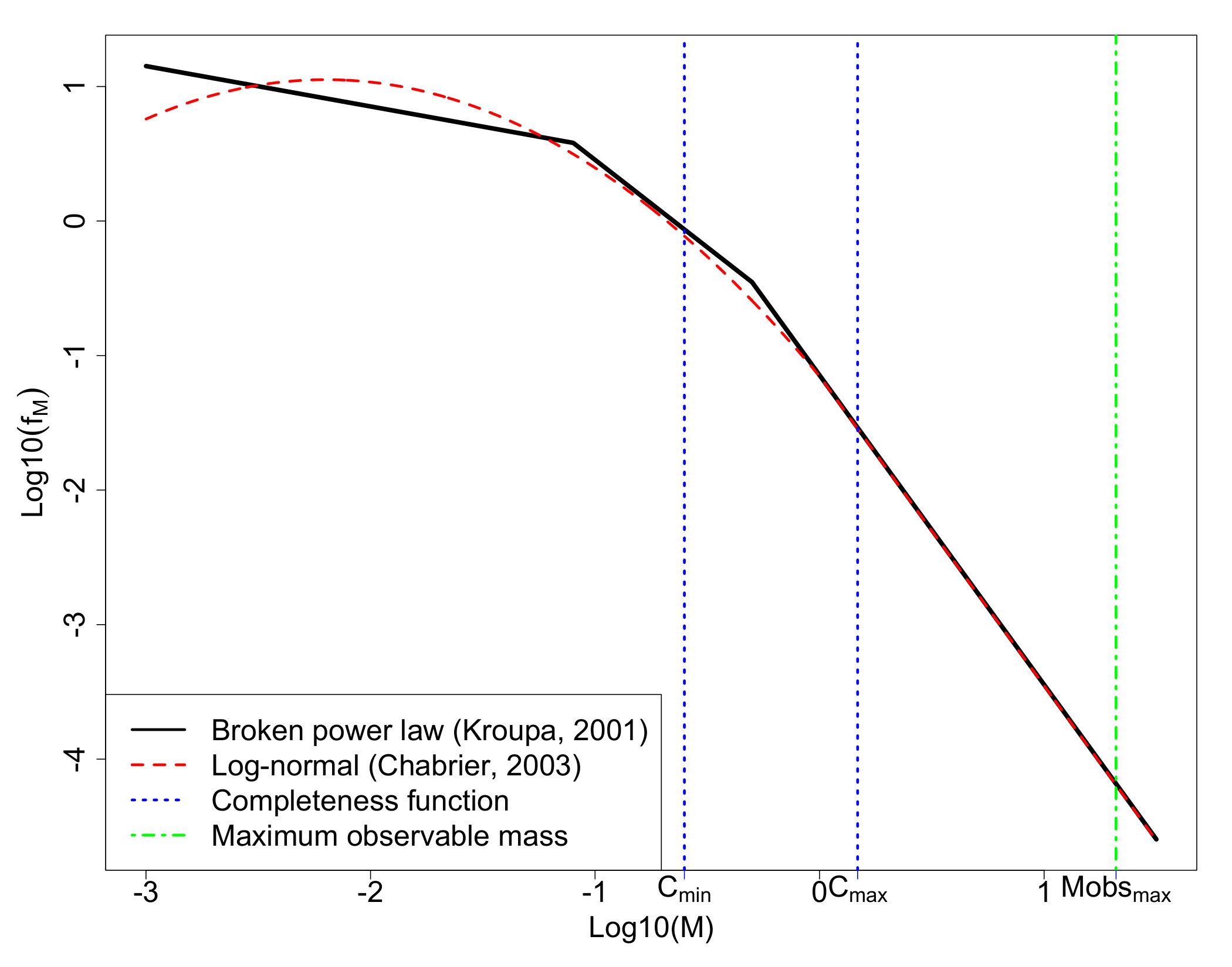 Figure 1
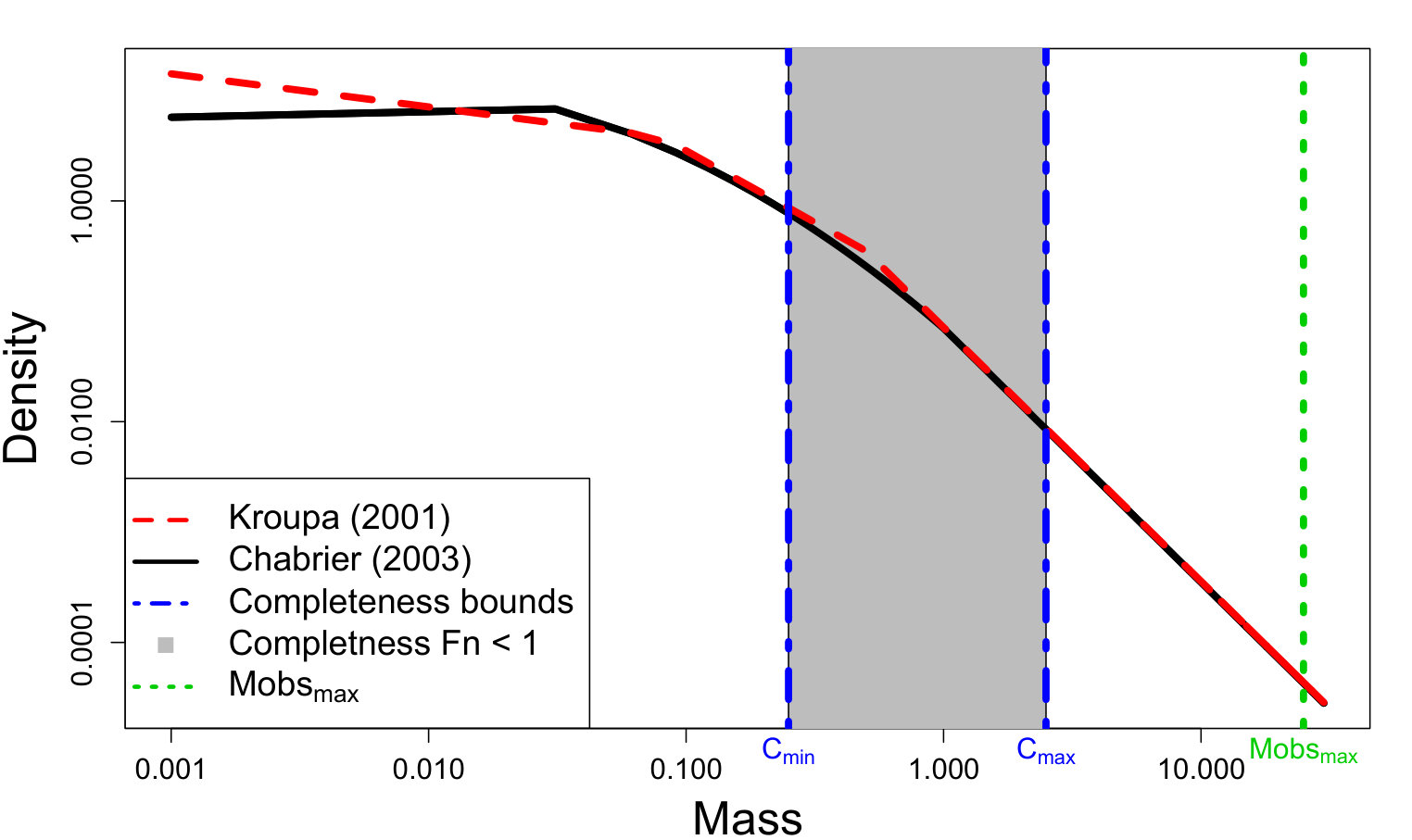 Figure 2
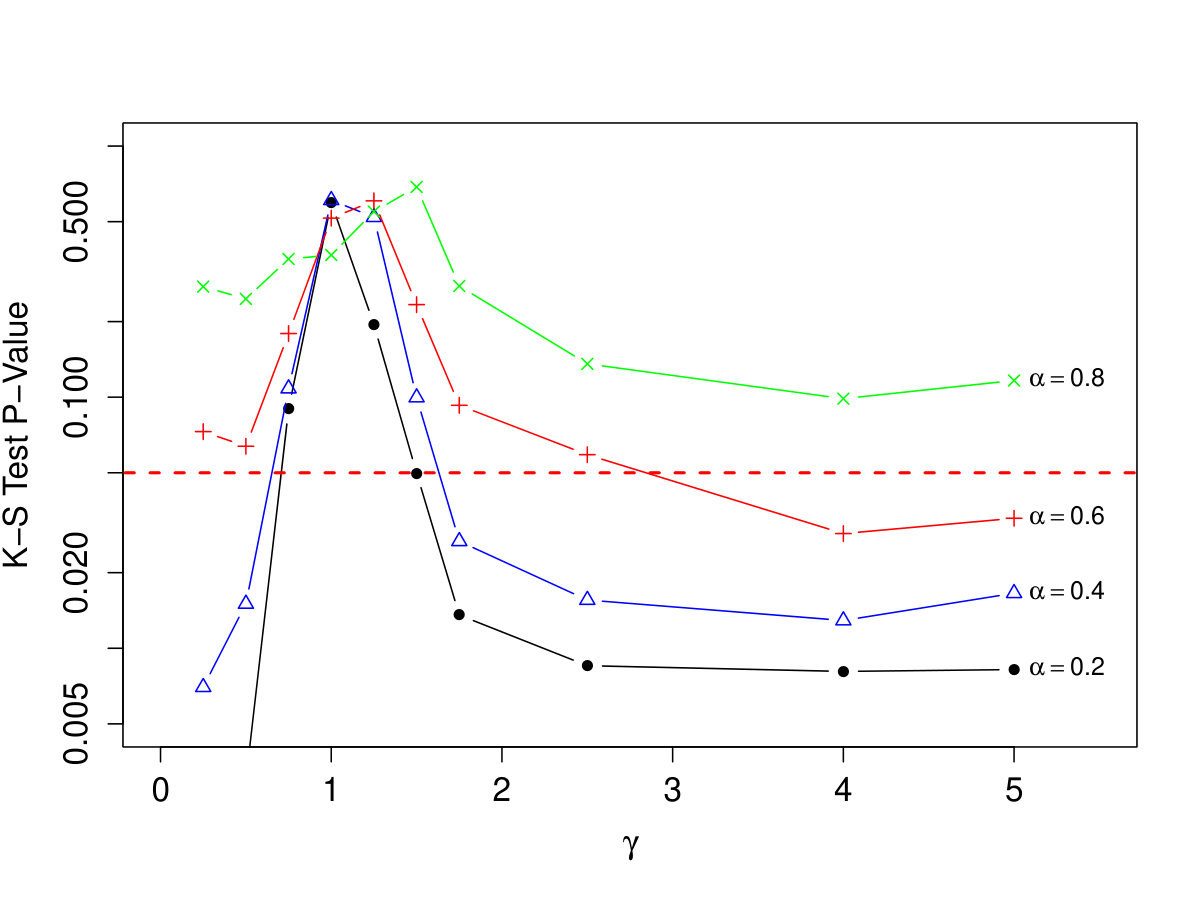 Figure 3
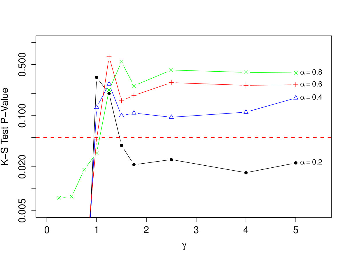 Figure 4
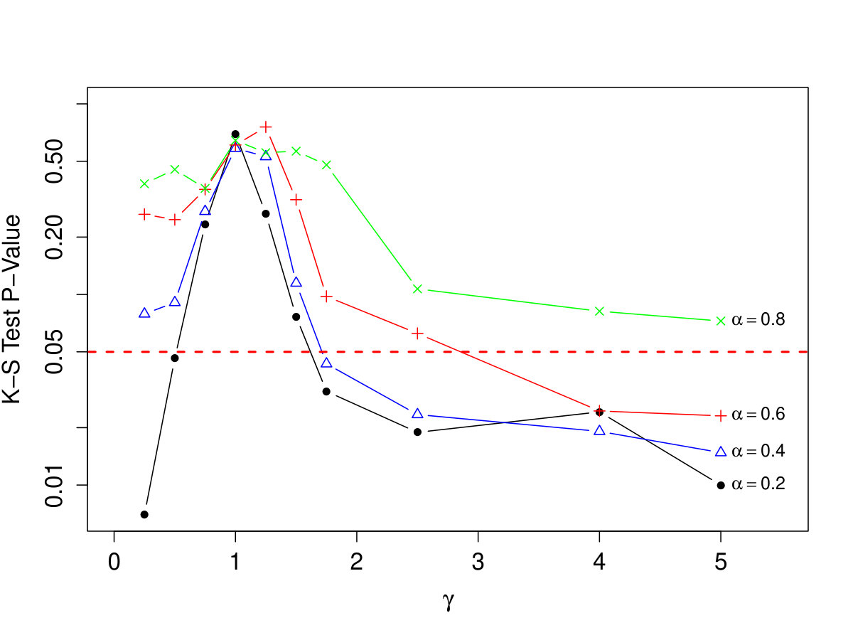 Figure 5
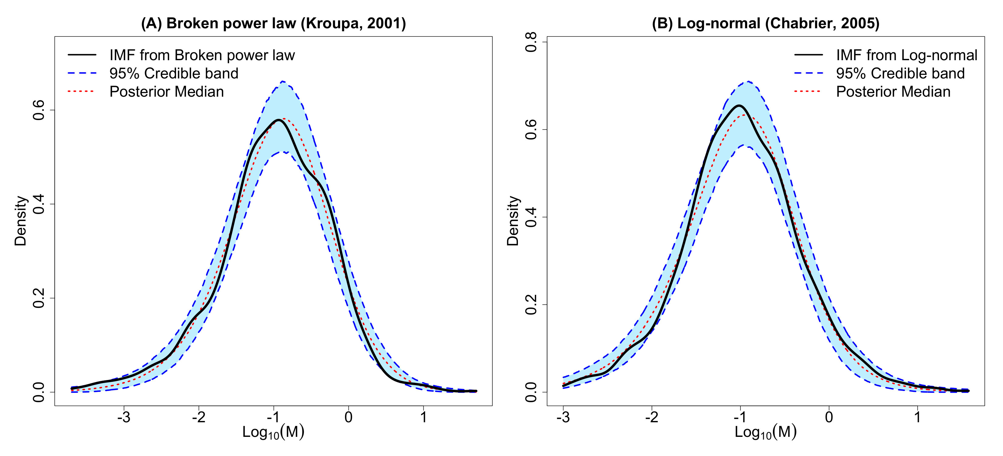 Figure 6
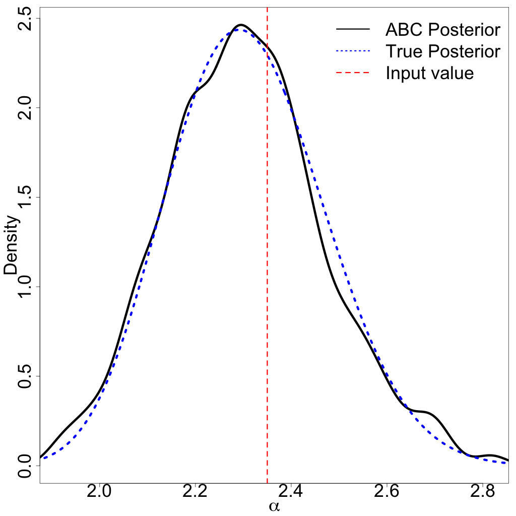 Figure 7
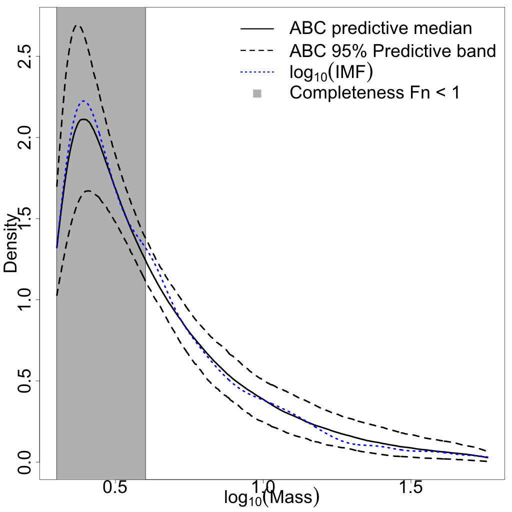 Figure 8
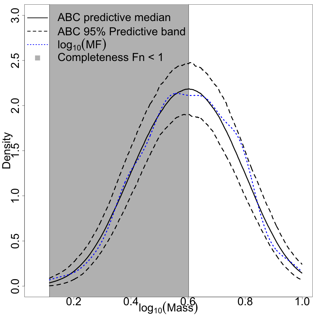 Figure 9
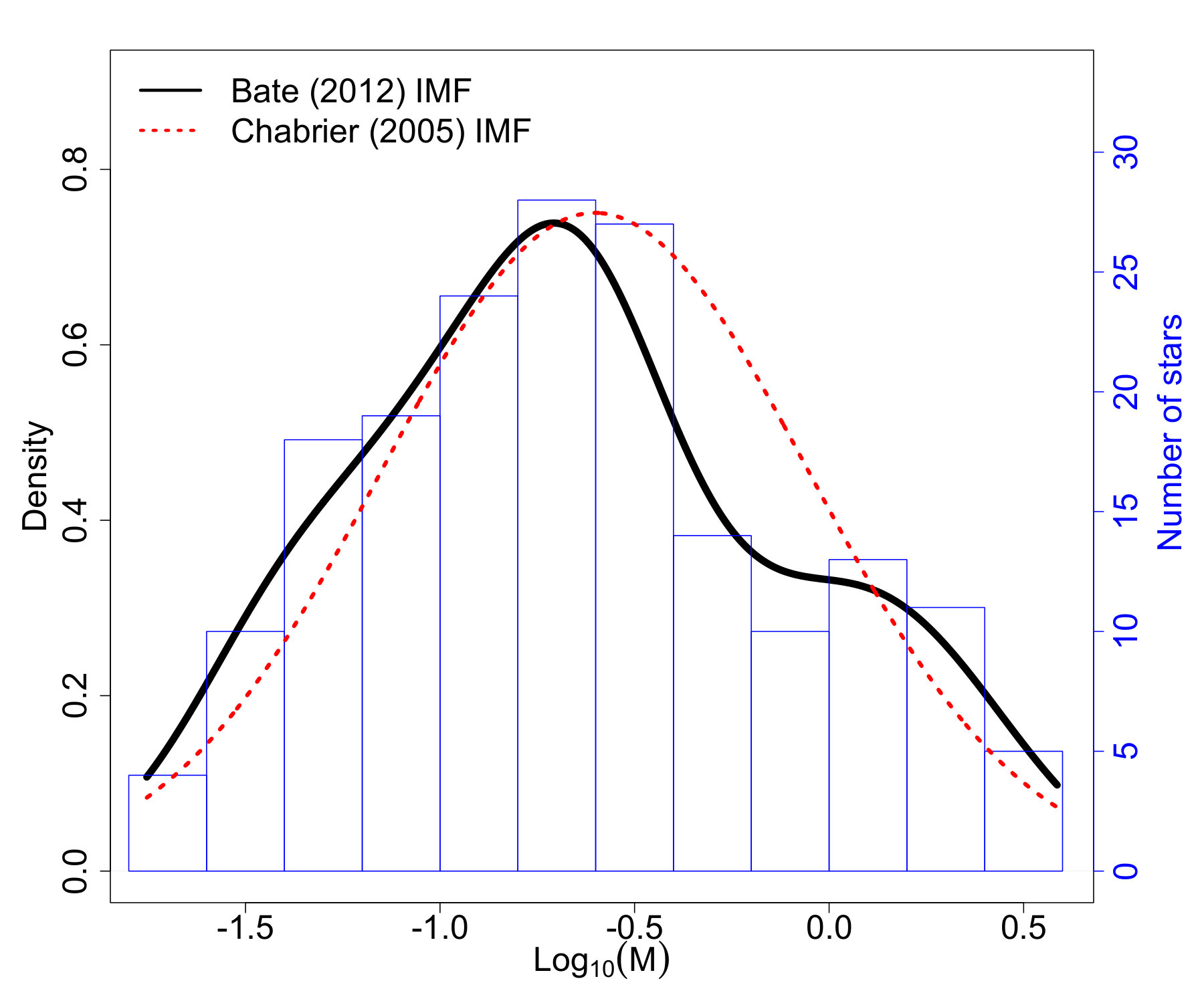 Figure 10
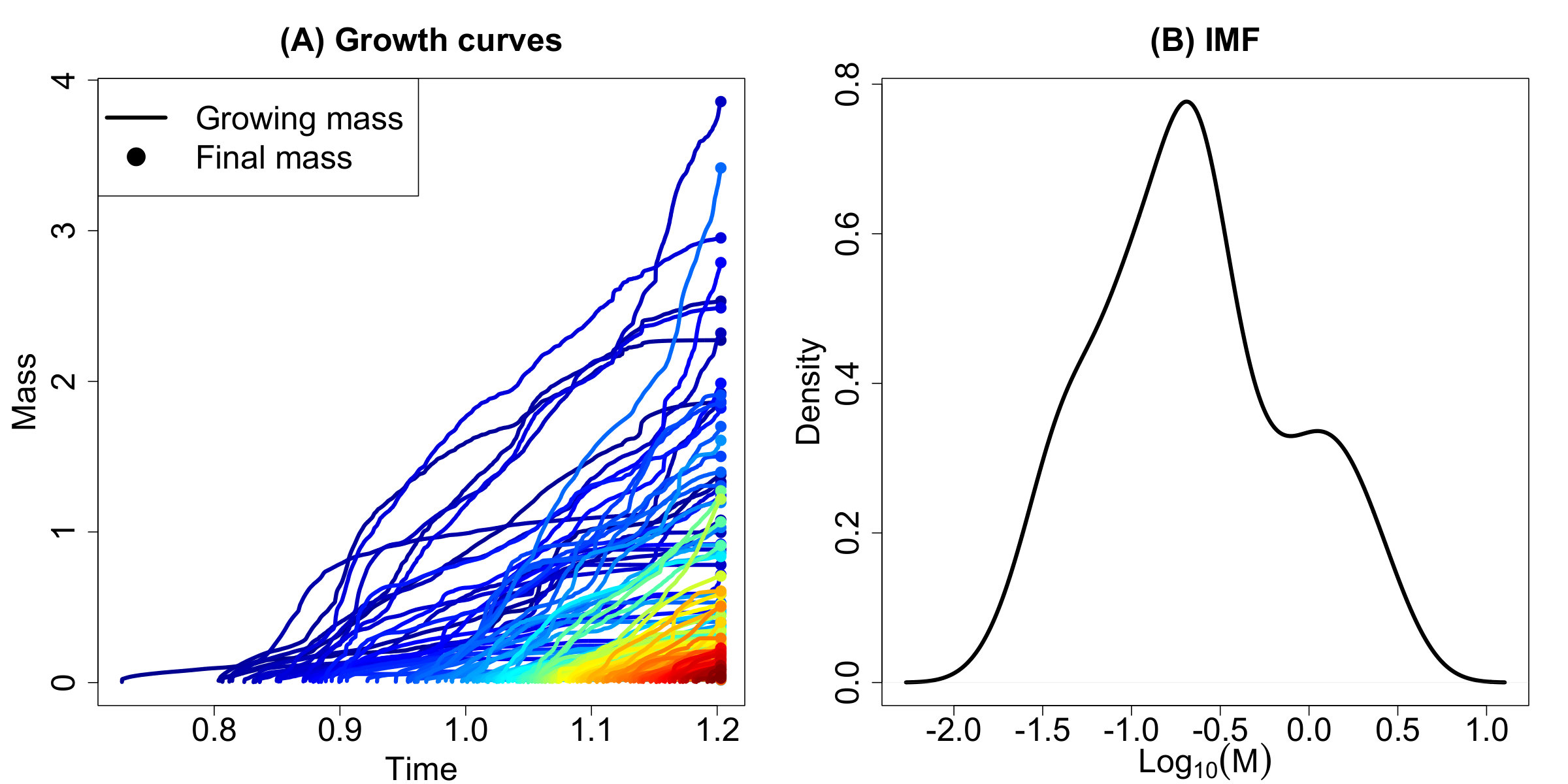 Figure 11
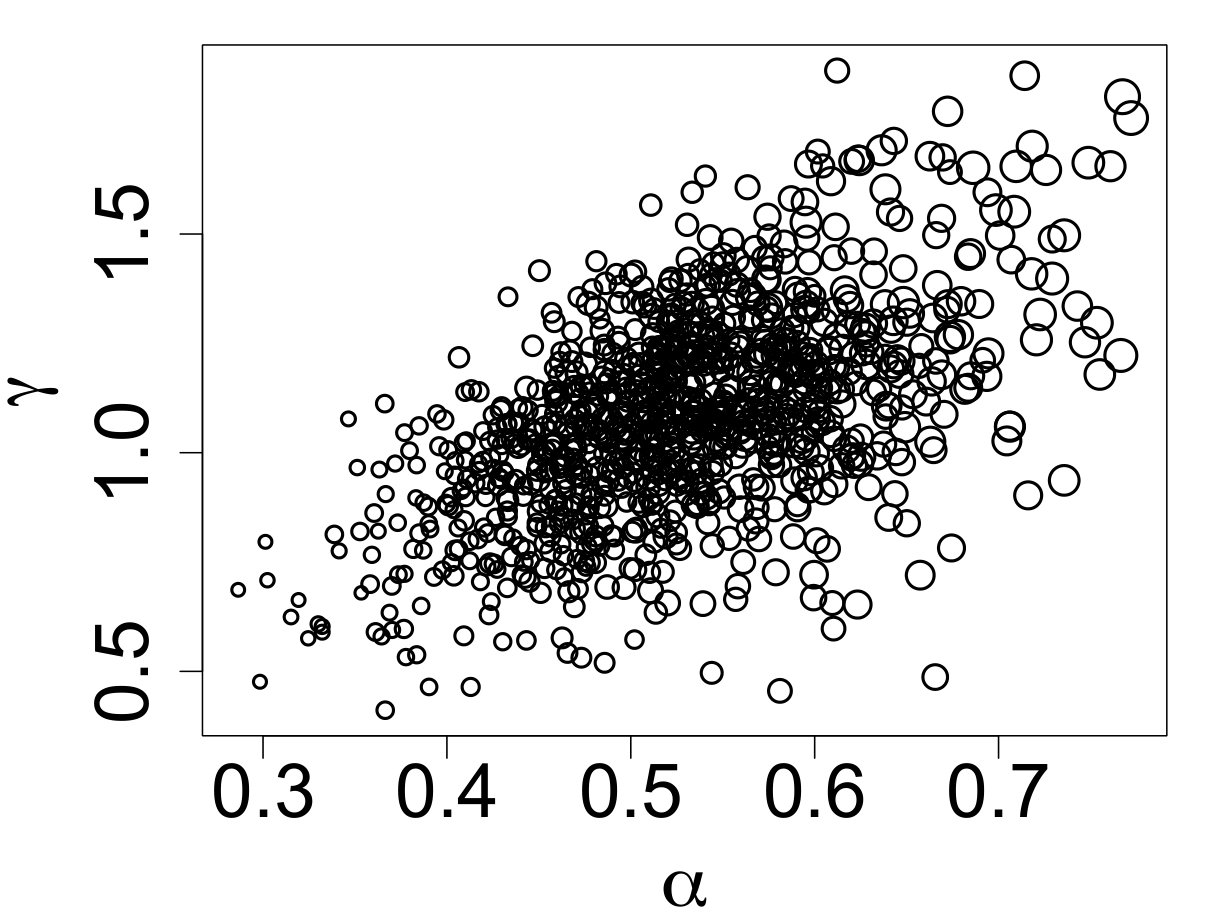 Figure 12
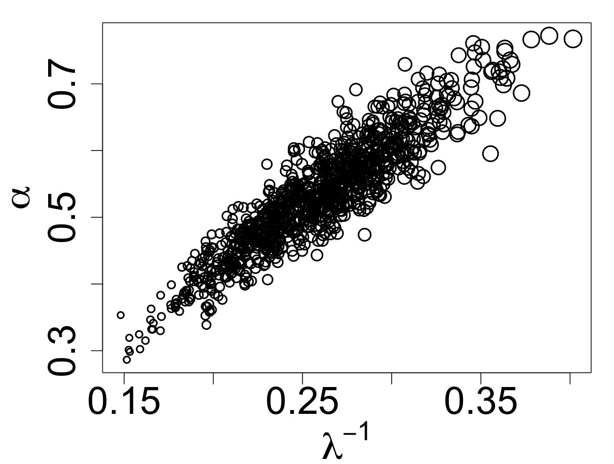 Figure 13
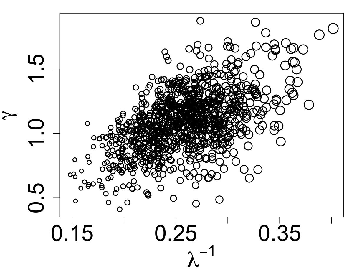 Figure 14
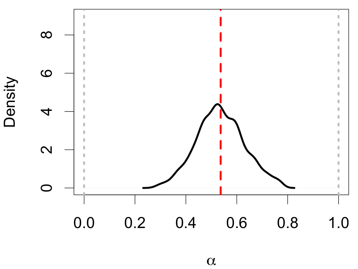 Figure 15
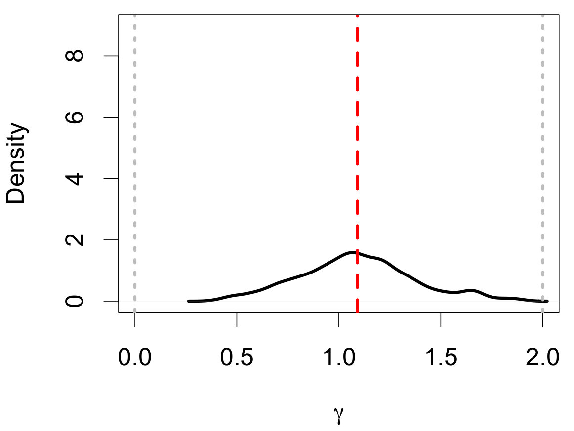 Figure 16
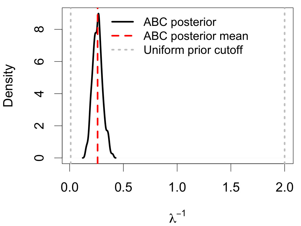 Figure 17
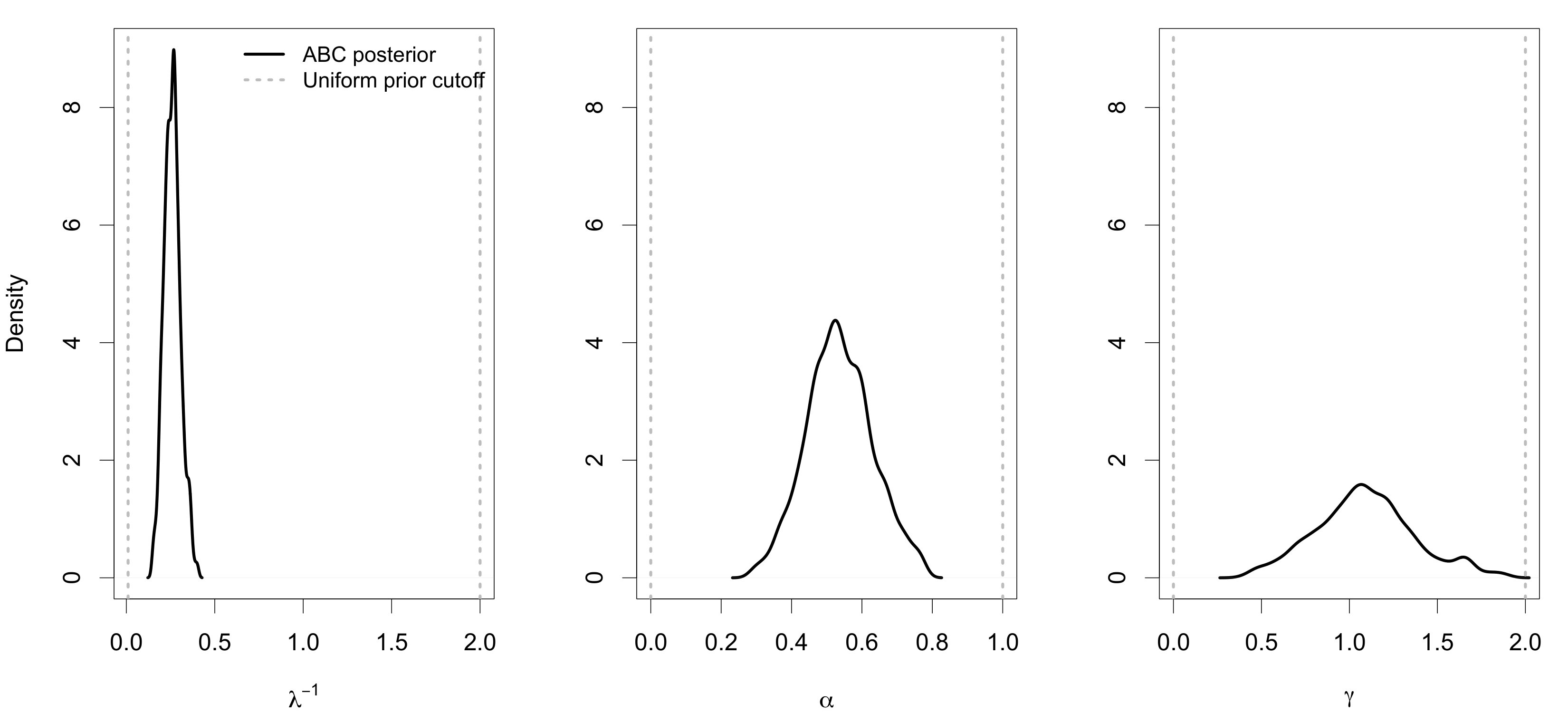 Figure 18
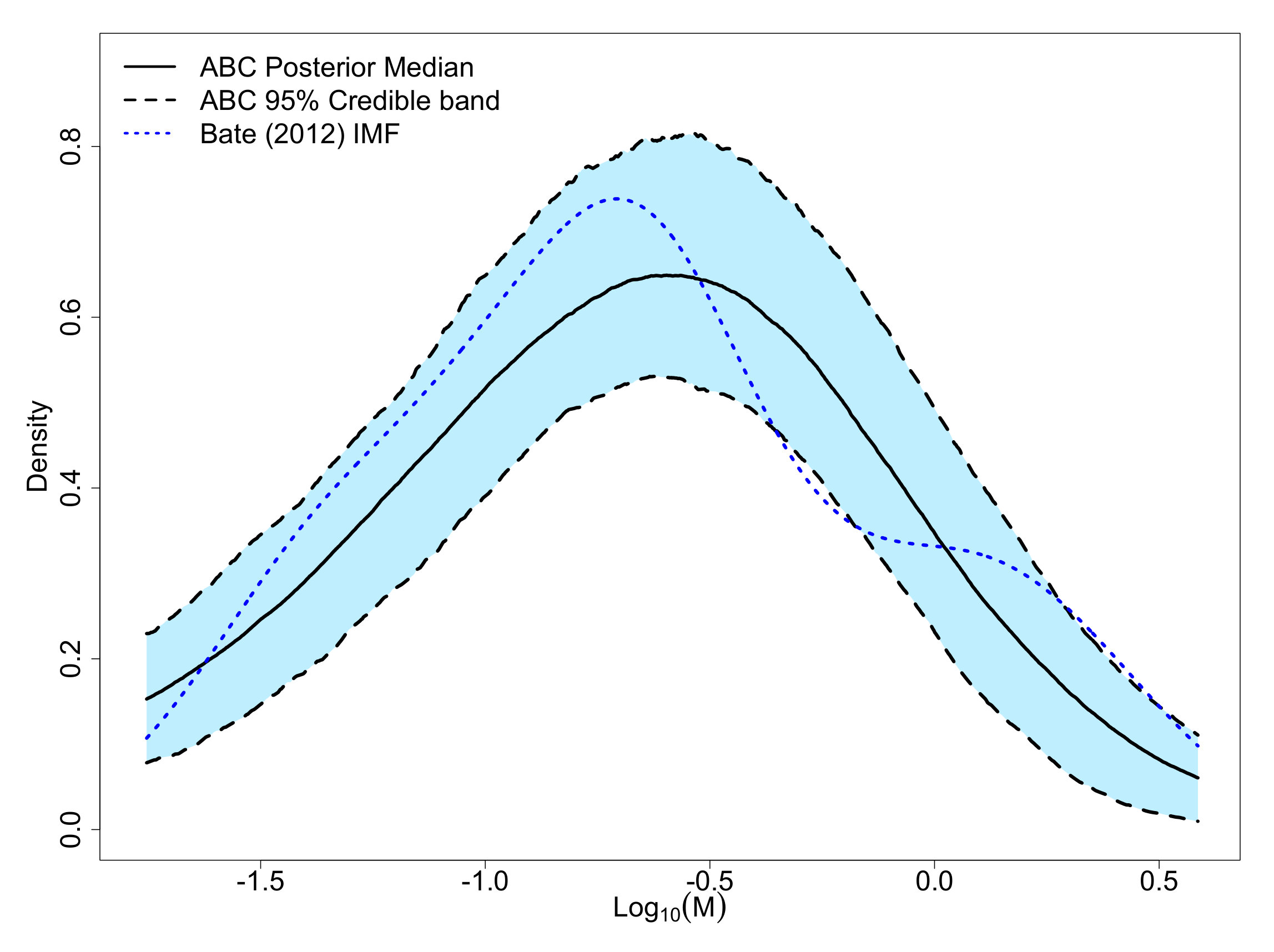 Figure 19
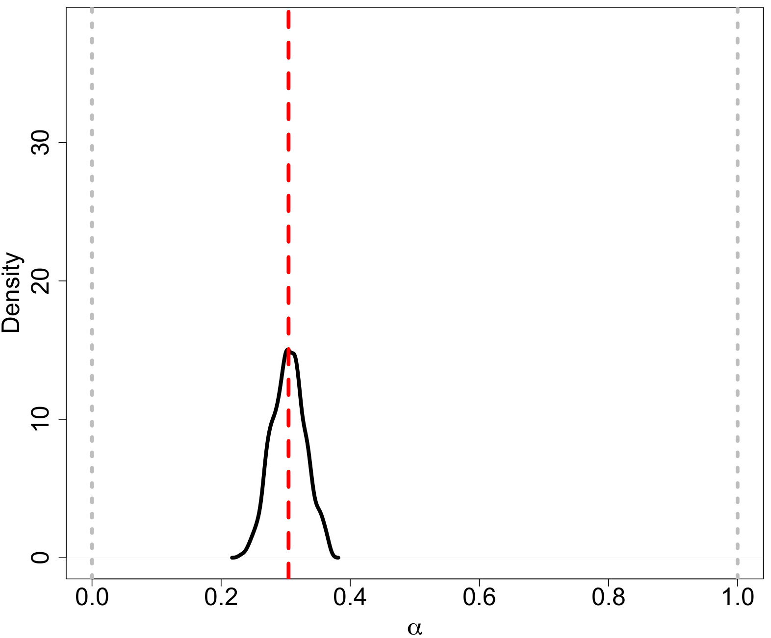 Figure 20
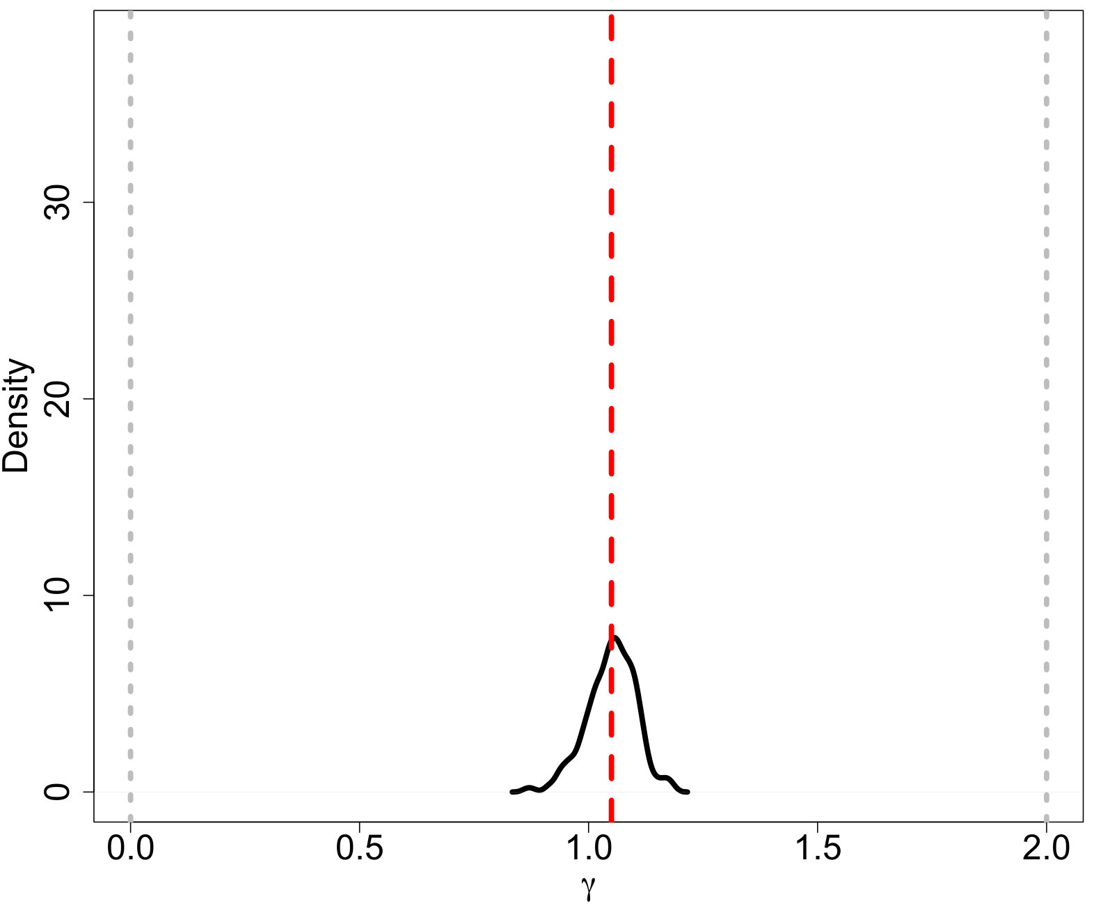 Figure 21
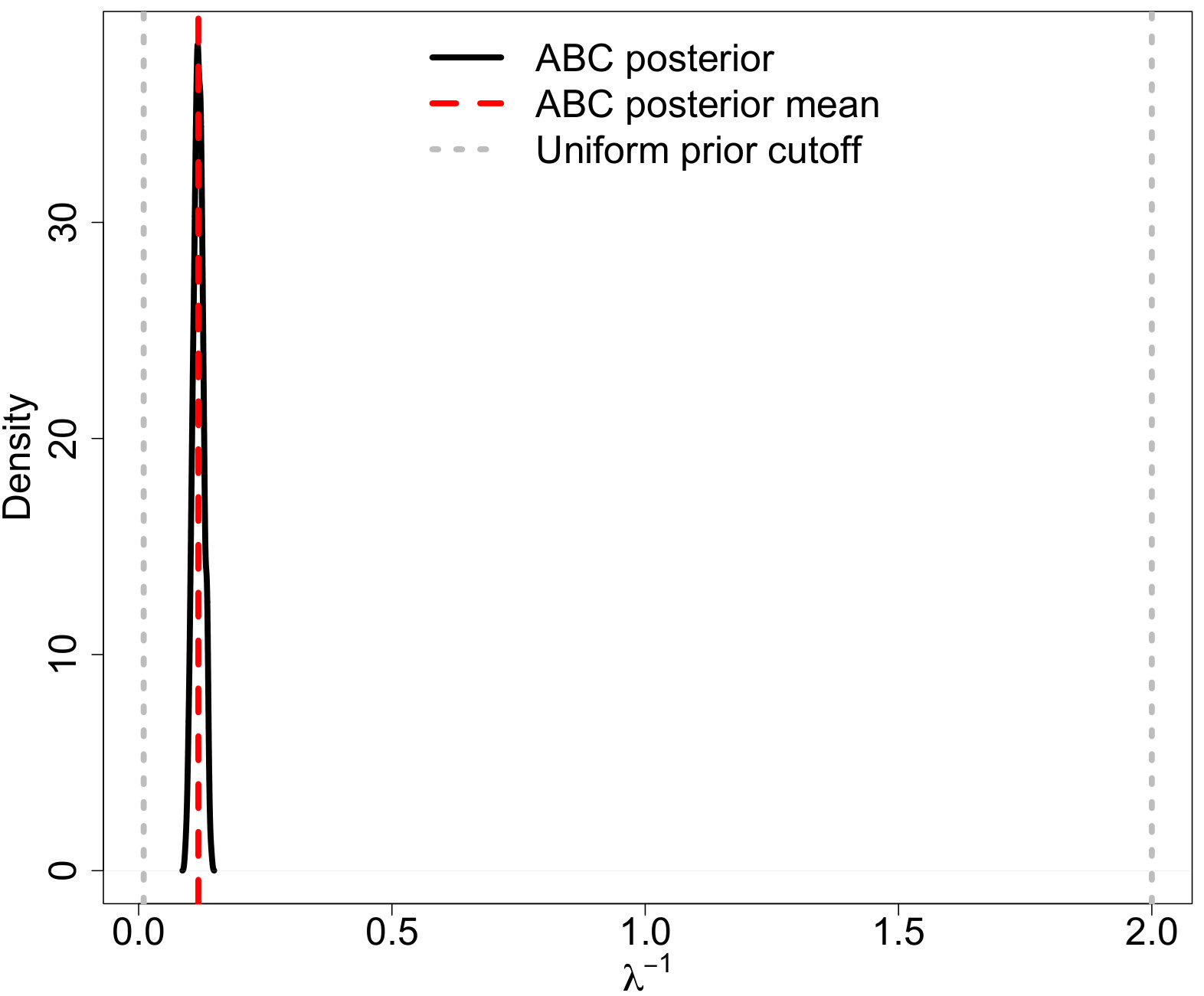 Figure 22
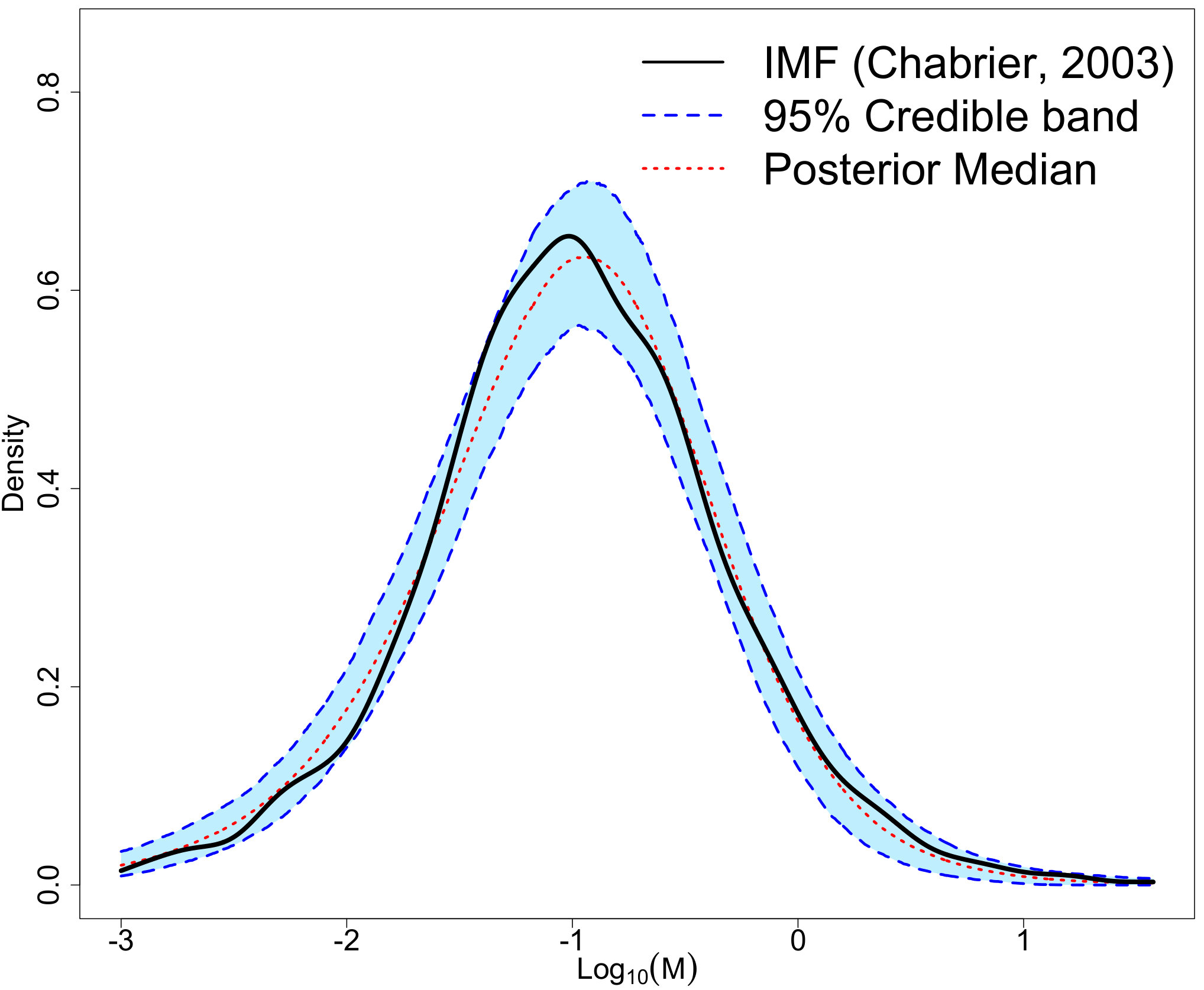 Figure 23
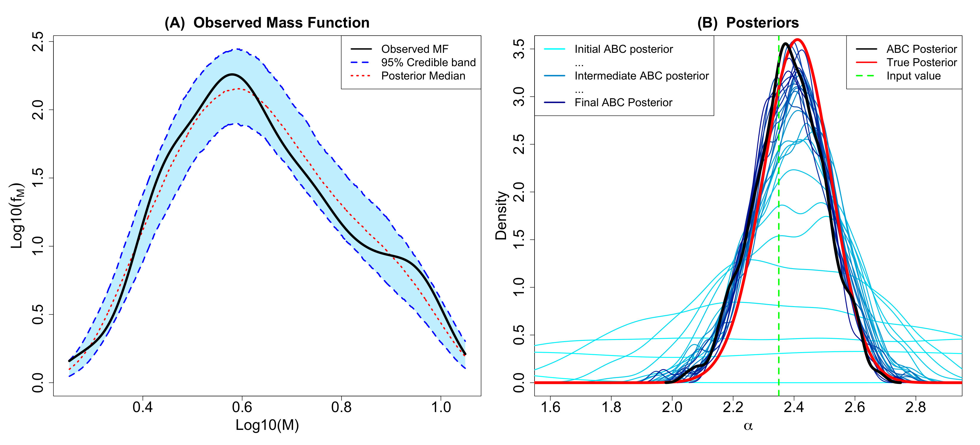 Figure 24
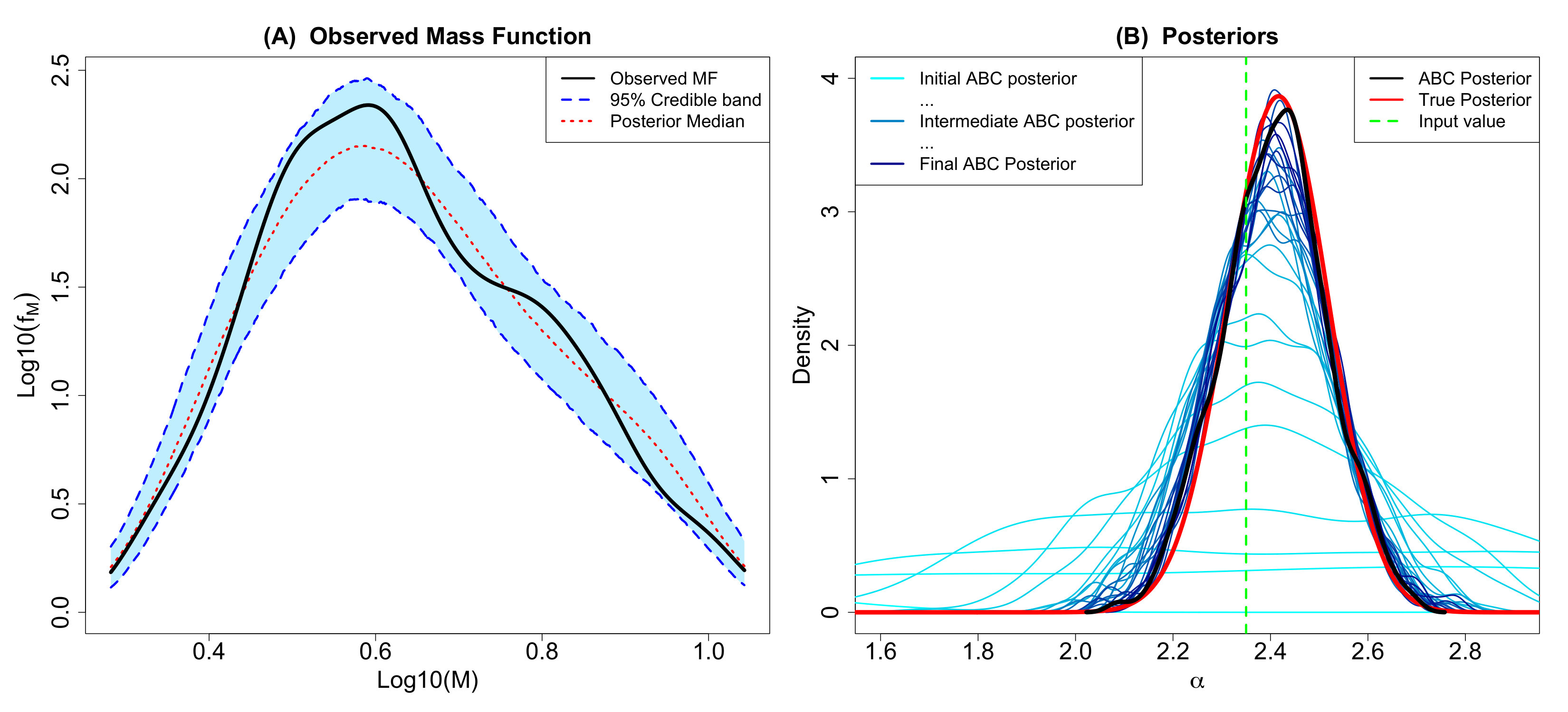 Figure 25
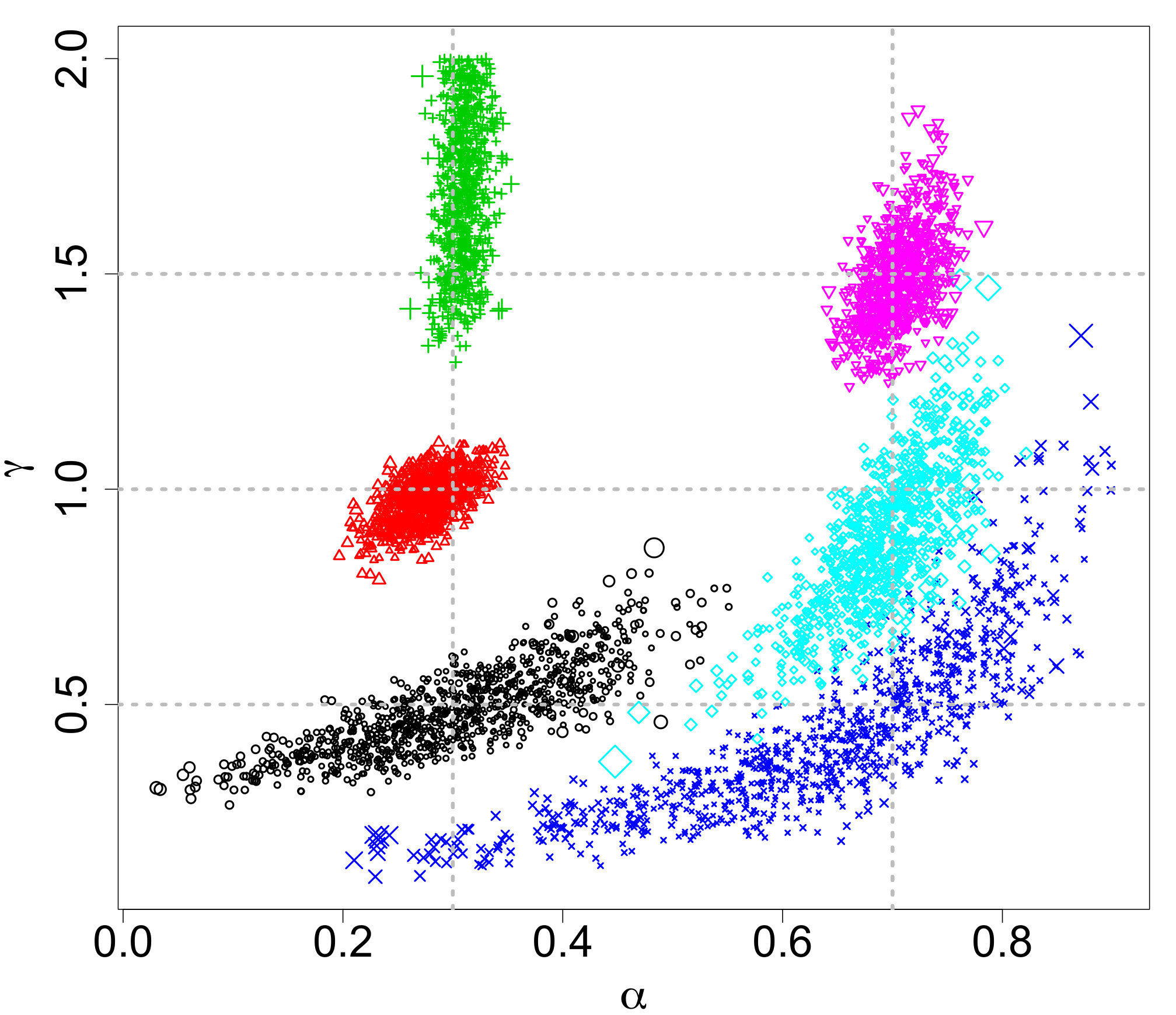 Figure 26
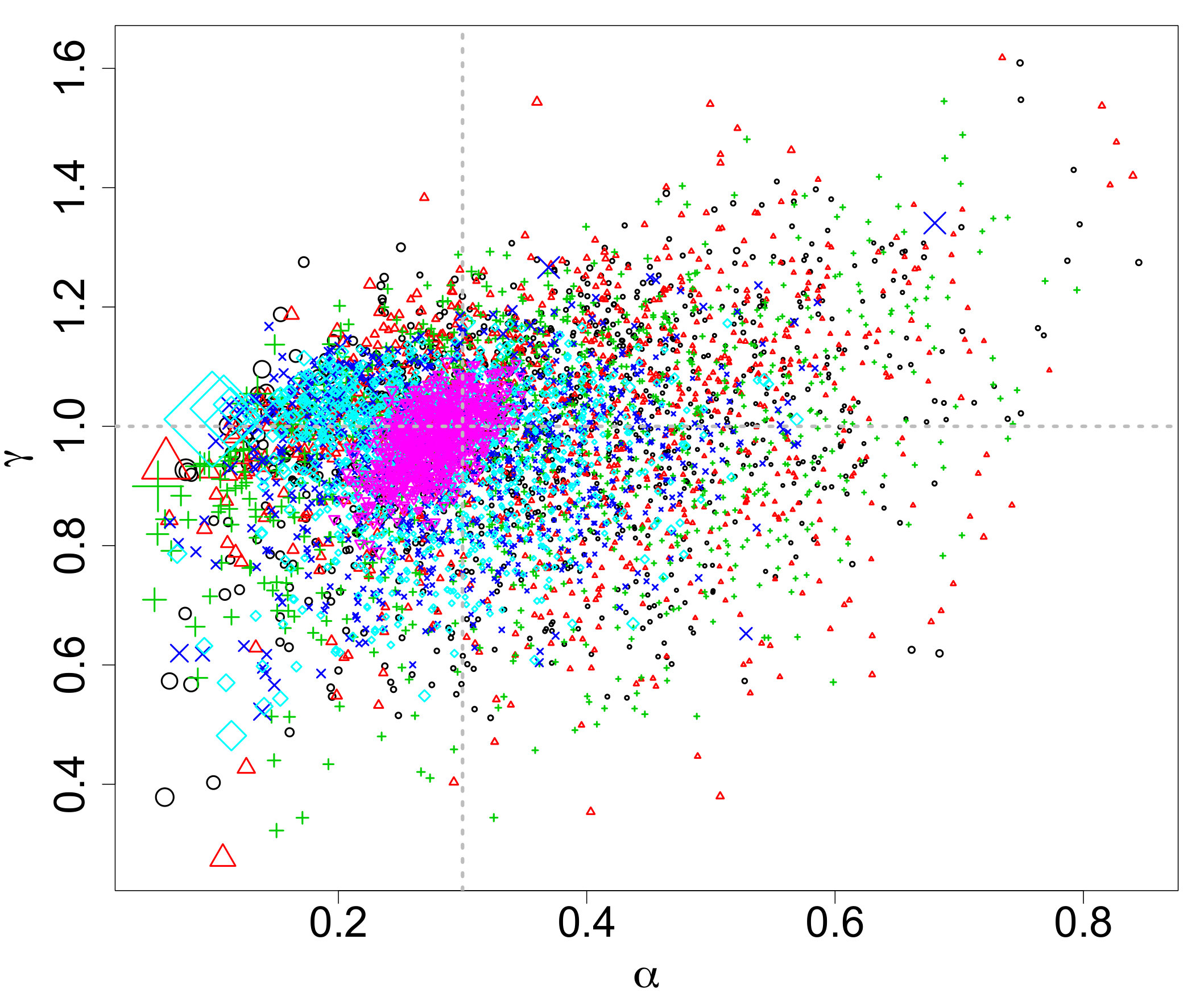 Figure 27
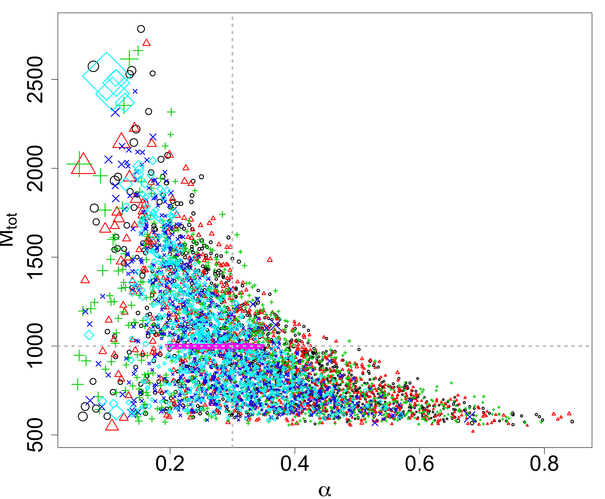 Figure 28
 Figure 29
 Figure 30
 Figure 31
 Figure 32
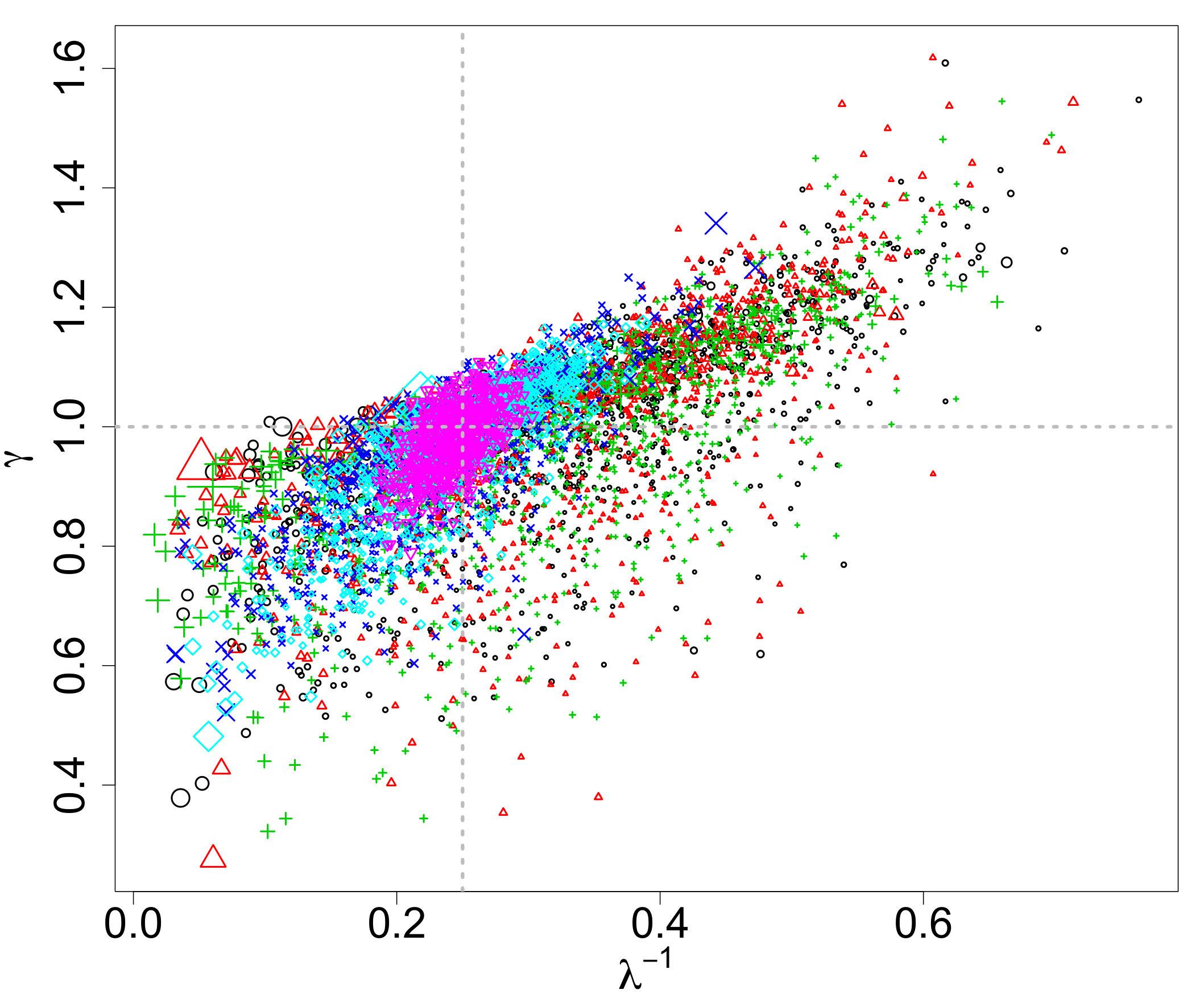 Figure 33
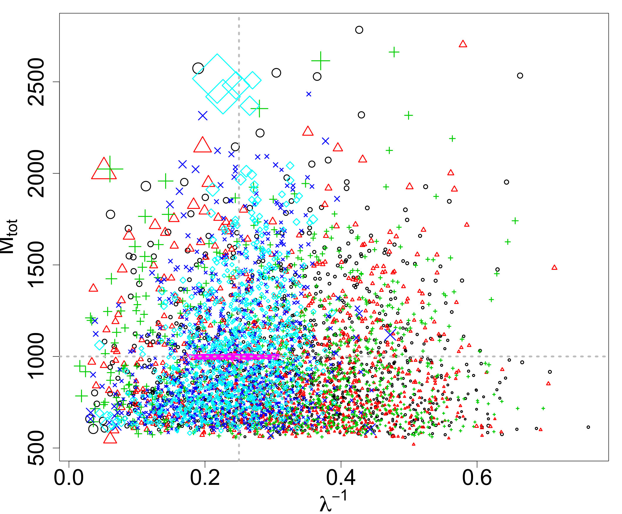 Figure 34
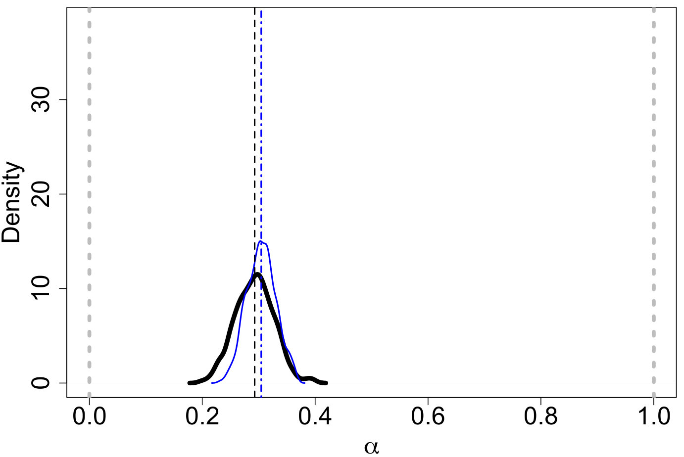 Figure 35
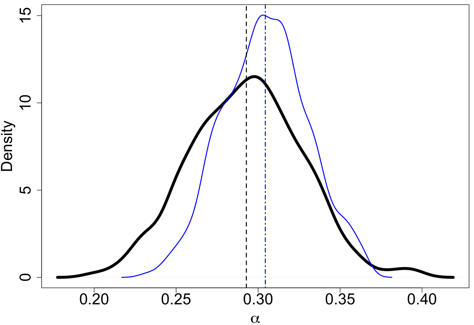 Figure 36
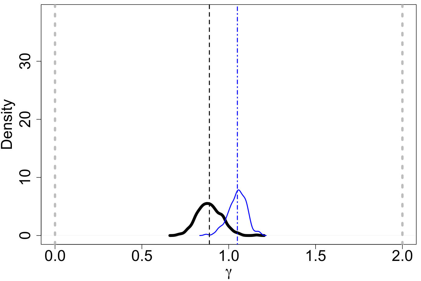 Figure 37
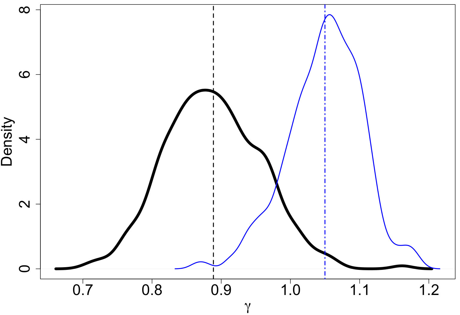 Figure 38
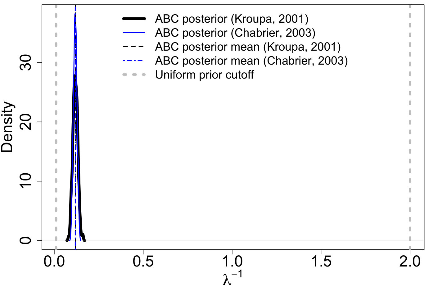 Figure 39
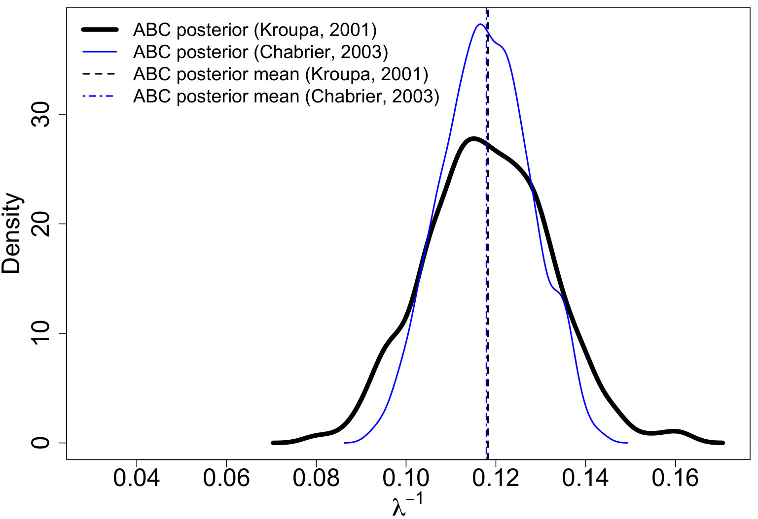 Figure 40
Peer Reviews
No public reviews on file for this paper yet. If you reviewed it on a platform where reviews are public (OpenReview, ICLR, NeurIPS, ICML), you can paste yours below so the community can read it here.
Code & Models
Videos
No videos yet. Explain this paper in a talk, walkthrough, or lecture? Add one.
A Preferential Attachment Model for the Stellar Initial Mass Function
Jessi Cisewski-Kehelabel=e1][email protected] [ Department of Statistics & Data Science
Yale University
New Haven, CT 06511
Grant Wellerlabel=e2][email protected] [ UnitedHealth Group Research & Development
Minneapolis, MN 55430
Chad Schafer label=e3][email protected] [ Department of Statistics & Data Science
Carnegie Mellon University
Pittsburgh, PA, 15213
Abstract
Accurate specification of a likelihood function is becoming increasingly difficult in many inference problems in astronomy. As sample sizes resulting from astronomical surveys continue to grow, deficiencies in the likelihood function lead to larger biases in key parameter estimates. These deficiencies result from the oversimplification of the physical processes that generated the data, and from the failure to account for observational limitations. Unfortunately, realistic models often do not yield an analytical form for the likelihood. The estimation of a stellar initial mass function (IMF) is an important example. The stellar IMF is the mass distribution of stars initially formed in a given cluster of stars, a population which is not directly observable due to stellar evolution and other disruptions and observational limitations of the cluster. There are several difficulties with specifying a likelihood in this setting since the physical processes and observational challenges result in measurable masses that cannot legitimately be considered independent draws from an IMF. This work improves inference of the IMF by using an approximate Bayesian computation approach that both accounts for observational and astrophysical effects and incorporates a physically-motivated model for star cluster formation. The methodology is illustrated via a simulation study, demonstrating that the proposed approach can recover the true posterior in realistic situations, and applied to observations from astrophysical simulation data.
The published version of this manuscript is available at https://doi.org/10.1214/19-EJS1556.
Approximate Bayesian computation,
astrostatistics,
computational statistics,
dependent data,
keywords:
\startlocaldefs\endlocaldefs
Contents
1 Introduction
The Milky Way is home to billions of stars (McMillan, 2016), many of which are members of stellar clusters - gravitationally bound collections of stars. Stellar clusters are formed from low temperature and high density clouds of gas and dust called molecular clouds, though there is uncertainty as to how the stars in a cluster form (Beccari et al., 2017). Each theory of star formation yields a different prediction for the distribution of the masses of stars that initially formed in a cluster. Hence, it is of fundamental interest to estimate this distribution, referred to as the stellar initial mass function (IMF), and assess the validity of these competing theories. The IMF can be thought of as a continuous density describing the distribution of star masses that initially form in a stellar cluster. In fact, research advances in many areas of stellar, galactic, and extragalactic astronomy are at least somewhat reliant upon accurate understanding of the IMF (Bastian, Covey and Meyer, 2010). For example, the IMF is a key component of galaxy and stellar evolution and planet formation (Bally and Reipurth, 2005; Bastian, Covey and Meyer, 2010; Shetty and Cappellari, 2014), along with chemical enrichment and abundance of core-collapse supernovae (Weisz et al., 2013).
There is also ongoing discussion surrounding the universality of the IMF, i.e., if a single IMF describes the generative distribution of stellar masses for all star clusters (Bastian, Covey and Meyer, 2010). The consensus of the astronomical community is that the IMF is not universal, however, most of the observations had been consistent with universality (Kroupa, 2001; Bastian, Covey and Meyer, 2010; Ashworth et al., 2017). With further research and growing sample sizes, however, there is increased theoretical (e.g., Bonnell, Clarke and Bate 2006; Dib et al. 2010) and observational (e.g., Treu et al. 2010; van Dokkum and Conroy 2010; Spiniello et al. 2014; Geha et al. 2013; Dib, Schmeja and Hony 2017) support for an IMF that can vary cluster to cluster.
Salpeter (1955) studied the evolutionary properties of certain populations of stars, and in the process defined the first IMF (which he called the “original mass function”). This work put forth the now-classic model for the IMF, a power law with a finite upper bound equal to the physical maximum mass of a star that could form in a cluster (Salpeter, 1955). More recent studies continue to use this power law form for the IMF, especially for stars of mass greater than half that of our sun (e.g., Massey 2003; Bastian, Covey and Meyer 2010; Da Rio et al. 2012; Lim et al. 2013; Weisz et al. 2013, 2015; Jose et al. 2017). Similar models have been proposed and used in the astronomical literature for inference of the stellar IMF; these will be discussed in the next section. The estimation of the parameters of these proposed models typically relies on the assumption that the observed stars in a stellar cluster form independently; more specifically, the assumption that the masses of the individual stars form independently. The proposed model in this work loosens the assumption of independence in order to explore one of several possible physical formation mechanisms of cluster formation and avoids specification of a parametric model form by using on a new simulation model.
Despite this seemingly simple form of the power law model, the statistical challenges of estimating the IMF using observed stars from a cluster are significant. Many of the limitations are related both to observational issues and to the adequate modeling of the evolution of a star cluster after the initial formation. For example, since stars of greater mass die more rapidly, the upper tail of the IMF is not observed in a cluster of sufficient age. Also, the death of massive stars can trigger additional star formation, contaminating the lower end of the IMF with new stars (Woosley and Heger, 2015). There are also issues related to missing lower-mass stars due to the sensitivity of the instruments. The observational astronomers will often estimate a completeness function of an observed cluster, which is the probability of observing a star of a particular mass. The completeness function is discussed in more detail below.
The observational limitations and the challenge of modeling cluster evolution make approximate Bayesian computation (ABC) appealing for estimation of the IMF, as ABC allows for relatively easy incorporation of such effects. The difficulty of addressing these limitations is implied by the fact that observational effects are often ignored or accounted for in an ad hoc or unspecified manner (e.g., Da Rio et al. 2012; Ashworth et al. 2017; Jose et al. 2017; Kalari et al. 2018), though Weisz et al. (2013) discuss how some observational limitations can be incorporated into their proposed Bayesian model. A primary appeal of ABC for this application is the ability to incorporate more complex models for cluster formation. Standard IMF models do not specify the process by which a large mass of gas (the molecular cloud) transforms into a gravitationally bound collection of stars. ABC is based on a simple rejection-sampling approach, in which draws of model parameters from a prior distribution are fed through a simulation model to generate a sample of data. If the generated sample is “close” (based on an appropriately chosen metric) to the observed data, the prior draw that produced that generated sample is retained. The collection of accepted parameter values comprise draws from an approximation to the posterior. The simulations (the forward model) can include any of the complex processes that make it challenging to derive a likelihood function for the observable data.
This situation is typical of inference challenges that arise in astronomy. See Schafer and Freeman (2012); Akeret et al. (2015); Ishida et al. (2015) for reviews. Recent years have seen a rapid increase in the use of ABC methods for estimation in this field, including specific application to Milky way properties (Robin et al., 2014), strong lensing of galaxies (Killedar et al., 2018; Birrer, Amara and Refregier, 2017), large scale structure of the Universe (Hahn et al., 2017), estimating the redshift distribution (Herbel et al., 2017), galaxy evolution (Hahn, Tinker and Wetzel, 2017), weak lensing (Peel et al., 2017; Lin and Kilbinger, 2015), exoplanets (Parker, 2015), galaxy morphology (Cameron and Pettitt, 2012), and supernovae (Weyant, Schafer and Wood-Vasey, 2013).
Hence, our motivation for using the proposed stochastic model for the stellar IMF includes both scientific and practical considerations. We model the observable data in a star cluster using a formation mechanism that incorporates realistic dependency in the masses of the stars. Further, this model generalizes commonly used IMF models, i.e., it can capture, but also distinguish, popular competing IMF model shapes. Flexible models of this type have great potential to test widely-held assumptions of more restrictive parametric forms, and eliminate the need for (often arbitrary) model selection exercises. Finally, the generative approach allows for the incorporation of observation effects and uncertainties within an ABC framework.
This paper is organized as follows. In Section 2, background on the IMF along with inference challenges are presented along with an introduction of ABC. The proposed stochastic model for stellar formation is discussed in Section 3. A simulation study, including an application of the proposed methodology to the estimation of the IMF of a realistic astrophysical simulation (Bate, 2012), can be found in Section 4. Finally, 5 provides a discussion.
2 Background
2.1 Stellar Initial Mass Function
As noted above, Salpeter (1955) introduced the power law model for the shape of the IMF for masses larger than 0.5, where is the mass of the Sun. Kroupa (2001) extended the range of the IMF by proposing a three-part broken power law model over the range , where is the mass of the largest star that could form with nonzero probability. This model postulates different forms for the IMF for stars of masses , and . To illustrate the form of the IMF model of Salpeter (1955), consider the upper tail where , and define then the probability density function for mass in the upper tail of the stellar IMF is assumed to be given by
[TABLE]
where the constant is chosen such that is a valid probability density. (For the form of the IMF model of Kroupa (2001), see Equation (3.2).) Alternative models have been proposed that include log-normal distributions, joint power law and log-normal parts, and truncated exponential distributions (Chabrier, 2003a, b, 2005; Corebelli, Palla and Zinnecker, 2005; Bastian, Covey and Meyer, 2010; Offner et al., 2014). The Kroupa (2001) and Chabrier (2003a, b) models are displayed in Figure 1 along with observational challenges discussed §2.1.1. Power law distributions and log-normal distributions are closely related and may be the result of subtle differences in the underlying formation mechanism (Mitzenmacher, 2004). The IMF model we propose will include, as a special case, a family of formation mechanisms that generate power law tails, but also allow for a wider range of tail behaviors (see Appendix A).
2.1.1 Observational Challenges
Observing all stars comprising an IMF is not feasible, as the most massive stars () have lifetimes of only a few million years. The lifetime of a star (the time it takes for the star to burn through its hydrogen) depends strongly on its mass: the most massive stars have shorter lives due to the hotter temperatures they must maintain to avoid collapse from the strong gravitational forces. In particular, stellar life is approximately proportional to where (Hansen, Kawaler and Trimble 2004, p. 30, Chaisson and McMillan 2011, p. 439). Hence, the mass of the largest star observed in a given cluster depends on the cluster age.
Furthermore, the IMF is estimated using a noisy, incomplete view of that cluster. Whether or not a star is observed is dependent on several factors including its mass, its location in the cluster, and its neighbors. Some of these factors are described by a data set’s completeness function, which quantifies a given star’s probability of being observed. This depends on its luminosity (i.e. intrinsic brightness) since it needs to be sufficiently bright to be observable; in particular, completeness depends on stellar flux in comparison with the flux limits of the observations. There are also issues with mass segregation: stars with lower mass tend to be on the edge of the cluster, while the most massive stars are often found in the center (Weisz et al., 2013). Due to stellar crowding in the center, stars in this region can be more difficult to observe. Additionally, binary stars (star systems consisting of a pair of stars) are difficult to distinguish from a single star, creating the potential for overstating the mass of an object and understating the number of stars in the cluster.
There are additional uncertainties involved in translating the actual observables (e.g. photometric magnitudes) into a mass measurement; that is, the mass values for observable stars are only estimates. The Hertzsprung-Russell (H-R) Diagram is a classic visual summary of the distribution of the luminosity and temperature of a collection of stars. A typical H-R Diagram includes a main sequence of stars that trace a line from bright and hot stars to dim and cool stars. Stellar mass also evolves along this one-dimensional feature, and since luminosity and temperature are estimable, mass can thus also be estimated. The mass of binary stars can be determined via Kepler’s Laws, and hence a mass-luminosity relationship can be fit to binaries and then extended to other stars on the main sequence. Unfortunately, luminosity and temperature are nontrivial to estimate, as corrections for effects such as accretion and extinction are required, along with an accurate estimate of the distance to the stars (Da Rio et al., 2010). The process is further complicated by the dependence of how these transformations are made on the spectral type of the star. Careful budgeting of the errors that accumulate is required in order to produce a reasonable error bars on mass estimates; Da Rio et al. (2010) utilize a Monte Carlo approach in which the errors in magnitudes are propagated forward through to uncertainties in the spectral type, the accretion and reddening corrections, and finally to an uncertainty on the mass.
2.2 Approximate Bayesian Computation
Standard approaches to Bayesian inference, either analytical or built on MCMC, require the specification of a likelihood function, , with data , and parameter(s) . In many modern scientific inference problems, such as for some emerging models for the stellar IMF, the likelihood is too complicated to be derived or otherwise specified. As noted previously, ABC provides an approximation to the posterior without specifying a likelihood function, and instead relies on forward simulation of the data generating process.
The basic algorithm for sampling from the ABC posterior is attributed to Tavaré et al. (1997) and Pritchard, Seielstad and Perez-Lezaun (1999), used for applications to population genetics. The algorithm has three main steps which are repeated until a sufficiently large sample is generated: Step 1, Sample from the prior; Step 2, Generate from the forward process assuming ; Step 3, Accept if , where is a user-specified distance function and is a tuning parameter that should be close to 0. This last step typically consists of comparing low-dimensional summary statistics generated for the observed and simulated datasets. Adequate statistical and computational performance of ABC algorithms depends greatly on the selection of such summary statistics (Joyce and Marjoram, 2008; Blum and François, 2010; Blum, 2010; Fearnhead and Prangle, 2012; Blum et al., 2013).
The basic ABC algorithm can be inefficient in cases where the parameter space is of moderate or high dimension. Hence, important adaptations of the basic ABC algorithm incorporate ideas of sequential sampling in order to improve the sampling efficiency (Marjoram et al., 2003; Sisson, Fan and Tanaka, 2007; Beaumont et al., 2009; Del Moral, Doucet and Jasra, 2011). A nice overview of ABC can be found in Marin et al. (2012). Here, we use a sequence of decreasing tolerances with the tolerance shrinking until further reductions do not significantly affect the resulting ABC posterior. The improvement in efficiency is due to the modification that happens after the first time step: instead of sampling from the prior distribution, the proposed are drawn from the previous time step’s ABC posterior. Using this adaptive proposal distribution can help to improve the sampling efficiency. The resulting draws, however, are not targeting the correct posterior, and so importance weights, , are used to correct this discrepancy.
3 Forward Model for the IMF
Due to their simple interpretations, mathematical ease, and demonstrated consistency with observations, power law IMFs (or similar variants) have been widely adopted in the astronomy literature (Kroupa et al., 2012); however, open questions remain about stellar formation processes. The proposed forward model is a way to link a possible stellar formation process with the realized mass function (MF).
One known underlying mechanism for producing data with power-law tails is based on preferential attachment (PA) (Mitzenmacher, 2004). The earliest PA model, the Yule-Simon process, was popularized by Simon (1955), and was originally used to model biological genera and word frequencies. Other PA models include the classic Chinese restaurant process and its generalizations (Bloem-Reddy and Orbanz, 2017). Interest in PA models grew within the study network evolution (Barabási and Albert, 1999). Such evolution is described by the attachment function, which describes the probability that a node acquires an additional edge, usually as an increasing function of its current degree. Most of the work done on estimation of the attachment function makes the assumption that observations are available regarding the full or partial evolution of the network. This includes the nonparametric methods of Jeong, Néda and Barabási (2003), Newman (2001), and Pham, Sheridan and Shimodaira (2015); the maximum likelihood approaches of Gómez, Kappen and Kaltenbrunner (2011), Wan et al. (2017a), Onodera and Sheridan (2014); and the Bayesian approach (using MCMC) taken by Sheridan, Yagahara and Shimodaira (2012). Wan et al. (2017a) also describes an approximation to the MLE that can be utilized when only a snapshot view of the network is available. Wan et al. (2017b) uses a semiparametric approach to fit to the upper tail of the network degree distribution. The focus is on how the estimator performs under deviations from the linear PA model and the “superstar” linear PA model, in which one node to which most of the other nodes attach. Estimation is based on extreme value theory. Kunegis, Blattner and Moser (2013) use a simple least squares method to estimate the exponent in a nonlinear, but parametric, PA model.
In what follows, the proposed data generating process will use ideas of PA to model the the evolution of a star cluster. The ABC approach will be well-suited to perform inference with this model, given its complexity and the available data.
3.1 Preferential attachment for the IMF
The formation of a star cluster is a complicated and turbulent process with different theories on the physical processes that lead to the origin of the stellar IMF (Chabrier, 2005; Bate, 2012; Offner et al., 2014; Pokhrel et al., 2018). It is generally understood that the molecular cloud fragments and then forms stellar cores with a distribution referred to as the core mass function (CMF). Whether evolution from the CMF to the IMF is random, deterministic, or something in between is debated (Offner et al., 2014). In the proposed work, we consider the case where star cores can increase in mass by accreting material from the surrounding cloud and a particular star’s final mass can be affected by its neighbors through turbulence or dynamical interactions. That is, rather than assuming that stellar masses in a cluster arise independently of each other, our PA model proposes a resource-limited mass accretion process between stellar cores whose ability to accumulate additional mass is a function of their existing masses. This dependence feature is particularly important for statistical inference, as models that assume independent observations of stellar masses are vulnerable to incorrect and misleading inference. Additionally, the mass of the largest star to form in a cluster is limited by the total cluster mass.
Our proposed stochastic model for stellar formation is as follows: we first fix a total available cluster mass . This quantity can be physically interpreted as the total mass available for stellar formation in a molecular cloud. At each time step , a random quantity of mass enters the collection of stars; becomes the mass of the first star. Subsequent masses entering the system form a new star with probability or join existing star with probability , defined as
[TABLE]
The generating process is complete when the total mass of formed stars first exceeds . The possible ranges of the three parameters are , , and .
For the growth component, the model allows for linear (), sublinear (), and superlinear () behavior; the limiting case of gives a uniform attachment model. Finally, the parameter acts as a scaling factor which controls the average ‘coarseness’ of masses joining the forming stellar cores.
The proposed PA mass generation model offers considerable flexibility to approximate existing IMF models in the literature. To illustrate the generality of the proposed model, IMF realizations were drawn assuming the Kroupa (2001) broken power-law model as the true model, defined as
[TABLE]
and the Chabrier (2003a, b) log-normal model, defined as
[TABLE]
where constants , , and are defined to make the densities continuous. Our proposed PA ABC procedure was then used for inference and Figure 2 displays the resulting posterior predictive IMFs. The proposed model captures the general shape of the true model. Figures 3(a) - 3(c) display ABC marginal posteriors for the broken power-law model of Kroupa (2001) and the log-normal model of Chabrier (2003a, b). Both the broken power-law and log-normal models have similar ABC posterior means for (0.293 and 0.304, respectively). However, the ABC posterior means for are notably different. The broken power-law model has an ABC posterior mean of 0.889 while the estimate for the log-normal model is 1.050. Since the Kroupa (2001) and Chabrier (2003a, b) models use the same power-law slope for masses greater than 0.5 and 1 , respectively, this suggests that the differences in are due to differences in the shape of the lower-mass end of the IMF. The proposed model offers an approach for discriminating these models.
3.2 Initial Mass Function to the Observed Mass Function
The PA model describes the formation of a star cluster at initial formation. In practice, we are not generally able to observe the star cluster after the initial formation because significant time is likely to have passed. When observation of a cluster occurs, the initial cluster will have changed due to aging and dynamical evolution of the cluster. Additionally, even if observation of the initial cluster was possible, there are observational and measurement uncertainties that would limit our capacity to get a perfect representation of the initial cluster. The actual observed cluster is referred to as the present-day observed MF, which describes the observed distribution of the stellar masses of a particular cluster.
Observation limitations can be easily incorporated into the ABC framework. For simplicity, we adopt a “linear ramp” completeness function describing the probability of observing a star of mass :
[TABLE]
We assume that the values and are known, though we note that selecting an appropriate completeness function is a difficult process which requires quantification from the observational astronomers for each set of data. Different models for the completeness function could also be considered, including those which allow for spatially-varying observational completeness. A benefit of ABC is the ease at which a new completeness function can be incorporated – it amounts to a simple change in the forward model.
Due to measurement error and practical limitations in translating luminosities into masses, the masses of stars are not perfectly known. This uncertainty can be incorporated in different ways; following Weisz et al. (2013), we assume that the inferred mass of a star is related to its true mass via
[TABLE]
where is a standard normal random variable, and is known measurement error. The model for mass uncertainties in (3.5) is simple and could be extended to account for other sources of uncertainty (e.g. redshift).
As noted previously, the lifecycle of a star depends on certain characteristics such as mass. In the proposed algorithm, stars generated in a cluster are aged using a simple truncation of the largest masses. That is, the distribution of stellar masses for a star cluster of age Myr is given by
[TABLE]
corresponding to stellar lifetimes of (10) Myr, where is the mass of the star (Hansen, Kawaler and Trimble, 2004; Chaisson and McMillan, 2011), and represents some specified IMF model. More sophisticated models that account for effects such as binary stars and stellar wind mass loss can be inserted into this framework.
4 Simulation study
We propose an ABC framework to make inferences on the IMF given a cluster’s present-day observed MF.111Code for running the proposed ABC-IMF algorithm is available at https://github.com/JessiCisewskiKehe/ABC_for_StellarIMF. Details about the proposed ABC method, including the algorithm, are presented in Appendix B. In this section we first consider a simulation study where the data are generated from the proposed forward model with observational effects, and then we consider data from an astrophysical simulation (Bate, 2012, 2014).
4.1 Simulated data with observational effects
We first consider a suite of simulations which incorporate aging, completeness, and measurement error, in order to analyze these effects on the resulting inference on the IMF. The same IMF was used throughout the simulations, with , , , and , but we vary the range of the linear ramp completeness function of Equation (3.4); is fixed at 0.08 and where low values of result in fewer stars removed from the IMF and, hence, a larger number of stars in the MF. All five sets of MFs are aged 30 Myr and have log-normal measurement error with . The observational effects, including the differing completeness function upper bounds, resulted in MF’s with 800 (70.1% of IMF stars), 659 (57.7%), 488 (42.7%), 415 (36.3%), and 352 (30.8%) stars for , respectively, compared to the original IMF with 1142 stars.
We are interested in the differences among the ABC posteriors and predictive IMFs among the varying values. The marginal ABC posteriors are displayed in Figure 4, which also includes the analogous ABC marginal posteriors without observational effects . Except for the marginal posteriors of , for , the posteriors get broader, which is expected because larger results in fewer observations and greater uncertainty. However, the marginal posteriors for , and are quite similar. The marginal posteriors of in Figure 4(d) are all similar and significantly broader than the case without observational effects. Hence, the observational effects appear to have a profound impact on inference for . The pairwise joint ABC posteriors are displayed in Figure 5 as a reference, and seem to follow the same general patterns noted for the marginals (i.e., they are broader as increases).
Finally, the posterior predictive IMFs are combined into a single plot displayed in Figure 6. As in the previous section, the posterior predictive IMFs are the pointwise medians of 1000 independent draws from the ABC posteriors of Figure 4. Also included in the figures are 95% credible bands based on the 2.5 and 97.5 percentiles of the 1000 posterior draws. The true IMF is plotted as a thick yellow line and the corresponding ABC posterior predictive IMF without observational effects is also displayed. The posterior predictive IMFs for and overlap well with the true IMF and the posterior predictive IMF without observational effects, but with wider 95% credible bands. The posterior predictive IMFs for and have similar shapes and 95% credible bands. Their posterior predictive IMFs peak at a higher mass than the others. These differences are not surprising given that there are far fewer stars below, for example, : 46, 61, and 96 stars for compared to 225 and 368 stars for , respectively, and 685 stars in that range for the original IMF.
The conclusion drawn from these simulations is that the completeness function affects the resulting inference – when more stars are missing from the original IMF due to the completeness function, the resulting ABC posteriors tend to be broader to reflect the increased uncertainty.
4.2 Astrophysical simulation data
Next we consider a star cluster generated from the radiation hydrodynamical simulation presented in Bate (2012) and published in Bate (2014).222The astrophysical data is available at https://ore.exeter.ac.uk/repository/handle/10871/14881 This simulation resulted in 183 stars and brown dwarfs with a total mass of the resulting objects of about 88.68 formed from a 500 molecular cloud of uniform density. Understanding that simulations are only an approximation of reality, this astrophysical simulation was implemented to include realistic physics of star cluster formation such as radiative feedback. The technical details of the simulation are beyond the scope of this work, but can be found in Bate (2012). Figure 7 displays the resulting IMF as a density and histogram.
In Bate (2012), validation of the simulated cluster was carried out by comparing its IMF with the model of Chabrier (2005), and was not able to statistically differentiate them using a Kolmogorov-Smirnov test. The Chabrier (2005) IMF is displayed in Figure 7 as a comparison to the simulation data. While the general shape does appear to match well, the Bate (2012) data has a small second mode around . The Bate (2012) data seems to have more objects on the lower mass end and fewer between 0.5 and 1 than expected with the Chabrier (2005) IMF model. Additionally, because the shape of the low-mass end of the IMF is not well-constrained observationally, Bate (2012) compares the ratio of number of brown dwarfs to number of stars with masses and finds acceptable agreement with observations. Bate (2012) also carryout an analysis of the mechanism(s) behind the shape of the IMF. They found that larger objects have had longer accretion times, while lower mass objects tended to have a dynamical encounter that result in the accretion terminating; hence there ended up being, as Bate (2012) described, a “competition between accretion and dynamical encounters.” This competition for material seems consistent with the ideas underlying the proposed PA model.
The 183 objects were used as the observations in the proposed ABC algorithm using 1000 particles, 5 sequential time steps, a of (for adaptively initializing the algorithm), and the 25th percentile for shrinking the sequential tolerances based on the empirical distribution of the retained distances from the preceding time step. The resulting ABC marginal posteriors are displayed in Figure 8, the pairwise ABC joint posteriors in Figure 9, and the posterior predictive IMF in Figure 10. The ABC posterior means for , , and are 0.260, 0.537, and 1.091, respectively. The ABC posterior mean of is notably higher than the ABC posterior means of for the Kroupa (2001) (0.293) and Chabrier (2003a, b) (0.304) simulated data discussed in Section 3.1 (see Figure 2). The ABC posterior mean of is also slightly higher than the 1.050 posterior mean of the Chabrier (2003a, b) data. Though the IMF has a slightly irregular shape with a small second mode around 1 as noted previously, the proposed ABC method’s posterior predictive median and 95% predictive bands generally fit the IMF shape well.
5 Discussion
Accounting for the complex dependence structure in observable data, such as the initial masses of stars formed from a molecular cloud, is a challenging statistical modeling problem. A possible, but unsatisfactory, resolution is to proceed as though the dependency is sufficiently weak that an independence assumption is acceptable. Such approximations can be reasonable at small sample sizes, but are often revealed to be insufficient by modern data sets. Instead, we draw on PA models, proposing a new forward model for star formation. Though the new generative model was motivated by inference on stellar IMFs, the general concept is generalizable to other applications. Simulation-based approaches to inference, including ABC, allow for inference with such models.
The new generative model starts with the total mass of the system and stochastically builds individuals stars of particular mass at a sub-linear, linear, or super-linear rate. A goal of the proposed model and algorithm is to begin making a statistical connection between the observed stellar MF and the formation mechanism of the cluster, not that the proposed model shape is superior to the standard IMF models. Rather, the proposed model is more general in the sense that it captures the dependencies among the masses of the stars by connecting the star masses to a possible cluster formation mechanism, and also can accommodate standard models proposed in the astronomical literature. Additionally, by coupling the proposed model with ABC, observational limitations such as the aging and completeness of the observed cluster can easily be accounted for. Code for running the proposed ABC-IMF algorithm is available at https://github.com/JessiCisewskiKehe/ABC_for_StellarIMF.
In agreement with other studies that have implemented ABC algorithms (e.g. Weyant, Schafer and Wood-Vasey 2013; Ishida et al. 2015), we found the selection of informative summary statistics to be a crucial, but challenging step in the algorithm development. In the IMF setting, we had initially considered a number of different possible summary statistics, but it became clear that matching the shape of the IMF was important to constrain the parameters (along with the number of stars generated in the cluster). To assess the similarity between the observed and simulated IMFs, the distance was effective, but we imagine that other functional distances could also work well. In future applications of ABC, practitioners may find it useful to consider functional summaries and distances if the setting allows for it. To reach these conclusions, it required us to create a simplified setting where the true posterior was available; when possible, we suggest others consider this when trying to select useful summary statistics and distance functions.
While the proposed model is able to account for a particular dependency among the masses during cluster formation, there are several extensions that would be scientifically and statistically interesting. First, the generative model could be extended to capture the spatial dependency among the observations. Intuitively, such an approach could account for a mechanism that limits the formation of multiple very massive stars relatively near to each other. Understanding the spatial distribution of masses of stars during formation would help advance our understanding of stellar formation and evolution. Other effects that could be incorporated into the generative model include accounting for binary and other multiple star systems, the possible disturbances to the observed MF as stars die (beyond the censoring of the most massive stars), or spatial completeness functions (i.e. a completeness function that depends on not only the mass of the object, but also its location in the cluster).
Hence, the proposed generative model, used in conjunction with ABC, provides a useful framework for dealing with complex physical processes that are otherwise difficult to work with in a statistically rigorous fashion. As increasing computational resources allow for greater model complexity in astronomy and other fields, the proposed and other ABC algorithms may open new opportunities for Bayesian inference in challenging problems. There appears to be significant potential to extend this approach to even more complicated situations.
Appendix A Generating power law tails
As mentioned in Section 2, the PA model with linear evolution (the Yule-Simon Process) is known to generate power law tails (Newman, 2005). It is worth exploring the extent to which power law tail behavior is present in cases where , as the power law model is a prevalent assumption in this application, such as with the Kroupa (2001) and Chabrier (2003a, b) models. For example, it would be of interest to determine if tests of would have power to detect deviation from power law tails, which would be of interest to astronomers.
A small simulation study was conducted. Goodness-of-fit was assessed using the standard Kolmogorov-Smirnov statistic, with the empirical distribution of the masses of a collection of stars generated from our PA model compared to the best fitting power law model. As we are only interested in fitting to the upper tail, this analysis is restricted to the region above . We fix and , and consider , for values of ranging from 0.25 to 5. Fifty data sets are generated for each combination. Results are shown in Figure 11. In order to place the goodness-of-fit on a readily-interpretable scale, the p-value is calculated for each K-S test, and the median across the 50 repetitions is displayed. The results support the claim that the tail follows the power law when , but that the power law fit degrades quickly for outside . The effect is particularly strong for smaller values of . In practice, one may decide to use a prior distribution on that places more mass within if a power law model is expected, instead of the uniform prior distribution considered in this paper.
Appendix B Proposed ABC algorithm
The proposed ABC algorithm is displayed in Algorithm (1), where is the desired particle sample size to approximate the posterior distribution, and is motivated by the adaptive and sequential ABC algorithm of Beaumont et al. (2009). The forward model, , in Algorithm (1) is where the IMF masses are drawn and observational limitations and uncertainties, stellar evolution, and other astrophysical elements can be incorporated as outlined in Section 3. The other details of the proposed algorithm are discussed next.
Algorithm (1) is initialized using the basic ABC rejection algorithm at time step using a distance function to measure the distance between the simulated and observed datasets, and , respectively. The first tolerance, , is adaptively selected by drawing particles for some . Then the particles that have the smallest distance are retained, and is defined as the largest of those distances retained. For subsequent time steps (), rather than proposing a draw, , from the prior, , the proposed is selected from the previous time step’s () ABC posterior samples. The selected is then moved according to some kernel, , to ameliorate degeneracy as the sampler evolves. In order to ensure the true posterior (which requires sampling from the prior) is targeted, the retained draws are weighted according to the appropriate importance weights, – this incorporates the proposal distribution’s kernel.
A key step in the implementation of an ABC algorithm is to quantify the distance between the simulated and observed stellar masses. We define a bivariate summary statistic and distance function that captures the shape of the present-day MF and the random number of stars observed, displayed in Equations (B.1) and (B.2), respectively. For the shape of the present-day MF, we use a kernel density estimate of the masses (due to the heavy-tailed distribution of the initial masses), and an distance between the simulated and observed MF estimates. The number of stars observed is the other summary statistic, with the distance being the absolute value of the difference in the ratio of the counts from 1. More specifically, the bivariate summary statistic is defined as
[TABLE]
where the are kernel density estimates of , and and are the number of stars comprising the simulated and observed MF, respectively. These summary statistics were selected based on performance of a simulation study using the high-mass section of the broken power-law model because the true posterior is known in this setting. Results and additional discussion of the simulation study is presented below in Appendix B.1.
With the bivariate summary statistic, we use a bivariate tolerance sequence, , for is such that for . At time step , the tolerances are determined based on the empirical distribution of the retained distances from time step (e.g. the percentile). As noted previously, the tolerance sequence is initialized adaptively by selecting proposals from the prior distributions, then the proposals that result in the smallest distances were selected.333The sampled distances were scaled, squared, and then added together; the smallest of these combined distances were retained. The distance function and tolerance sequence displayed in Algorithm (1) are defined as , and (which can also be expanded to include the additional summary statistic noted below).
In practice, is an unknown quantity of interest. A prior can be assigned to and an additional summary statistic and tolerance sequence can be used. The summary statistic selected in this case is
[TABLE]
where and are the masses of the individual simulated and observed stars, respectively.
B.1 ABC summary statistic selection
In order to select effective summary statistics for the proposed model, we first employ the ABC methodology in a simplified study that focuses on the posterior of the power law parameter from Equation (2.1). We generate a cluster of stars from an IMF with slope (Salpeter, 1955), , and , and a uniform prior distribution for . This model was used in order to check the method against the true posterior of after the observational and aging effects have been incorporated into the forward model. We use the bivariate summary statistic and distance function of Equation (B.1) and (B.2). Defining the two-dimensional tolerance sequence as where the subscript indicates the algorithm time step, and and were selected using an adaptive start as discussed above using an initial number of draws of with . The algorithm ran for time steps. At steps , and were set equal to the percentile of the distances retained at the previous step from their corresponding distance functions.
The pseudo-data were aged 30 Myr, log-normal measurement error with , and observation completeness defined by the linear-ramp function in (3.4) with and . The simulated IMF and resulting MF (after the noted observational effects were applied) are displayed in Figure 12. The IMF is the object of interest, while the MF contain the actual observations that can be used for analysis.
The ABC posterior resulting from the ABC algorithm along with the true posterior for are displayed in Figure 13(a). The ABC posterior matches the true posterior, defined as
[TABLE]
where is the upper-tail mass cutoff due to aging. The close match between the true and ABC posteriors suggests that the selected summary statistics are useful for carrying out the ABC analysis. Figures 13(b) and 13(c) display the ABC posterior predictive IMF and MF. Even in regions where stars are missing due to the observational limitations, the ABC predictive median is still able to recover the shape of the original IMF (though with wider credible bands).
Acknowledgements
The authors thank the Yale Center for Research Computing for the resources we used for producing this paper. The authors also thank two anonymous reviewers, along with David W. Hogg, and Ewan Cameron for their comments and feedback on this work. Jessi Cisewski-Kehe and Grant Weller were partially supported by the National Science Foundation under Grant DMS-1043903. Chad Schafer was supported by NSF Grant DMS-1106956. Any opinions, findings, and conclusions or recommendations expressed in this material are those of the authors and do not necessarily reflect the views of the National Science Foundation.
The reference list from the paper itself. Each links out to its DOI / PubMed record.
- 1Akeret et al. (2015) {barticle} [author] \bauthor \bsnm Akeret, \bfnm Joel \binits J., \bauthor \bsnm Refregier, \bfnm Alexandre \binits A., \bauthor \bsnm Amara, \bfnm Adam \binits A., \bauthor \bsnm Seehars, \bfnm Sebastian \binits S. and \bauthor \bsnm Hasner, \bfnm Caspar \binits C. ( \byear 2015). \btitle Approximate Bayesian Computation for Forward Modeling in Cosmology. \bjournal ar Xiv preprint ar Xiv:1504.07245. \endbibitem
- 2Ashworth et al. (2017) {barticle} [author] \bauthor \bsnm Ashworth, \bfnm G. \binits G., \bauthor \bsnm Fumagalli, \bfnm M. \binits M., \bauthor \bsnm Krumholz, \bfnm M. R. \binits M. R., \bauthor \bsnm Adamo, \bfnm A. \binits A., \bauthor \bsnm Calzetti, \bfnm D. \binits D., \bauthor \bsnm Chandar, \bfnm R. \binits R., \bauthor \bsnm Cignoni, \bfnm M. \binits M., \bauthor \bsnm Dale, \bfnm D. \binits D., \bauthor \bsnm Elmegreen, \bfnm B. G. \binits B. G., \bauthor \bsnm
- 3Bally and Reipurth (2005) {bbook} [author] \bauthor \bsnm Bally, \bfnm J. \binits J. and \bauthor \bsnm Reipurth, \bfnm B. \binits B. ( \byear 2005). \btitle The Birth of Stars and Planets. \bpublisher Cambridge University Press, \baddress New York. \endbibitem
- 4Barabási and Albert (1999) {barticle} [author] \bauthor \bsnm Barabási, \bfnm Albert-László \binits A.-L. and \bauthor \bsnm Albert, \bfnm Réka \binits R. ( \byear 1999). \btitle Emergence of Scaling in Random Networks. \bjournal Science \bvolume 286 \bpages 509–512. \bdoi 10.1126/science.286.5439.509 \endbibitem
- 5Bastian, Covey and Meyer (2010) {barticle} [author] \bauthor \bsnm Bastian, \bfnm Nate \binits N., \bauthor \bsnm Covey, \bfnm Kevin R \binits K. R. and \bauthor \bsnm Meyer, \bfnm Michael R \binits M. R. ( \byear 2010). \btitle A universal stellar initial mass function? A critical look at variations. \bjournal Annu. Rev. Astron. Astr. \bvolume 48 \bpages 339–389. \endbibitem
- 6Bate (2012) {barticle} [author] \bauthor \bsnm Bate, \bfnm Matthew R \binits M. R. ( \byear 2012). \btitle Stellar, brown dwarf and multiple star properties from a radiation hydrodynamical simulation of star cluster formation. \bjournal Monthly Notices of the Royal Astronomical Society \bvolume 419 \bpages 3115–3146. \endbibitem
- 7Bate (2014) {barticle} [author] \bauthor \bsnm Bate, \bfnm Matthew R \binits M. R. ( \byear 2014). \btitle The statistical properties of stars and their dependence on metallicity: the effects of opacity. \bjournal Monthly Notices of the Royal Astronomical Society \bvolume 442 \bpages 285–313. \endbibitem
- 8Beaumont et al. (2009) {barticle} [author] \bauthor \bsnm Beaumont, \bfnm Mark A \binits M. A., \bauthor \bsnm Cornuet, \bfnm Jean-Marie \binits J.-M., \bauthor \bsnm Marin, \bfnm Jean-Michel \binits J.-M. and \bauthor \bsnm Robert, \bfnm Christian P \binits C. P. ( \byear 2009). \btitle Adaptive approximate Bayesian computation. \bjournal Biometrika \bvolume 96 \bpages 983–990. \endbibitem
