Double Quantum Dot scenario for spin resonance in current noise
Baruch Horovitz, Anatoly Golub

TL;DR
This paper demonstrates that interference effects in double quantum dots with spin-orbit coupling and Coulomb interactions produce current noise resonances at Larmor frequencies, explaining observed spin resonance phenomena in STM noise.
Contribution
It introduces a double quantum dot model showing how interference and spin interactions cause measurable noise resonances, expanding understanding of spin resonance in quantum transport.
Findings
Resonances occur at Larmor frequencies due to interference in double quantum dots.
Resonance lines are comparable in strength to shot noise background.
The model explains spin resonance observations in STM noise with non-polarized leads.
Abstract
We show that interference between parallel currents through two quantum dots, in presence of spin orbit interactions and strong on-site Coulomb repulsion, leads to resonances in current noise at the corresponding Larmor frequencies. An additional resonance at the difference of Larmor frequencies is present even without spin-orbit interaction. The resonance lines have strength comparable to the background shot noise and therefore can account for the numerous observations of spin resonance in STM noise with non-polarized leads. We solve also several other models that show similar resonances.
Click any figure to enlarge with its caption.
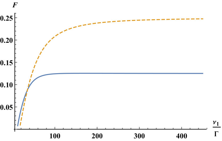 Figure 1
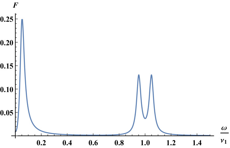 Figure 2
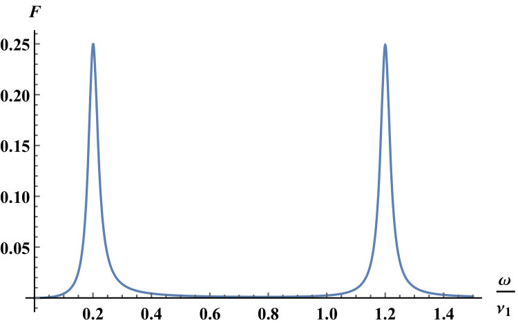 Figure 3
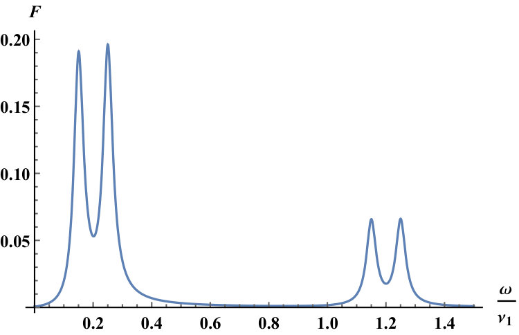 Figure 4
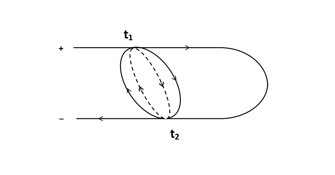 Figure 5
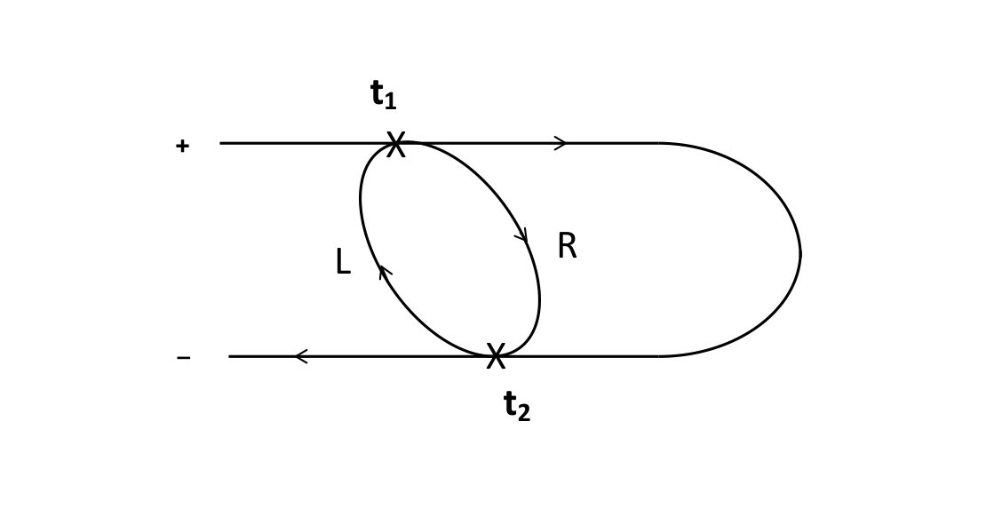 Figure 6
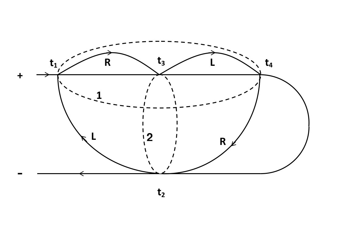 Figure 7
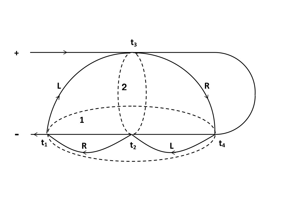 Figure 8
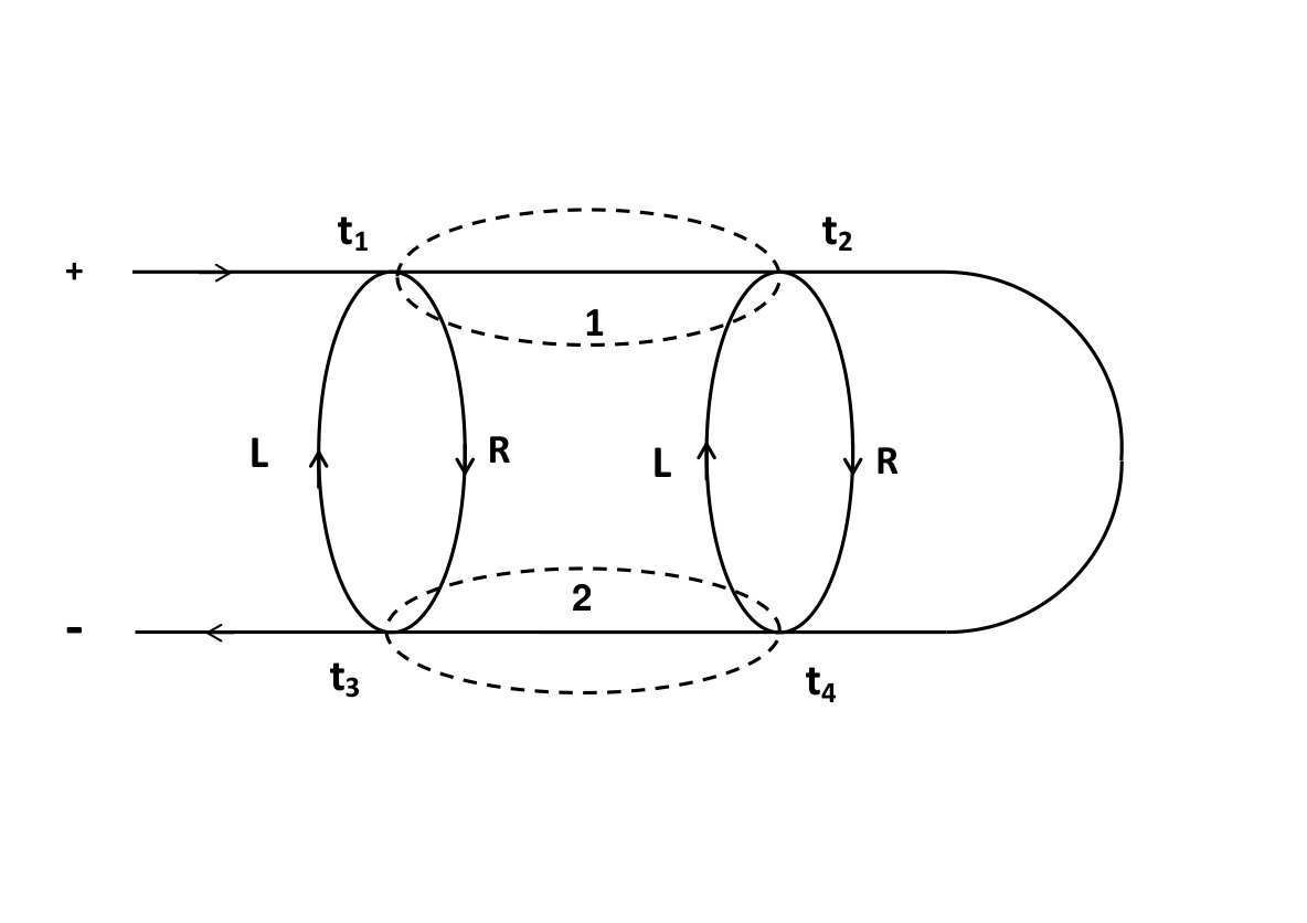 Figure 9
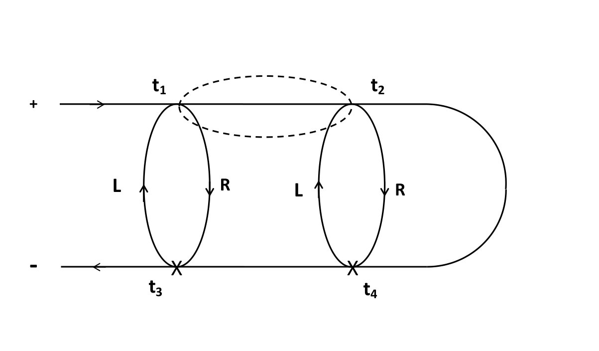 Figure 10
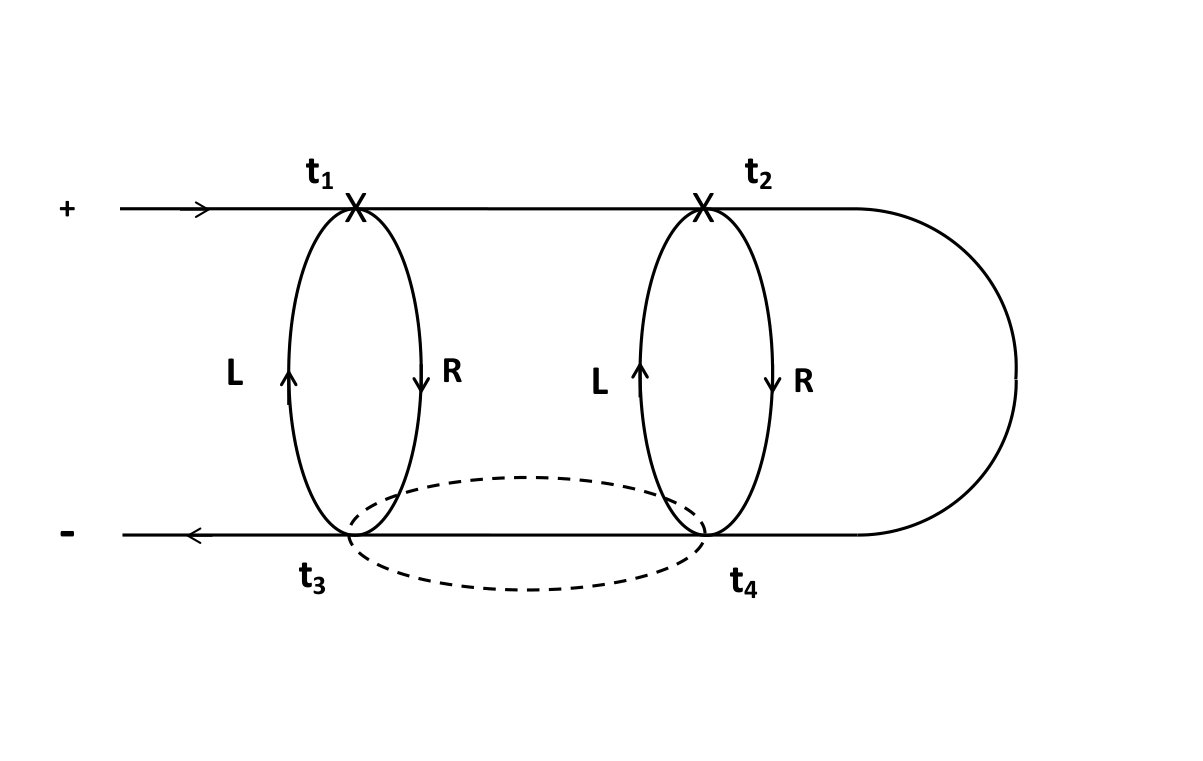 Figure 11
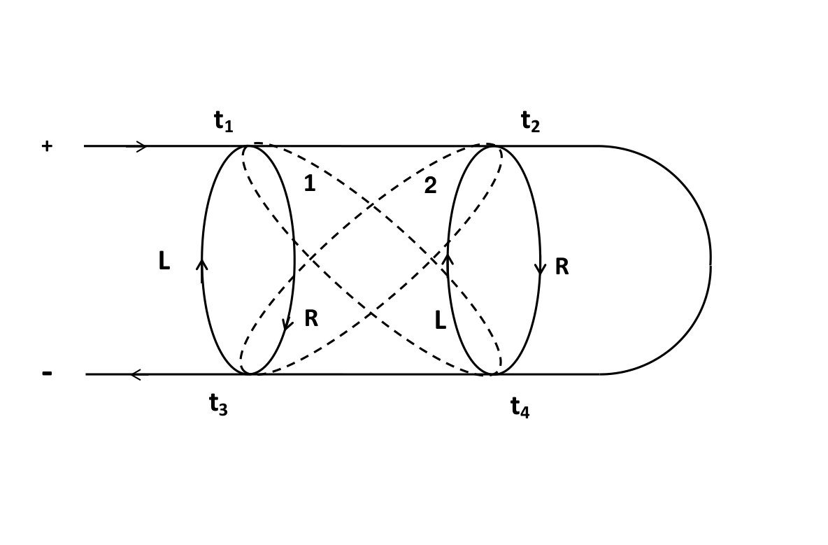 Figure 12
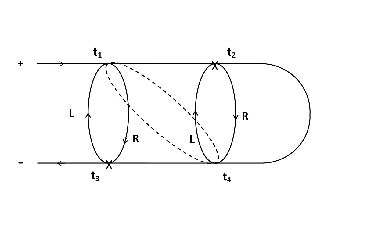 Figure 13
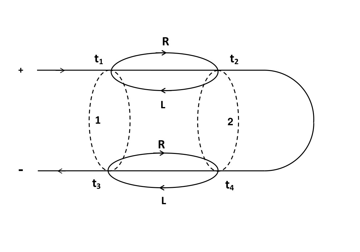 Figure 14
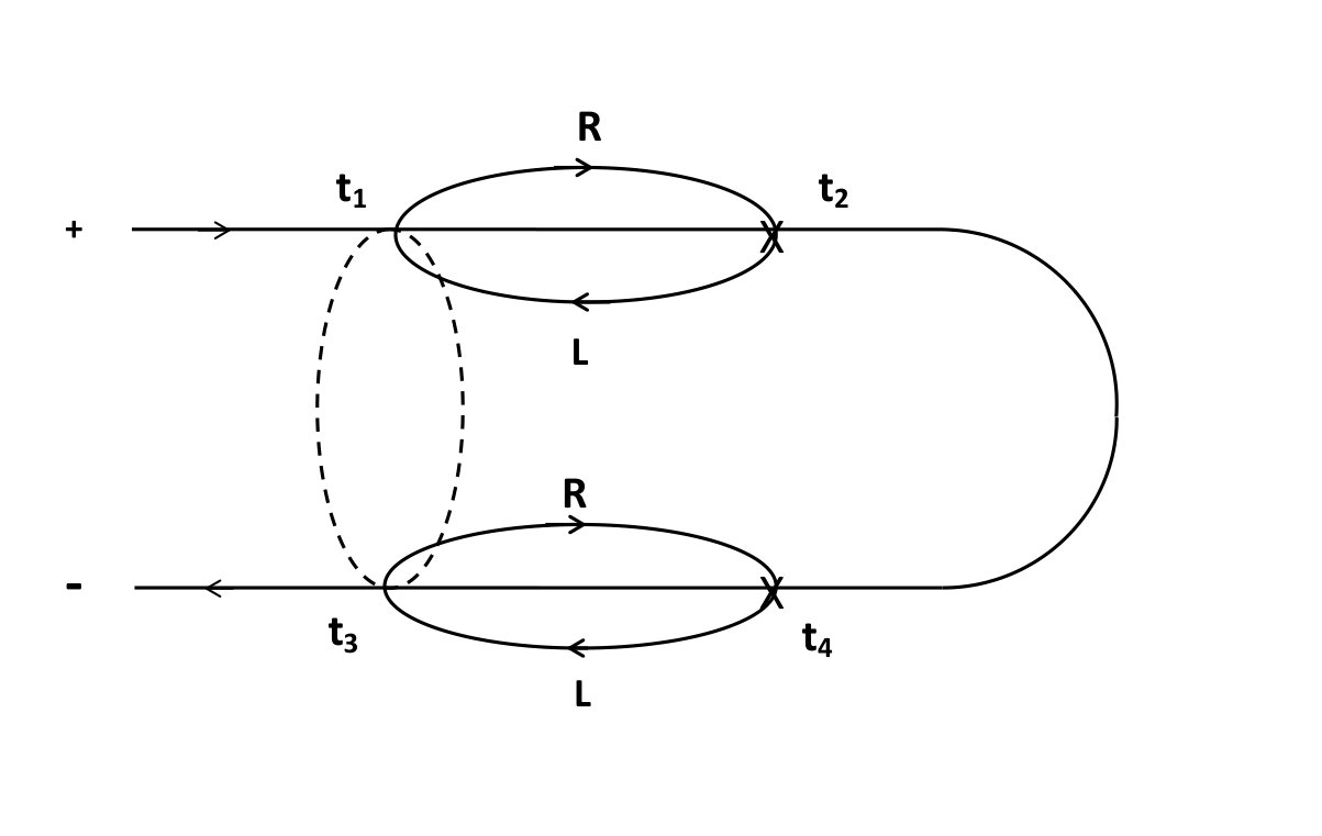 Figure 15
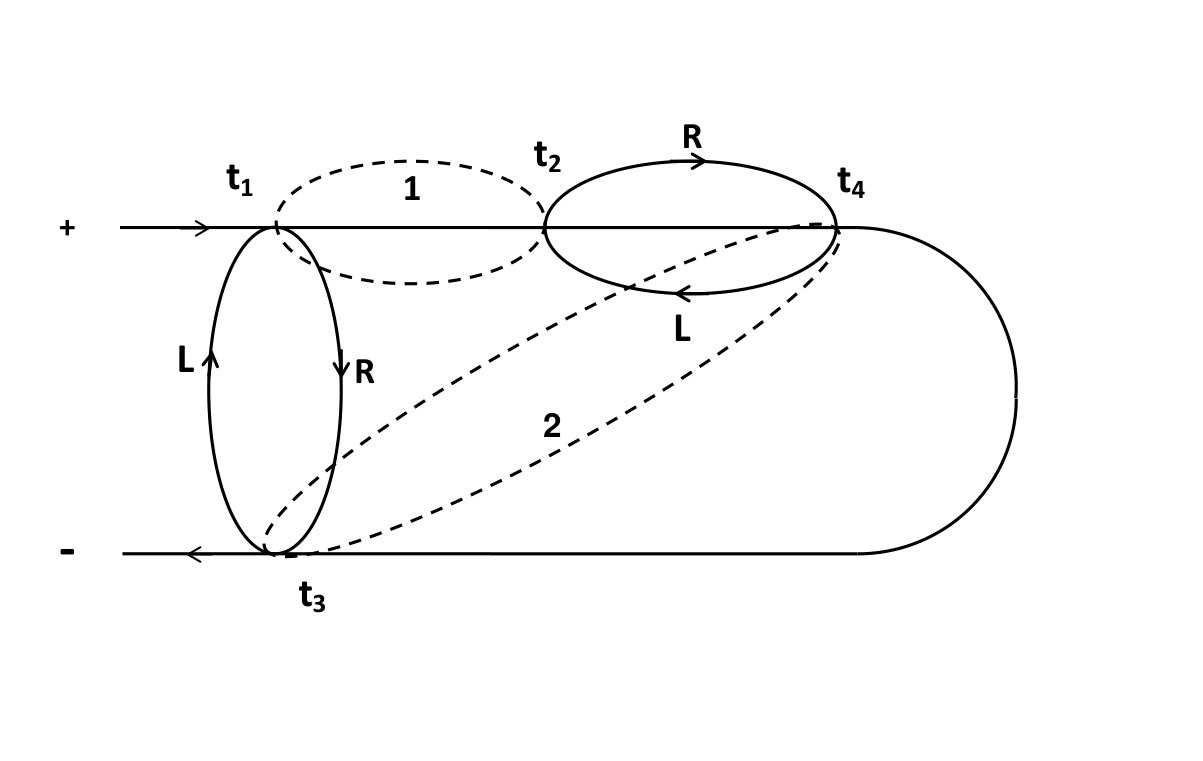 Figure 16
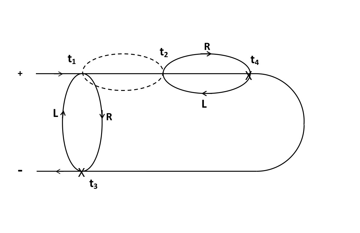 Figure 17
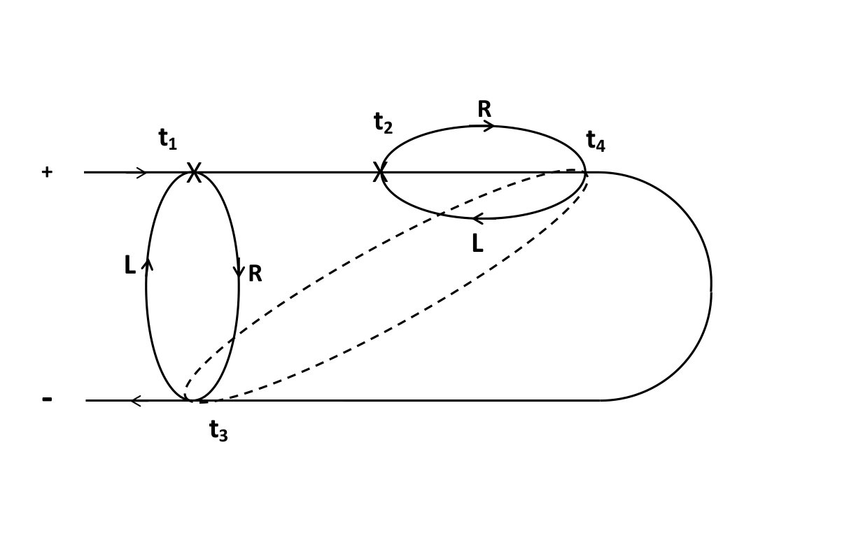 Figure 18
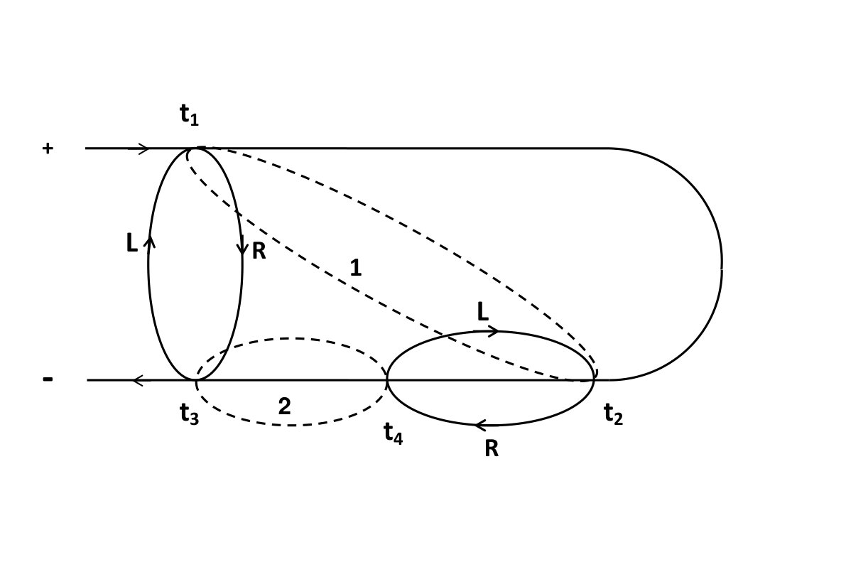 Figure 19
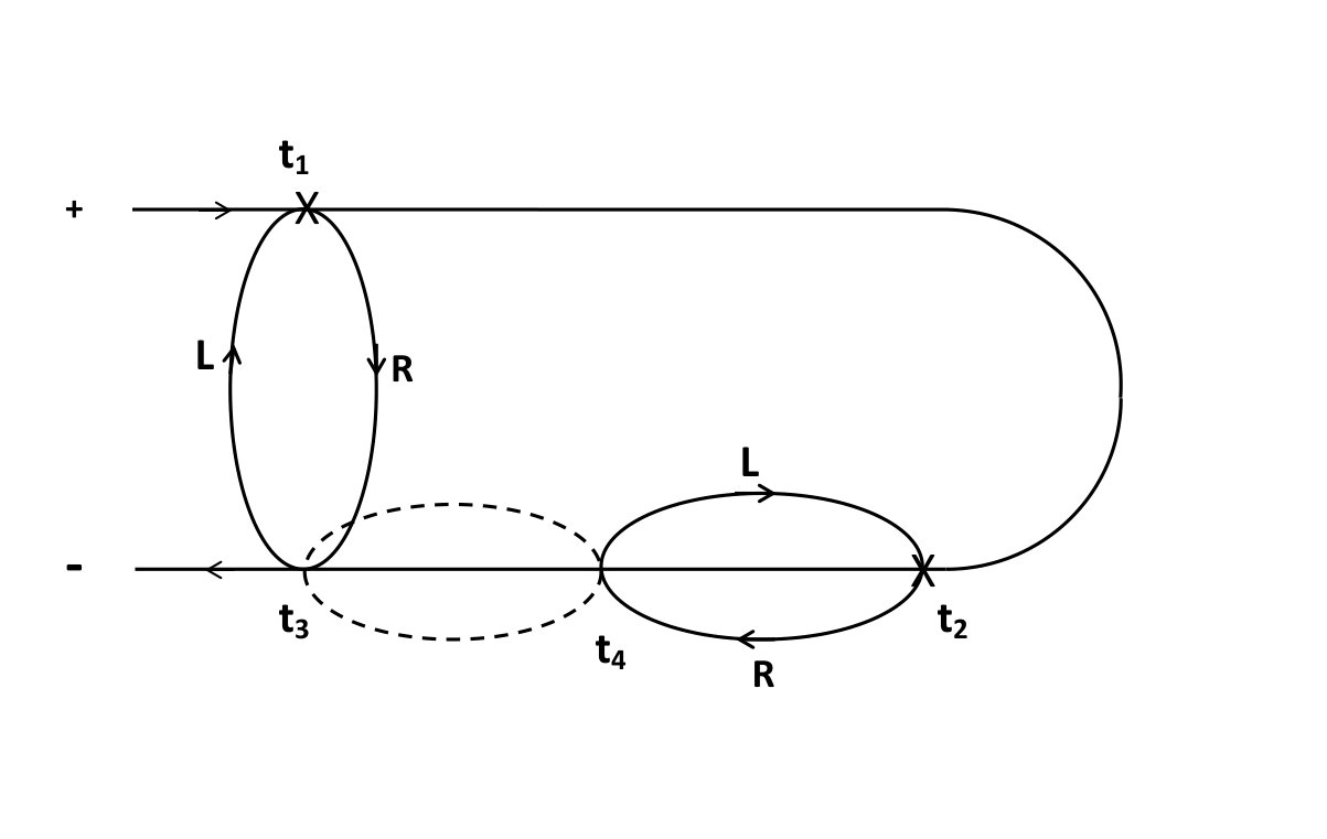 Figure 20
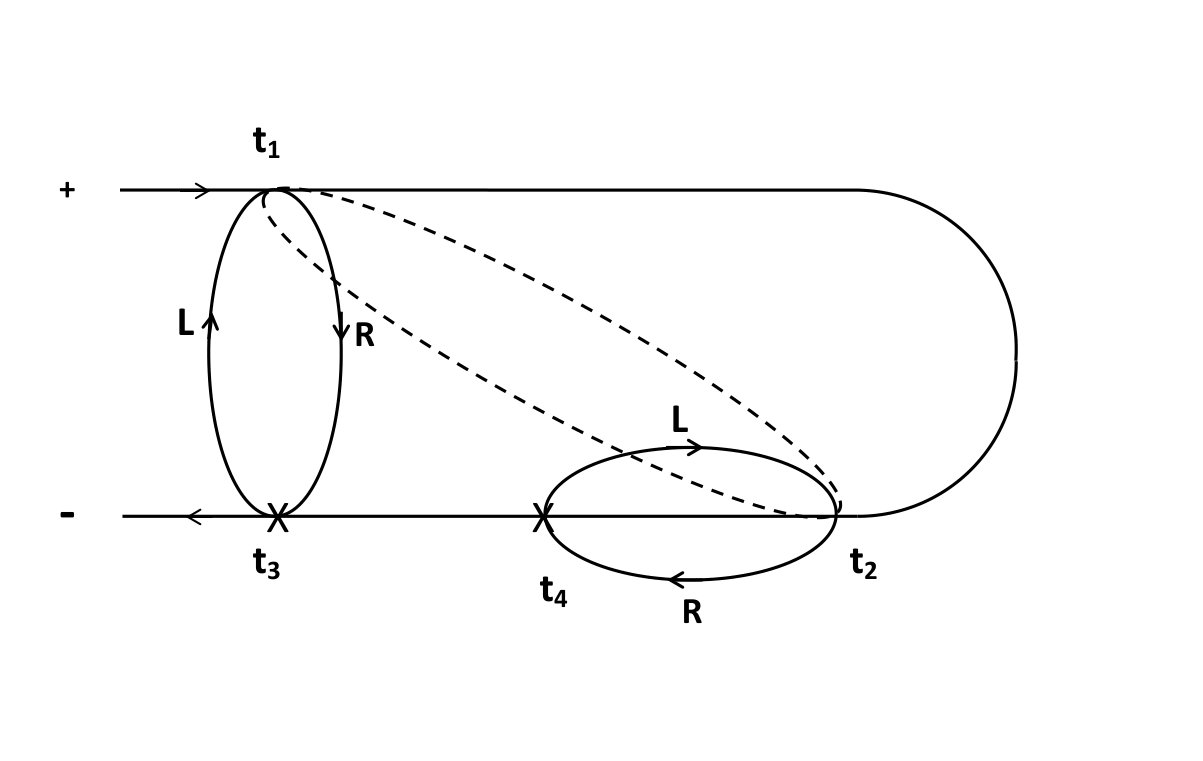 Figure 21
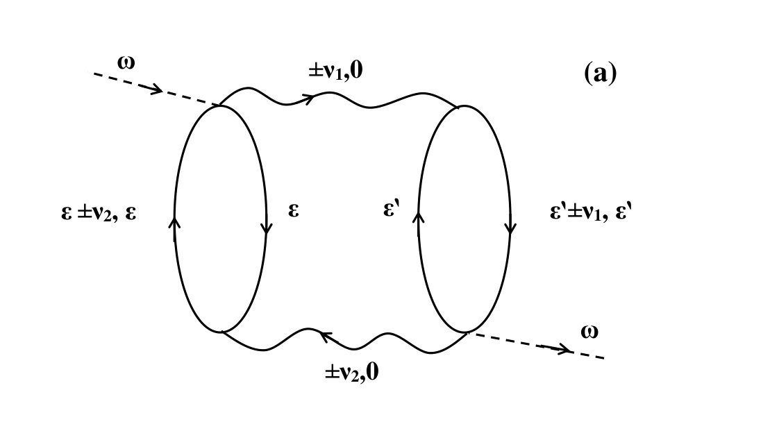 Figure 22
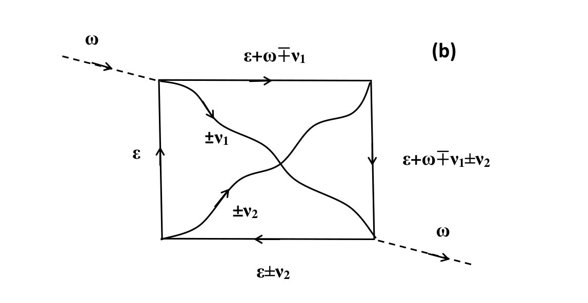 Figure 23
 Figure 24
| single spin + direct tunneling | Two spins | |||
|---|---|---|---|---|
| non-interacting | strongly interacting | non-interacting | strongly interacting (DQD) | |
| Linewidth | ||||
| DC current | ||||
| Resonance frequencies | ||||
| Fano factors F | & | |||
Peer Reviews
No public reviews on file for this paper yet. If you reviewed it on a platform where reviews are public (OpenReview, ICLR, NeurIPS, ICML), you can paste yours below so the community can read it here.
Videos
No videos yet. Explain this paper in a talk, walkthrough, or lecture? Add one.
Double Quantum Dot scenario for spin resonance in current noise
Baruch Horovitz and Anatoly Golub
Department of Physics, Ben Gurion University, Beer Sheva 84105 Israel
Abstract
We show that interference between parallel currents through two quantum dots, in presence of spin orbit interactions and strong on-site Coulomb repulsion, leads to resonances in current noise at the corresponding Larmor frequencies. An additional resonance at the difference of Larmor frequencies is present even without spin-orbit interaction. The resonance lines have strength comparable to the background shot noise and therefore can account for the numerous observations of spin resonance in STM noise with non-polarized leads. We solve also several other models that show similar resonances.
Coherent control and detection of a single spin are fundamental challenges in nanoscience and nanotechnology, aiming to determine electronic structures as well as provide qubits for quantum information processing koppens ; awschalom . Of particular interest are studies that combine the high energy resolution of electron spin resonance (ESR) with the high spacial resolution of scanning tunneling microscope (STM). These ESR-STM studies are of two types, either monitoring the current power spectrum in a DC bias manassen1 ; balatsky1 ; manassen2 , or monitoring the DC current when an additional AC voltage is tuned to resonance conditions mulleger ; baumann ; willke . In the latter case with a magnetic tip baumann ; willke the theory is well understood baumann ; shavit . In Ref. mulleger, the tip is apparently nonmagnetic, hence it should be interpreted as the inverse phenomenon to that of the first type.
We focus here on the ESR-STM phenomenon of the first type, i.e. a DC bias alone. The experimental technique is conceptually simple: an STM tip is placed above a localized spin center in presence of a DC magnetic field and the power spectrum, monitoring the current fluctuations, is measured; the data exhibits a sharp resonance at the expected Larmor frequency manassen1 ; balatsky1 ; manassen2 even at room temperature. This phenomena has been further confirmed by an associated ENDOR effect manassen3 . The understanding of this ESR-STM phenomenon presents a theoretical challenge even at present balatsky1 . It was proposed early on that a spin-orbit coupling is essential for converting the spin fluctuations to current noise, assuming also that the tip and substrate are spin polarized bulaevskii ; gurvitz ; martinek . However, the experimental data manassen1 ; balatsky1 ; manassen2 involves non-polarized tip and substrate. It was argued that an effective spin polarization is realized either as a fluctuation effect balatsky2 ; manassen2 or due to 1/f magnetic noise of the tunneling current manassen4 . The first theoretical model that conclusively showed an ESR-STM phenomena in this case, i.e. non-polarized electrodes in a DC setup, was a nanoscopic interferometer model caso ; golub . In this model the current has an additional channel of direct tunneling from the tip to the substrate in parallel to the current via the spin states. The interference between the two channels leads to an ESR resonance, however, the signal is rather weak. Furthermore this model ignores on-site Coulomb interactions, that are expected to be significant at a localized spin site.
In the present work we propose a new mechanism for the ESR-STM phenomenon, a mechanism that provides a strong signal, comparable to that of the background shot noise, and allows for a strong Coulomb interactions at the spin site. The model assumes the presence of an additional spin such that the current passes in parallel via two spins, i.e. a double quantum dot (DQD). The additional spin is unintentional in the ESR-STM experiments so far, yet its presence can be tested by monitoring our predictions. In particular, in addition to the expected resonance at additional resonances are present at and at ; are the g-factors of the two spins, respectively, is the Bohr magneton and is the DC magnetic field. We solve also the single spin model caso ; golub with strong on-site Coulomb repulsion, as well as the non-interacting two spin model. We find that the DQD model provides a strong signal to noise ratio and is most likely to account for the ESR-STM data. The properties of all the studied models are summarized in table I below.
We review first the previous model caso ; golub that involves interference between tunneling via the spin and direct tunneling, as illustrated in Fig. 1a. Consider (left, right) fermion leads (i.e. tip and substrate) with the Hamiltonian where denotes the spin and are continuum states; are the lead fermion operators whose dispersions include the voltage and are spin independent, justified by the small ratio of the Larmor frequency and a typical electron bandwidth. The spin site involves fermion operators and a Hamiltonian {\cal H}_{d}=\sum_{\sigma}(\epsilon_{0}+\mbox{\small\frac{1}{2}}\nu\sigma)d^{\dagger}_{\sigma}d_{\sigma} where is the (single) Larmor frequency with g-factor . The reservoirs are connected by a direct tunneling as well as by tunneling via the spin, the latter allows for an SU(2) spin-orbit rotation caso ; golub \hat{u}=\mbox{e}^{i\sigma_{z}\phi}\mbox{e}^{\mbox{\small\frac{1}{2}}i\sigma_{y}\theta} where are the Pauli matrices. The total Hamiltonian is with the tunneling term,
[TABLE]
where all operators are now spinors and is at the tunneling site. The current noise for this model has been solved exactly caso ; golub with results summarized in the first column of table I, yet it is instructive to derive the main results heuristically. The resonance linewidth is seen from a Golden rule , assuming now and the density of states per spin of both leads are taken equal, for simplicity. The resonance in the current correlation involves a closed loop with a given spin that passes at both spin levels, as illustrated in Fig. 1a. Hence one needs at least 6 tunneling events, 4 via the spin and 2 direct tunnelings, as well as two spin flips of probability \sin^{2}\mbox{\small\frac{1}{2}}\theta, hence an amplitude \sim t^{4}W^{2}\sin^{2}\mbox{\small\frac{1}{2}}\theta which multiplies a Lorenzian of width , hence the peak amplitude is \sim t^{4}W^{2}\sin^{2}\mbox{\small\frac{1}{2}}\theta/\Gamma\sim t^{2}W^{2}\sin^{2}\mbox{\small\frac{1}{2}}\theta. This derivation is valid if the spin levels are within the voltage window caso ; golub , i.e. |\epsilon_{0}|<\mbox{\small\frac{1}{2}}eV[1+O(T/eV)] at temperature . The direct current is also found by a Golden rule rate per spin times the final number of available states , i.e. . Assuming the background shot noise is , hence the Fano factor, i.e. the ratio of the resonance peak to that of the background, is F\approx\Gamma\sin^{2}\mbox{\small\frac{1}{2}}\theta/eV. For balatsky1 ; manassen2 MHz, eV this ratio is , too small to account for ESR-STM data. (If the Fano factor would be even smaller, ).
We consider next our new model, first its non-interacting variant. The model involves current transport via two spins, in parallel, i.e. the Hamiltonian is where are fermion spinor operators on the two spin sites,
[TABLE]
We assume that only the R electrode (probably the tip) has significant spin-orbit interaction. In fact this is equivalent to two SU(2) spin rotation matrices for tunneling from R to sites 1 and 2, respectively, i.e. . In general the wavefunctions of the two spins differ in their orbital part as well as in their locations, hence we expect . In the supplementary material SM we extend Bardeen’s formula to include spin-orbit coupling and estimate the spin-flip angle . We find that 0<|\tan\mbox{\small\frac{1}{2}}\theta|\lesssim 1, depending on the location of the spin site. Hence two spin locations can lead to fairly different . We then rotate so as to cancel in the term while for the term, resulting in Eq. (2).
The current fluctuations correspond now to Fig. 1b, i.e. a closed loop passing through both spins, at either level of each spin. A resonance appears then at the difference in energy levels, i.e. at \mbox{\small\frac{1}{2}}|\nu_{1}\pm\nu_{2}|; the sign is for trajectories through opposite (same) side levels. For a finite relative chemical potential there are more resonance lines at |\mbox{\small\frac{1}{2}}\nu_{1}\pm\mbox{\small\frac{1}{2}}\nu_{2}\pm\Delta|. The significant virtue of the process in Fig. 1b is that only 4 tunneling events are needed, hence a much stronger resonance. We present SM an exact solution of Eq. (LABEL:e02) with numerical plots of typical results. The solution can be expanded for weak tunneling, with results summarized in the 3rd column of table I. While the Fano factor is strong the model is inadequate since it neglects on-site Coulomb interactions, expected to be strong for the experimental realizations. Furthermore, the resonance frequencies depend on the unknown parameter. In fact, the addition of Coulomb interactions is essential for confining the dots as neutral so that the chemical potential becomes irrelevant.
We proceed now to solve both models Eqs. (I,LABEL:e02) when strong on-site Coulomb interactions are present, as indeed is the case in atoms and small molecules. Considering first Eq. (I), we add a term where . The effective Hamiltonian for large is well known from a Schrieffer-Wolff (SW) transformation hewson
[TABLE]
where is the spin operator, and an Aharonov-Bohm phase is introduced, useful in the following. may include potential scattering terms generated by the SW transformation. We note that is reduced by the strong Coulomb interaction, i.e. large and , an effect known as the Coulomb blockade. We keep in (12) only exchange terms that allow transport between the electrodes, other exchange terms that involve electrons only on one electrode are neglected since their contribution to transport would be of higher order. We perform SM a perturbation expansion to order using the Keldysh method. The result shows, surprisingly, that the resonance term precisely vanishes when . In ESR-STM experiments we expect since the nanometric dimensions of the setup allow only a negligible magnetic flux. To motivate this result, consider an interference along the loop and an additional trajectory of going around the loop in the opposite direction . When these trajectories are related by time reversal, the single spin in the loop then yields a relative minus sign, i.e. cancellation. More specifically, these two processes, when the localized spin is flipped up, sum up to
[TABLE]
where are Fermi functions and \mbox{Tr}[\sigma_{-}\hat{u}^{\dagger}]=-\mbox{Tr}[\sigma_{-}\hat{u}]=2\sin\mbox{\small\frac{1}{2}}\theta\mbox{e}^{i\phi}. Hence the interference cancels at . Energy conservation implies and integration on yields then an factor. Additional interference cycles that start at L involve are negligible for and . The result (13) is confirmed by detailed perturbation expansion SM , as summarized in the 2nd column of table I. Hence for the experimentally relevant case with this model may give a resonance only at orders higher than and therefore does not account for ESR-STM data. We note also that replacing in Eq. (13) yields a resonance at with amplitude \sim\mbox{Tr}[\sigma_{z}\hat{u}^{\dagger}]\mbox{e}^{-i\chi}+\mbox{Tr}[\sigma_{z}\hat{u}]\mbox{e}^{i\chi}=4\sin\chi\sin\phi\cos\mbox{\small\frac{1}{2}}\theta.
For completeness, we evaluate the resonance linewidth, relevant when . The simplest approach is a Golden rule for the decay of a spin up by passing an electron from L to R,
[TABLE]
Similarly for , so that , hence for the isotropic interaction in (12) the linewidth is . This result is confirmed by solving a Lindblad type equation SM for the spin dynamics; it is also consistent with the linewidth as derived by higher orders in Keldysh diagrams paaske , however, the framework of the Lindblad equation, being a proper 2nd order perturbation, is considerably more convenient. The Lindblad equation also shows a shift in the resonance frequency \delta\nu=-4\pi eVJWN^{2}(0)\sin\phi\cos\mbox{\small\frac{1}{2}}\theta\cos\chi, that may well be larger than the linewidth.
We proceed to our most interesting model, the DQD model with strong on-site Coulomb interactions. Proceeding with a SW type derivation SM we find that (LABEL:e02) is replaced by
[TABLE]
which is an obvious extension of the single spin case. This Hamiltonian neglects potential scattering terms that may generate terms beyond those that we study of order ; also here, for simplicity. Tunnelling between the two spin sites is neglected, leading to higher order terms for transport SM ; this tunneling yields also a direct exchange between the spins which shifts the Larmor frequencies, we neglect here this effect (e.g. if one spin is on the tip and the other on the surface this exchange is much weaker than either or ).
We note that the spin-orbit factor is essential for observing a resonance at a Larmor frequency. If then the tunneling elements conserve the total spin, while the terms in allow conservation of the z component of the total spin. Thus a closed loop of a lead electron returning to its original spin cannot flip a single spin, i.e. no resonance at either or . The loop can, however, flip both spins in opposite ways, hence a resonance at is possible even without spin-orbit effects. In fact, the same symmetry reasoning applies to all the models considered above. We further note that models with transport via a single spin, even if including spin orbit interaction, e.g. Eq. (15) with , do not show an ESR-STM phenomenon. This is seen by rotating so that is canceled and then total conservation rules out a spin-flip resonance. This conclusion holds for models with other types of isotropic exchange interactions manassen2 ; balatsky2 , interactions that commute with the total .
To appreciate the type of results, we consider the loops as in Eq. (13) which for a single spin flip involve on one spin while on the other, hence
[TABLE]
Hence we expect resonances of the form \sim J_{1}^{2}J_{2}^{2}\sin^{2}\mbox{\small\frac{1}{2}}\theta\delta(\omega-\nu_{i}), i=1,2. An additional resonance at appears when in Eq. (16), the matrix elements then lead to to 2\cos\mbox{\small\frac{1}{2}}\theta\mbox{e}^{i\phi}, hence a resonance \sim J_{1}^{2}J_{2}^{2}\cos^{2}\mbox{\small\frac{1}{2}}\theta\delta(\omega-|\nu_{1}-\nu_{2}|). One further resonance is possible at when in Eq. (16), i.e. no spin flips, leading to 4\cos\phi\cos\mbox{\small\frac{1}{2}}\theta, hence a resonance \sim J_{1}^{2}J_{2}^{2}\cos^{2}\phi\cos^{2}\mbox{\small\frac{1}{2}}\theta\delta(\omega). Finally, there is no resonance at since .
We proceed now to our diagrammatic expansion. First, consider skeleton diagrams, i.e. without Keldysh indices, that show readily which type of diagrams to 4th order can produce a resonance. Fig. 2a shows a typical diagram that has a resonance, i.e. frequency conservation at each vertex yields readily function resonances at and [math]. In contrast, Fig. 2b shows that all spin frequencies merely shift an electron energy which is being integrated. Hence a weak dependence, i.e. a non-resonant effect. [We note that similar skeleton diagrams can be constructed also for our single dot model Eq. (12), one spin line is eliminated while its vertices remain as the direct tunneling term.]
We present a detailed Keldysh diagrammatic expansion SM . The results are consistent with the reasoning above and are summarized in the 4th column of table I. We also solve SM a Lindblad equation for this case to identify the various linewidths of the various resonances , leading to
[TABLE]
This result is similar to that of the single spin case obtained from Eq. (14), except that each spin is affected also by the longitudinal relaxation of the other spin; furthermore, the resonance includes a non-secular term SM .
The DC current is given in table I, as expected it is , so that the background shot noise is . The resonance signal at maximum is obtained from the discussion following Eq. (16) and is confirmed by the diagrammatic expansion SM , with the replacement . The ratio of this peak value and that of the background is given for in the table while for the other resonances it is ,
[TABLE]
We note that the resonance at is strongest without spin-orbit coupling, i.e. , with a relatively narrow linewidth.
We consider next the relevance of our results to the experimental situation manassen1 ; balatsky1 ; manassen2 . First, we note that the data shows a sharp resonance even at room temperature. This is fully consistent with our results since the linewidth is dominated by the voltage with . Second, we note that the linewidth of 25MHz at nA manassen3 implies that the DC current via the spins (table I) is nA, much smaller than the total current. We expect then that most of the current tunnels directly between the tip and substrate, indeed a dominant tunneling as it is not Coulomb blockaded. We expect that this current is incoherent with those via the spins, otherwise it would lead to a large shift in the resonance frequency (see paragraph below Eq. (14)). Finally, the ratio of peak noise power to that of the shot noise has been estimated manassen2 as , however, since the power spectrum is measured via modulation of the magnetic field its absolute value has not been so far directly measured.
These experiments manassen1 ; balatsky1 ; manassen2 aim to probe a known spin site on a surface. We propose that a second spin is present, allowing for the observed strong signal. The most likely location for the second spin is on the STM tip which is usually made of a heavy metal with significant spin-orbit coupling. Indeed, the presence of dangling bond surface states in various tip materials is known chen , such states are candidates for spin sites. By extending the measured frequency range, we predict the observation of a second Larmor frequency as well as a signal at a lower frequency . The latter in fact may well be stronger than those at either or if the spin-orbit effect is weak, i.e. small . We note that preliminary data shows a strong signal at low frequency for either defects on a SiC surface or for Tempo molecules on Au substrate manassen4 .
We note finally that the second type of ESR-STM, i.e. enhanced DC current at resonance with an applied AC voltage baumann ; willke involves a magnetized Fe atom on the tip. While this is superficially similar to our 2-spin scenario, it is a fundamentally different mechanism, being based on a permanently strong magnetic atom. In our scenario both spin sites exhibit spin fluctuations, in fact even the average spin of each site is extremely weak SM ; yet, data on noise in the spin current might show similarities.
In conclusion we have solved a number of models showing an ESR-STM phenomenon, concluding that the model of two spins with strong on-site Coulomb interactions is the most likely to account for the data. Observation of our prediction for additional magnetic field dependent frequencies in the power spectrum would be the clearest support for our mechanism.
Acknowledgements.
We thank Y. Manassen for illuminating discussions on his data and the experimental setup. We also thank C. P. Moca, G. Zaránd and Y. Meir for stimulating discussions. BH also gratefully acknowledges funding by the German DFG through the DIP programme [FO703/2-1].
I Spin orbit matrix
In this section we first extend Bardeen’s formula bardeen for tunneling to include spin-orbit and then we use this formula to estimate the parameters of the spin rotation matrix . In particular we consider tunneling from the STM tip to a spin site and show the dependence of the SU(2) matrix on the position of the spin site.
The extension of Bardeen’s formula to include spin-orbit caso is derived here in more detail. Consider a curved surface , labeled here as a coordinate , that separates Hamiltonians with potentials for the left and right terminals of the tunneling, respectively, e.g. is the tip and is a spin site,
[TABLE]
where is the spin-orbit coupling, is the local electric field and is the spin operator, e.g. Pauli matrices for spin .
Consider spinor wavefunctions which solve with degenerate eigenvalue , describing elastic tunneling. The separating surface is chosen such that are localized on the sides, respectively, i.e. decay exponentially into the opposite sides and their overlap is small. Perturbation theory for weak tunneling considers the eigenstate of the full Hamiltonian in the form with a shifted eigenvalue , hence
[TABLE]
where we neglect terms with two decaying eigenfunctions as well as a product with an overlap term which is of higher order. Defining the tunneling elements as , then as shown below and the equation above determines and .
We proceed to evaluate . Taking the Hermitian conjugate of we can rewrite, avoiding here partial integration,
[TABLE]
Using for and (static fields),
[TABLE]
The first term gives Bardeen’s formula
[TABLE]
The spin-orbit term reduces also to a surface term
[TABLE]
To obtain the tunneling we need repeat the previous calculation with and integrating on . Hence with
[TABLE]
since the normal to the surface is now in the opposite direction . The spin-orbit term is
[TABLE]
Hence .
We next estimate the spin rotation angle as defined by \hat{u}=\mbox{e}^{i\sigma_{z}\phi}\mbox{e}^{\mbox{\small\frac{1}{2}}i\sigma_{y}\theta}. We note first that the tip wave function is localized at the tip apex, hence the surface varies on an atomic scale chen so as to minimize the overlap between the states ; the surface can be taken as a semi-circle around the tip apex chen . Furthermore, The surface integrals for both are dominated by a point where the overlap of the localized wavefunctions is maximized. This point is the closest one to the position of the spin site. Hence
[TABLE]
where is a unit vector perpendicular to the surface at and is a combined decay length of the localized states, an atomic scale.
A further input are the equipotential lines in an STM set up devel . The STM tip consists of an atomically sharp apex that is supported by a tip body of a much larger scale, i.e. 20-100nm. The equipotential lines have therefore a sharp component as well as a smooth one on the larger scale. Therefore has a component in the direction, perpendicular to the substrate, while , chosen to be in an plane, has an angle relative to the axis, pointing towards the spin site. This estimate yields
[TABLE]
Finally, we need to estimate the spin-orbit coupling . We consider Tungsten (W) as a representative material for an STM tip. Data shikin on clean W(110) and on one monolayer H on W(110) show a spin-orbit splitting of eV at wavevector . Further data rotenberg on W(110) shows a spin-orbit splitting of eV, increasing to eV with 0.5 monolayers of Li, reflecting an enhancement of the W spin-orbit by the electric field induced by the Li coverage rotenberg . We infer that eVcm, a value that is likely to be enhanced by the strong electric field in an STM setup. Taking 1nm we obtain with the latter that \tan\mbox{\small\frac{1}{2}}\theta\approx 3\sin\beta. Hence the spin flip angle, as well as the matrix have a strong dependence on the location of the spin. In the case of two spin sites, their different locations would lead to different matrices . If the spin sites correspond to different types of atoms or molecules, then the different decay length would also cause a difference between their matrices .
II Current noise – noninteracting case
We study here the 2-spin system as given in Eq. (2) of the main text. We use the rotated Keldysh basis kamenev so that the action of the right (R) and left (L) leads is
[TABLE]
where the Greens functions (GF) involve the retarded , advanced and Keldysh components , in units of the right or left density of states (assumed equal for simplicity), are
[TABLE]
where corresponds to , respectively. [We note, however, that care is needed if the combination appears, e.g. ].
The tunneling part of the action includes a quantum source that couples to the current operator and to a Pauli matrix in the rotated Keldysh basis
[TABLE]
The source represents the quantum source kamenev field which is set to zero after variations that define either the current or the noise power. (The source here couples symmetrically to the left and right lead currents, hence a factor is inserted in the following for each current).
The electron operators of the leads can be integrated out, leading to an effective action in terms of dot electrons, represented as a spinor ,
[TABLE]
where correspond to respectively. Each Keldysh element of the self energy is a matrix in the spin site index, resulting in
[TABLE]
Here ; and j=1(2) correspond to L(R) lead. Note that is a matrix in Keldysh space and is obtained by products of matrices and the GF of the leads, Eq. (II). We assume here and for simplicity, and define as well as .
Taking variation with respect to the quantum source we find the transport current I and the noise power spectrum ,
[TABLE]
In these formulae integration over each time variable is implied except of and . From equations (32, 35) the inverse retarded Green function is identified as a matrix or explicitly
[TABLE]
The Keldysh components of the GF are identified by taking the inverse of (32) at , which implies that are inverses of , respectively, while
[TABLE]
The first variation of the self energy M takes the form
[TABLE]
By taking the trace in Eq.(36) over Keldysh space we obtain the current
[TABLE]
The part of noise power incudes second variation of self energy
[TABLE]
The trace of in Keldysh space may be written, with a shorthand notation , as . Using explicit expression for Keldysh components of M we calculate :
[TABLE]
Our main interest is the experimental situation with large voltages , then does not depend on frequency.
We consider next the noise using (38). With a shorthand notation the trace becomes
[TABLE]
Decomposing we define terms with the same type of two GFs (advanced or retarded) as , terms that include two Keldysh GFs and also terms which have one advanced and one retarded dot GF as , while the remaining terms stand for . Thus we obtain
[TABLE]
where .
For large voltage we can simplify expressions for current and . To do this we notice that in the limit and
[TABLE]
Note that becomes constant so that . We also find
[TABLE]
We note that in the absence of spin orbit scattering () the matrix and noise is just the independent , i.e. no resonance as expected.
We wrote a Mathematica program for evaluating the Fano factor
[TABLE]
First we show in Fig. 1 the saturation of the Fano factor at small occuring at for both high energy resonances and the low energy resonance at . Fig. 2 shows the resonance splitting due to , Fig. 3 shows the splitting due to while Fig. 4 shows splittings due to both effects, using a smaller where the high frequency resonances are weaker.
Finally, we consider the limiting case of small . Since the dominant term is the second one in Eq. (63) for , i.e.
[TABLE]
In this limit we consider only diagonal terms of in Eq. (39) (in the diagonal terms is kept infinitesimal), hence
[TABLE]
Using these GFs and taking the trace in Eqs.(67, 68) we obtain and .
The trace has a form:
[TABLE]
with all first GFs depend on and second ones depend on . Hence
[TABLE]
Performing the integration with we finally obtain
[TABLE]
We note that the linewidth defines the width of the GFs in Eq. (LABEL:Gmin). Since the power spectrum is a convolution of two such Lorenzians its linewidth is , i.e. Eq. (74) involves at each resonance
[TABLE]
In table I of the main text the of this section is replaced by \mbox{\small\frac{1}{2}}\Gamma to agree with the definitions of the other cases.
The power spectrum at resonance is then (apart of the dependent factors) so that the Fano factor, i.e. dividing by , has , as summarized in the 3rd column of table I in the main text.
III Schrieffer-Wolff transformation – double QD
We derive the Schrieffer-Wolff transformation (SW) by Hewson’s method hewson of performing a perturbation expansion directly on the Hamiltonian. We also assume that double occupancy of the dots is forbidden (infinite ) while the ionization potentials are finite and large. Transport is then allowed by first ionization and then recharging from the leads (co-tunneling). This simplifies the algebra, while capturing the essential form of the transformed Hamiltonian.
The 2-dot problem with 2 leads , including spin-orbit represented by an SU(2) matrix is given by the Hamiltonian, with operators as spinors,
[TABLE]
In the limit consider the subspace , (2-spinor), (2 spinor), (4 spinor). The Hamiltonian has the form
[TABLE]
The 1st line of (LABEL:e16) yields in terms of the other states,
[TABLE]
Substituting in the 2nd line yields
[TABLE]
The terms are of order and could be neglected in leading order in , yet it is of some interest to keep the term as it describes induced tunneling between the spins
[TABLE]
The 3rd line with solution (91) for is
[TABLE]
Now ignore the term and keep representing ,
[TABLE]
Finally can be written in terms of using their leading terms and then the 4th line of (LABEL:e16) can be written in terms of to identify the effective Hamiltonian,
[TABLE]
The terms yield a product of and 4 fermion operators with a coefficient which is smaller than even the 2nd order of the other terms, hence is neglected. If , a c-number tunneling term in the original Hamiltonian with , then it yields and similar terms with . To 4th order it is much smaller than the terms that we keep (), while to 2nd order it does not give a resonance.
We note that when all are finite and large, a process of tunneling from e.g. the first neutral dot to the second one yields a term with . This yields higher order corrections to the transport, however it may affect the eigenfrequencies of the 2-dot system. We assume here that this effect is negligible; in particular in the scenario that one spin is on the tip and the other on the surface we have , hence , being the exchange terms responsible for the resonances (see (98) below).
To identify the result in terms of spin operators we note an identity for spinors on either lead and spinors on either dot with spin operators {\bf S}_{i}=\mbox{\small\frac{1}{2}}d_{i}^{\dagger}{\bm{\sigma}}d_{i} defined on singly occupied dots,
[TABLE]
which can be shown by using rotated fermions, e.g. , also are either or . Using then and assuming we obtain
[TABLE]
We note that multiply in the subspace, hence these are constant terms and do not participate in the excitation spectrum (98).
It is important to note that without the spin-orbit effect, i.e. if , then the total z component spin is conserved. This is seen by the scalar product that for any spin flip of the dot involves an opposite spin flip of the tunneling electrons. In fact, the original form (III) commutes with , i.e. independent of the Scrieffer-Wolff procedure.
The conservation of implies no resonance at or in the noise spectrum since a resonance with a single spin flip implies that is not conserved. Hence a spin-orbit term is essential for the observation of these resonances. Two opposite spin flips are allowed, i.e. the resonance at can be seen even without spin-orbit.
IV Current Noise via Keldysh – double QD
IV.1 Tools
Assume so that current flows to the right, i.e. electrons flow to the left and . With the choice , the current operator is obtained by
[TABLE]
Since spin operators do not satisfy Wick’s theorem it is convenient to represent them by Abrikosov pseudofermions abrikosov ; moca for spin site and spin component ,
[TABLE]
where are the Pauli matrices. To the 4th order that we need one can in fact use spin propagators, since all diagrams involve pseudofermion closed loops (e.g. Fig. 7), yet we present the calculation with pseudofermions, anticipating higher order extensions in the future. The operators are replaced on the Keldysh contour (e.g. Fig. 7) by Grasmann variables where , while . For evaluating the leading order in the noise we keep only the transfer terms with spin,
[TABLE]
where are the Larmor frequencies and in the interaction term are at , i.e. . Eventually to enforce single occupancy of each of the psudofermions. Note that are spin independent. The current is
[TABLE]
The Green’s functions on the Keldysh contour is given by kamenev
[TABLE]
where, defining ,
[TABLE]
Similarly, for the pseudofermions,
[TABLE]
where in each term only the leading order in is kept. We expect that eventually the kept terms will cancel with the normalization .
IV.2 Diagram Rules
Vertices: each vertex carries a factor of either or ; The sign is for the current source of and for and is the same on both contours (to generate the quantum part), is for interaction vertex on the contour and on the contour (recall ).
The n-th order has n+2 vertices, two of which correspond to current terms (sources) with external variables, while n vertices have internal that are integrated upon. The first external time is on the contour and the second is on the contour; this generates . [This is sometimes moca denoted as ; the symmetrized form is obtained, after Fourier, by ]. Since the interactions and current terms have the same form one can choose in each diagram various combinations for the external vertices. Hence it is more compact to define diagrams in real time and later identify the various options for the external frequency.
Lines: Greens’ functions are full (dashed) lines for a () product, with the direction chosen kamenev to be in the direction from to ( to ), the Greens’ function argument is . The direction is conserved across each vertex (particle conservation). Each vertex connects to 4 lines – 2 outgoing full and dashed, 2 incoming full and dashed. There are 4 types of Greens’ functions:
A line connecting vertices within the contour is ().
A line connecting vertices within the contour is ().
A line connecting to contours, i.e. goes down, is ().
A line connecting to contours, i.e. goes up, is ().
A closed fermion or pseudofermion loop has an additional sign (one in the loop needs to be reordered).
Finally, to generate a single factor (projection on a singly occupied pseudofermion space) need one, and only one, of 3 factors: a single , a single with or a single with . (Note that in can be neglected since to close a loop an must be present). Hence the pseudofermion lines must be time ordered along the Keldysh contour.
IV.3 Traces
Consider here traces needed in the following for the quantity (which implicitly depends on ),
[TABLE]
The traces involve the electron spin operators while are matrices for the psudospin operators. Using the definition \hat{u}=\mbox{e}^{i\sigma_{z}\phi}\mbox{e}^{\mbox{\small\frac{1}{2}}i\sigma_{y}\theta} we obtain
[TABLE]
Define next where indices are summed as indicated on the right,
[TABLE]
Collecting all terms, i.e. summation on yields
[TABLE]
IV.4 Order n=0
To order the current operators we choose the first on contour at , the second on contour at , see Fig. 7. The signs involve on the and for the vertices. Hence the noise is (the numbers on top of each field are paired to show contractions, terms with and with to be added below))
[TABLE]
since are diagonal and spin independent, while are diagonal and spin dependent. Using Pauli matrix identities
[TABLE]
Therefore
[TABLE]
where . The voltage is assumed large so that and the integration range for which gives , where is the density of states (per spin) in the leads. The term with has is much smaller by order and is neglected. Finally, dividing by the normalization and then adding the term with we obtain
[TABLE]
Note that the DC current is
[TABLE]
IV.5 Order n=2
We look for interference between two spin, the lowest order is , i.e. 4 vertices with at least one on each contour. We keep only diagrams that have separate electron loops, other types do not lead to resonances (see Fig. 2b in the main text), thus the diagrams in Fig. 8 are neglected.
Consider first the diagram of Fig. 9; overall sign is from currents and from interactions,
[TABLE]
Here belong to spin 1 while belong to spin 2.
[TABLE]
Consider with external so give 3 independent functions with where , hence
[TABLE]
The product of the principal parts is weakly dependent, the imaginary part cancels with the term (see below), hence its real part is
[TABLE]
Integrating the four electron energies for
[TABLE]
where is evaluated above in Eq. LABEL:e209. As argued for Fig. 2a of the main text, this diagram indeed shows resonances.
Next is with external currents in , give 3 independent functions with . This is very similar to ,
[TABLE]
The product of the principal parts is weakly dependent, the imaginary part cancels with the term (see below), hence its real part is
[TABLE]
The divergence due to is studied in the summary below. Other options for external currents are included in the 2 cases above by smoothly interchanging the two bubbles, which is included in the time integrations.
Consider next where spins . The interchange implies that the spin-orbit matrix is now in vertices with (instead of at with ), hence the traces become . Also now belong to spin 2 while belong to spin 1. To revert to the previous notation relabel , hence need and as well as . This yields the same spin indices as in Eq. (LABEL:e55) with and the traces replaced by . Note which happens to be real (subsection C), therefore . Now change in the last form in Eq. LABEL:e54 and so that all functions regain the form as in LABEL:e54 and
[TABLE]
Furthemore, is defined as an ingoing frequency on the upper times , with the change of time variables it needs , hence for both we have . Interchanging the integration variables , and noting that is invariant under this, shows that ,
Consider now the crossed diagram Fig. 10,
[TABLE]
Interchanging and noting as all traces are real (subsection C) the coefficient is the same as above. Consider with external so give 3 independent functions,
[TABLE]
Consider with external so give 3 independent functions,
[TABLE]
Next is with external so give 3 independent functions,
[TABLE]
Finally with external so give 3 independent functions,
[TABLE]
Interchanging 1,2 is not needed since it is equivalent to shifting the two electron bubbles and reversing their positions which is included in the time integration.
Consider in Fig. 11, sign assumes that external currents are at () and at ()
[TABLE]
Defining ,
[TABLE]
Consider with yielding 3 independent functions with , hence
[TABLE]
Consider next with yielding 3 independent functions with (note opposite sign as current has now ), hence
[TABLE]
Consider next with yielding 3 independent functions with , hence
[TABLE]
Consider next with yielding 3 independent functions , hence
[TABLE]
Add 2 terms
[TABLE]
All terms with a single fermi function can be integrated on either or leading to which cancel, hence ignoring these terms
[TABLE]
The next 2 terms add up to
[TABLE]
Again, all terms with a single fermi function can be integrated on either or leading to which cancel, hence ignoring these terms
[TABLE]
The same separation can be done on the variables, ignoring terms that eventually cancel in the integrations ( terms)
[TABLE]
The integration has and similarly for the integration. These terms are negligible for .
Finally for , in each fermion bubble one can change independently (without changing spin label), which changes the sign of and/or in the result (LABEL:e77). All these 3 versions are negligible in the same way.
Consider now , Fig. 12, sign assumes that external currents are at ,
[TABLE]
Multiply first the two and then Fourier,
[TABLE]
For need yielding 3 independent functions with
[TABLE]
The 1st P.P. vanishes since by integrating either or . The 2nd P.P. is then an imaginary term that cancels (see below), so remains the product of functions
[TABLE]
which is divergent when .
For need yielding 3 independent functions with , hence
[TABLE]
The 1st P.P. vanishes as in (LABEL:e80), while the 2nd P.P. is then an imaginary term that cancels (see below), so remains the product of functions
[TABLE]
For need , it has a relative to since current couples to . It yields 3 independent functions with
[TABLE]
The 1st P.P. vanishes as in (LABEL:e80), while the 2nd P.P. is then an imaginary term that cancels (see below), so remains the product of functions
[TABLE]
Both have resonance , however for they cancels.
We note that in the ordered fermion bubble is identical to the result above except for , and a sign change in that have a current vertex on this bubble. Hence for large this yields a factor 2 in while both cancel. Before considering spin exchange , we study Fig. 13.
The sign for assumes external currents at .
[TABLE]
For need , it yields 3 independent functions with , hence
[TABLE]
The 1st P.P. vanishes as in (LABEL:e80), while the 2nd P.P. is then an imaginary term that cancels (see below), so remains the product of functions
[TABLE]
This has a divergent .
For need , it yields 3 independent functions with , hence
[TABLE]
The 1st P.P. vanishes as in (LABEL:e80), while the 2nd P.P. is then an imaginary term that cancels (see below), so remains the product of functions.
For need , with a relative to , it yields 3 independent functions with , hence
[TABLE]
The 1st P.P. vanishes as in (LABEL:e80), while the 2nd P.P. is then an imaginary term that cancels (see below), so remains the product of functions. Both have resonance , however for they cancel. As for diagram 7, in the ordered fermion bubble is identical to the result above except for and a sign change in , hence a factor 2 for while both cancel.
Consider next where spins . Exactly as for below Eq. (LABEL:e62), the interchange implies that the spin-orbit matrix is now in vertices with (instead of at with ), hence the traces become . Also now belong to spin 2 while belong to spin 1. To revert to the previous notation relabel , hence need and as well as . This yields the same spin indices as in Eq. (LABEL:e78) with and the traces replaced by . Note which happens to be real (subsection C), therefore .
Consider from (LABEL:e80) with ,
[TABLE]
From (LABEL:e88) , which is just relabeling indices of the same spin, hence summation on spin indices allows keeping only the real parts. Similarly and . This is not essential since anyway would cancel.
Finally from (LABEL:e87) with ,
[TABLE]
so that , similarly and , allowing to keep only real parts.
**Aharonov-Bohm phase
**
We comment now on the modification due to adding a Aharonov-Bohm phase in the Hamiltonian, i.e. . Note first that for Eqs. (LABEL:e57,LABEL:e61) terms with a single P.P. involve that has a real part which does not cancel with ; yet, this term is and a similar term without , these are weakly dependent, i.e. they are not a resonance, and are neglected. Same with the P.P. for , Eqs. (LABEL:e80,LABEL:e82,147) and , Eqs. (LABEL:e87,LABEL:e89,LABEL:e90). Therefore, the noise terms and are multiplied by , while all terms of are not changed. All terms acquire while for their exchange the phase cancels, hence S_{7a}\rightarrow\mbox{\small\frac{1}{2}}S_{7a}(\mbox{e}^{-2i\chi}+1); together with the h.c. term we have a factor \mbox{\small\frac{1}{2}}(\cos 2\chi+1). acquire a factor \mbox{\small\frac{1}{2}}(\mbox{e}^{-2i\chi}-1), but anyway these two cancel , same with and the primed quantities.
IV.6 Summary – two QD
Consider first the divergent terms, in exchange integration variables since is symmetric in these.
[TABLE]
where in the factor is neglected for and large. In the generic case the factor implies . The divergence cancels exactly (!) (even for ), again using in .
We proceed finally to our main result with the resonance terms in which before normalization are
[TABLE]
Recall \lambda_{i}=\lambda_{0}+\mbox{\small\frac{1}{2}}\gamma_{i}\nu_{1}\,(i=1,2),\,\lambda_{i}=\lambda_{0}+\mbox{\small\frac{1}{2}}\gamma_{i}\nu_{2}\,(i=3,4). Using the result for Eq. LABEL:e209 and summing on (each line indicates near its end the values of ), we have before normalization,
[TABLE]
It is remarkable that the terms vanish, i.e. no resonance at . Finally, normalize by (\mbox{e}^{-\mbox{\small\frac{1}{2}}\beta\nu_{1}}+\mbox{e}^{\mbox{\small\frac{1}{2}}\beta\nu_{1}})(\mbox{e}^{-\mbox{\small\frac{1}{2}}\beta\nu_{2}}+\mbox{e}^{\mbox{\small\frac{1}{2}}\beta\nu_{2}}) to obtain
[TABLE]
V Current Noise via Keldysh – single QD
V.1 Tools
Consider noise for the J-W model, i.e. the effective action and current are
[TABLE]
represents an Aharonov-Bohm phase.
The diagram rules are similar to those of the double QD case except for a new type of vertex, denoted as X in the figures, where an L electron is directly transferred to an R electron, or vice versa, with strength .
We evaluate now a few traces, needed in the following:
[TABLE]
Define , note that all Tr are imaginary,
[TABLE]
V.2 n=0
From Fig. 14, for large and using ,
[TABLE]
adding the J term from Eq. (117). The DC current is
[TABLE]
V.3 Order n=2
From Fig. 15, left side,
[TABLE]
This is identical to in (LABEL:e54) except traces that are replaced by and that is missing. The latter is achieved by in the results. Hence from (LABEL:e57)
[TABLE]
From (LABEL:e61) with
[TABLE]
Consider next Fig. 15, right side,
[TABLE]
By it is seen from (LABEL:e104) that , noting that is invariant under . Furthermore, is defined as incoming on the upper times , hence the change in time variables needs, for both that . Hence the terms in (LABEL:e105), (LABEL:e106) involve while the P.P. terms involve . The latter are actually neglected since e.g. , i.e. these are not resonance terms (yet this term is asymmetric around a resonance, so might be of some interest).
Consider next Fig. 16, which is independent.
[TABLE]
Comparing with (LABEL:e64) shows that it needs to obtain . Hence from Eqs. (LABEL:e65-LABEL:e68)
[TABLE]
Consider next Fig. 17.
[TABLE]
This equals if and . Hence , Eq. (LABEL:e77), with an overall factor , shows then that is negligible for . Fig. 17 with in either bubble involves either or , yet summation on the 4 options of external sources leads to cancellation of either term, as in (LABEL:e77).
Consider now Fig. 18, sign assumes that external currents are at ,
[TABLE]
This equals in (LABEL:e78) if and ( since here ). Hence from Eqs. (LABEL:e80, LABEL:e82, 147), where the 1st P.P. vanishes and the dominant term at is
[TABLE]
where the additional terms in arise from the in the ordered fermion bubble as obtained from the result above except for ; however one trace involves (leading to ), but also a sign change for a current vertex for (leading to ). The terms with or are neglected, being much weaker than resonance. Note that for the sum .
Consider next Fig. 18 right side,
[TABLE]
This is obtained from (LABEL:e78) by and then replacing , and . Hence from from Eqs. (LABEL:e80, LABEL:e82, 147), where the 1st P.P. vanishes and the dominant term at is
[TABLE]
where the additional terms in arise from the in the ordered fermion bubble as obtained from the result above except for ; however one trace involves (leading to ), but also a sign change for a current vertex for (leading to ). The terms with or are neglected, being much weaker than resonance. Note that for the sum .
Consider next Fig. 19, left panel.
[TABLE]
This can be obtained from (LABEL:e86) by and then replace and . Hence from Eqs. (LABEL:e87,LABEL:e89,LABEL:e90)
[TABLE]
where the additional arise from as above, and for an exchange is needed for the final relation to .
Finally, consider Fig. 19 right panel,
[TABLE]
This is obtained from (LABEL:e86) by , i.e. and . Hence from Eqs. (LABEL:e87,LABEL:e89,LABEL:e90)
[TABLE]
where the additional arise from as above, in all 3 cases exchange is needed for the final relation with .
For we have , hence we need only
[TABLE]
V.4 Summary – single QD
With a prefactor we have
[TABLE]
The terms precisely cancel, while the resonance terms give (with in the 5d term)
[TABLE]
After normalization, we finally have
[TABLE]
Remarkably, this vanishes for .
VI Spin relaxation
We evaluate here the spin relaxation rates using a Lindblad equation, following Refs. shnirman1, ,schlosshauer, . The derivation is within 2nd order perturbation in the system-environment couplings, i.e. the exchange couplings. This method is equivalent to extending the previous diagrammatic expansion, yet it is more straightforward.
VI.1 General formulation
For completeness we outline the derivation of Lindblad type equations. Consider a Hamiltonian, possibly time dependent,
[TABLE]
for the system, the environment and the coupling between them, respectively. Define as the evolution operator for , i.e. , where depends implicitly on an initial time . The interaction picture is denoted as operators without tilde, e.g. , and the density matrix satisfies
[TABLE]
We wish to derive the reduced density matrix . Consider
[TABLE]
The first term vanishes, e.g. when is linear in environment coordinates as is the case in what follows. The key assumption is that factorizes
[TABLE]
This assumption is made after this 2nd order form is obtained, hence entanglement within 2nd order perturbation of and is already contained in this form. Changing to ,
[TABLE]
Consider interactions with products of that are operators in the system and environment space, respectively, and . can be done by using the environment correlation
[TABLE]
since the environment is stationary. Furthermore, defining as the Fourier of , it satisfies , and if the environment is at equilibrium with temperature then the Fourier of is from detailed balance.
Opening the commutators and using cyclic property of the trace
[TABLE]
We assumes now that is short ranged (to be checked below), i.e. the Markoff assumption, so that
[TABLE]
which is a local equation.
Each term in the interaction is chosen to have an eigenfrequency with i.e.
[TABLE]
where ; the sum may contain a term with . Hence
[TABLE]
where .
A standard assumption is a secular one, i.e. keeping only terms in the sum so that the RHS is time independent. Terms () can be neglected if the resulting linewidth is . In the following some of the non-secular correlations indeed satisfy this inequality, though not all. Assuming for now that the only relevant environment correlations are the Lindblad form is obtained
[TABLE]
Noting that cancels in the first term of , it has the form of shifting the Hamiltonian, i.e. a Lamb shift shnirman1 with , hence
[TABLE]
In the following we encounter cases of degeneracy, i.e. operators and having the same eigenfrequency. We therefore use the form (191) keeping the off-diagonal terms involving degenerate terms. The secular approximation can be applied only to products with (sufficiently) different eigenfrequencies. The resulting equation is time independent, similar to (LABEL:e312), even with these degenerate off-diagonal terms.
VI.2 Single QD
Consider the Hamiltonian Eq. (3) in the main text
[TABLE]
are Pauli matrices in the localized spin space, is the Larmor frequency, \hat{u}=\mbox{e}^{i\sigma_{z}\phi}\mbox{e}^{\mbox{\small\frac{1}{2}}i\sigma_{y}\theta} represents spin-orbit and are the lead Hamiltonians with implicitly momentum dependent.
The interaction picture is obtained by
[TABLE]
Using the interactions in the interaction picture become
[TABLE]
Hence the form of Eq. (190) with
[TABLE]
Consider the correlation (integration on is implicit)
[TABLE]
and since . Hence FDT is expected for in equilibrium. With a convergence factor shnirman1 , ,
[TABLE]
For FDT is obeyed with the bath temperature, however, not for ,
[TABLE]
defines an effective temperature for the spin population, which in general depends on the frequency , if then .
For the imaginary part (that shifts ) we have
[TABLE]
where a cutoff is needed assuming . For we have and can be neglected. We note that , and the following are weakly dependent, hence has short range, as needed for the Markoff assumption.
The subspace is degenerate so that off diagonal terms are needed. The P.P. terms are same as for (with ), for the real parts consider and so that the term dominates. Consider first
[TABLE]
We also find , but actually it is of no interest since in Eq. (191) it multiplies . multiplies in (191) and therefore is also of no interest. Consider then
[TABLE]
using \mbox{Tr}[\sigma_{z}\hat{u}]=2i\sin\phi\cos\mbox{\small\frac{1}{2}}\theta=(\mbox{Tr}[\sigma_{z}\hat{u}^{\dagger}])^{*}, neglecting for large , and using . Note that the h.c. term in (191) cancels the term since
[TABLE]
Denoting Lindblad’s Eq. (191) for \rho_{S}=\mbox{\small\frac{1}{2}}\cdot 1+\rho_{z}(t)\tau_{z}+\rho_{+}(t)\tau_{+}+\rho_{-}(t)\tau_{-} becomes
[TABLE]
using . Comparing coefficients
[TABLE]
The effective temperature relates , hence \rho_{z}^{0}=\mbox{\small\frac{1}{2}}\langle\sigma_{z}\rangle_{0}=\mbox{\small\frac{1}{2}}\tanh\mbox{\small\frac{1}{2}}\beta^{*}\nu_{L}, hence from (LABEL:e319), with full dependence on parameters,
[TABLE]
a result known from studies of the Kondo problem parcolet . For large the spin population tends to be equal in the two states.
The term can be absorbed into a redefinition of with
[TABLE]
since the imaginary of the P.P. term in (LABEL:e323) at vanishes. For this shift is larger than those neglected, from and in particular it is larger than the linewidth found above.
It is of interest to compare with a study paaske ; rosch of the case, using a diagrammatic expansion. They find that indeed the longitudinal and transverse rates are identical, i.e. , with results that are consistent with Eq. (LABEL:e325).
VI.3 Double QD
Consider the Hamiltonian Eq. (6) in the main text, in terms of the product space of Pauli matrices of spin 1 and 2, respectively, and for the electron spin,
[TABLE]
The interaction picture yields
[TABLE]
Hence has the form (190) with
[TABLE]
The terms are degenerate and their off diagonal terms are kept. All other terms are treated within the secular scheme keeping only their diagonal form, denoted by (i.e. Eq. LABEL:e319 with , respectively); note that has so that , similarly . The corresponding imaginary terms are neglected as in (201). The off diagonal term is
[TABLE]
using \mbox{Tr}[\hat{u}]=\mbox{Tr}[\hat{u}^{\dagger}]=2\cos\mbox{\small\frac{1}{2}}\theta\cos\phi, and neglecting in the last line the term when , yields the result . Note also so that .
Consider a general form , with so that . The diagonal terms produce the same terms as in (LABEL:e325), while the off diagonals change as well as adding imaginary terms when (see below),
[TABLE]
where are the corresponding relaxation times. Equations with are related by c.c. ( is hermitian), e.g. . In steady state \rho_{z0}=\rho_{z0}^{0}=\mbox{\small\frac{1}{2}}\tanh\mbox{\small\frac{1}{2}}\beta^{*}\nu_{L1}, \rho_{0z}=\rho_{0z}^{0}=\mbox{\small\frac{1}{2}}\tanh\mbox{\small\frac{1}{2}}\beta^{*}\nu_{L2}, but also \rho_{zz}=\mbox{\small\frac{1}{2}}\tanh\mbox{\small\frac{1}{2}}\beta^{*}\nu_{L1}\tanh\mbox{\small\frac{1}{2}}\beta^{*}\nu_{L2} is finite.
Consider next (at ) term in (191), allowing now ,
[TABLE]
the indices for are uncorrelated; on the 3rd line above only contributes, using and is real. Similarly, for only contributes, hence
[TABLE]
The full equations, including off diagonal terms with , become
[TABLE]
Note that and are mixed in (LABEL:e335), neglecting the small terms , the coupling is via . The pairs and are coupled, both having the form
[TABLE]
If the decay rates are mixed, while if then the decay rates of become equal while their resonance frequencies shift.
The resonances at that appear in the current noise involve vertices , hence their linewidth is given by (not by ). Hence Eqs. (LABEL:e332,LABEL:e335) identify the linewidth of the corresponding combination of spin propagator, which for are
[TABLE]
where in the noise involves and is therefore related to the decay of .
The reference list from the paper itself. Each links out to its DOI / PubMed record.
- 1(1) F. H. L. Koppens, C. Buizert, K. J. Tielrooij, I. T. Vink, K. C. Nowack, T. Meunier, L. P. Kouwenhoven, L. M. K. Vandersypen, Driven coherent oscillations of a single electron spin in a quantum dot. Nature 442, 766–771 (2006).
- 2(2) D. D. Awschalom, L. C. Bassett, A. S. Dzurak, E. L. Hu, J. R. Petta, Quantum spintronics: Engineering and manipulating atom-like spins in semiconductors. Science 339, 1174–1179 (2013).
- 3(3) Y. Manassen, R. J. Hamers, J. E. Demuth, A. J. Castellano, Jr., Phys Rev. Lett. 62 , 2531 (1989).
- 4(4) For a review see A. V. Balatsky, M. Nishijima, Y. Manassen, Adv. Phys. 61 , 117 (2012).
- 5(5) Y. Manassen, M. Averbukh and M. Morgenstern, Surface Sci. 623 , 47 (2014).
- 6(6) S. Müllegger, S. Tebi, A. K. Das, W. Schöfberger, F. Faschinger, R. Koch, Phys. Rev. Lett 113 , 133001 (2014).
- 7(7) S. Baumann, W. Paul, T. Choi, C. P. Lutz, A. Ardavan, A. J. Heinrich, A. J. Science 350 , 417 (2015).
- 8(8) P. Willke, W. Paul, F. D. Natterer, K. Yang, Y. Bae, T. Choi, J. Ferna´ndez-Rossier, A. J. Heinrich, and C. P. Lutz, P. Willke, W. Paul, F. D. Natterer, K. Yang, Y. Bae, T. Choi, J. Ferna´ndez-Rossier, A. J. Heinrich, and C. P. Lutz, Sci. Adv. 4 : eaaq 1543 (2018).