Does indirectness of signal production reduce the explosion-supporting potential in chemotaxis-haptotaxis systems? Global classical solvability in a class of models for cancer invasion (and more)
Christina Surulescu, Michael Winkler

TL;DR
This paper introduces a class of chemotaxis-haptotaxis models with indirect signal production, proving global classical solvability in 2D and showing that indirectness suppresses blow-up phenomena.
Contribution
It presents the first rigorous proof of global classical solutions for a broad class of indirect signal production chemotaxis models in two dimensions.
Findings
Global classical solutions exist in 2D under mild conditions.
Indirect signal production reduces blow-up potential in chemotaxis systems.
The model applies to cancer invasion and other biological processes.
Abstract
We propose and study a class of parabolic-ODE models involving chemotaxis and haptotaxis of a species following signals indirectly produced by another, non-motile one. The setting is motivated by cancer invasion mediated by interactions with the tumor microenvironment, but has much wider applicability, being able to comprise descriptions of biologically quite different problems. As a main mathematical feature consituting a core difference to both classical Keller-Segel chemotaxis systems and Chaplain-Lolas type chemotaxis-haptotaxis systems, the considered model accounts for certain types of indirect signal production mechanisms. The main results assert unique global classical solvability under suitably mild assumptions on the system parameter functions in associated spatially two-dimensional initial-boundary value problems. In particular, this rigorously confirms that at least in…
Click any figure to enlarge with its caption.
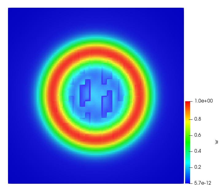 Figure 1
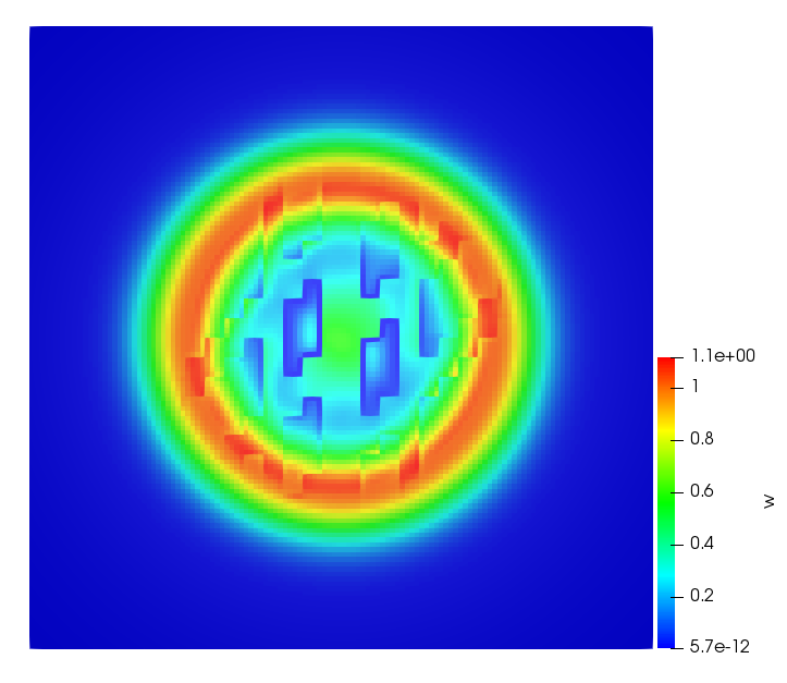 Figure 2
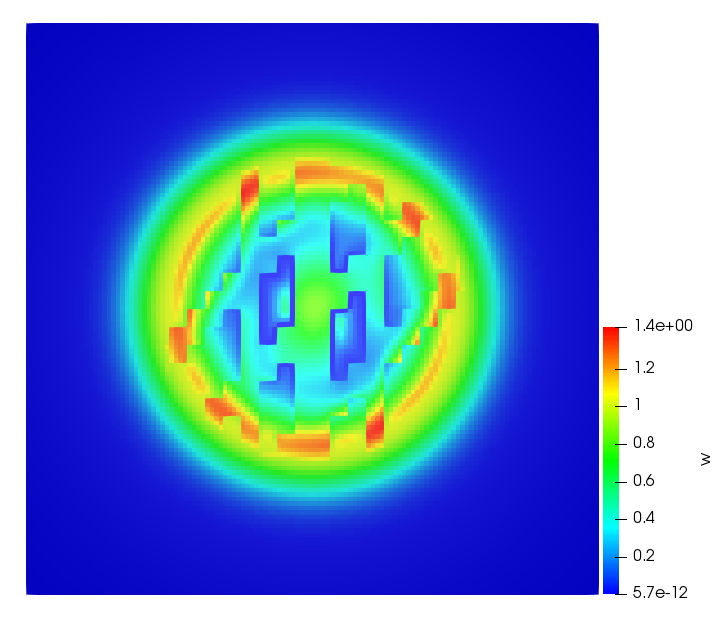 Figure 3
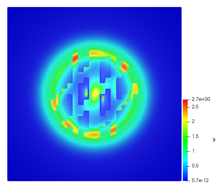 Figure 4
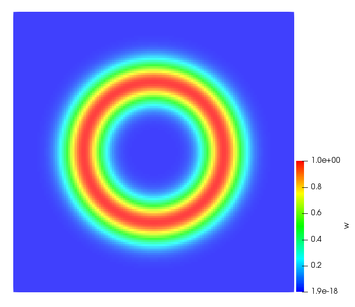 Figure 5
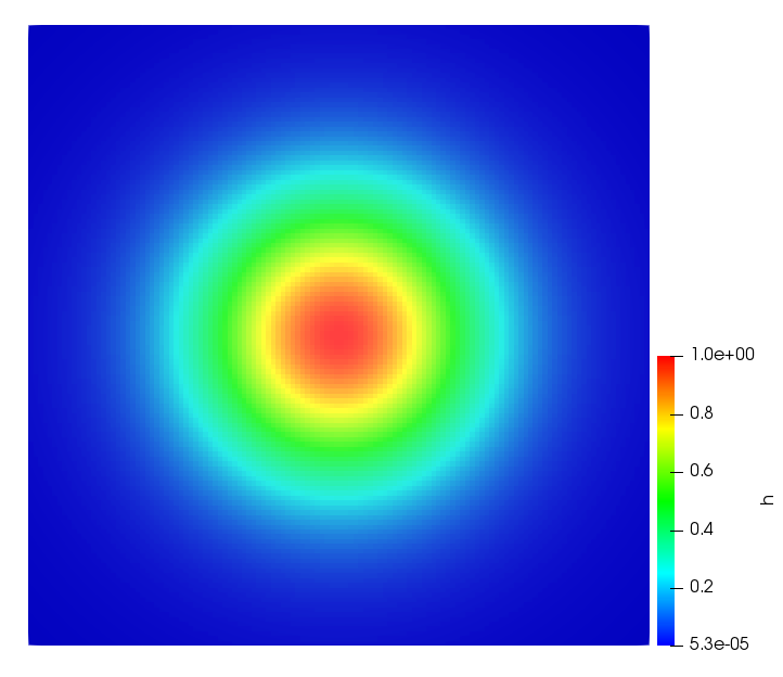 Figure 6
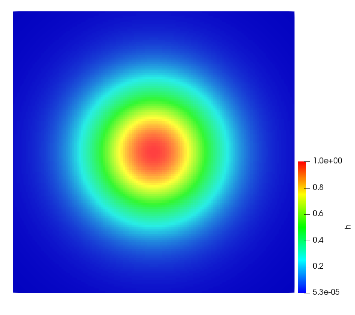 Figure 7
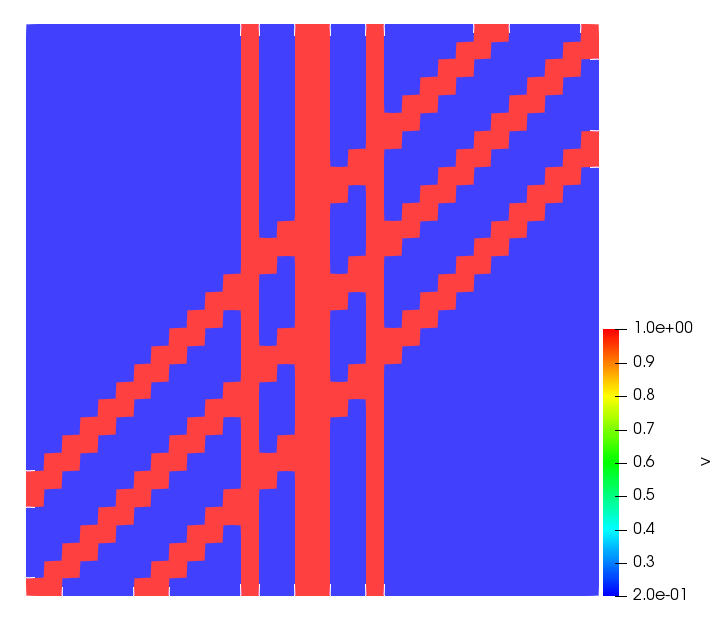 Figure 8
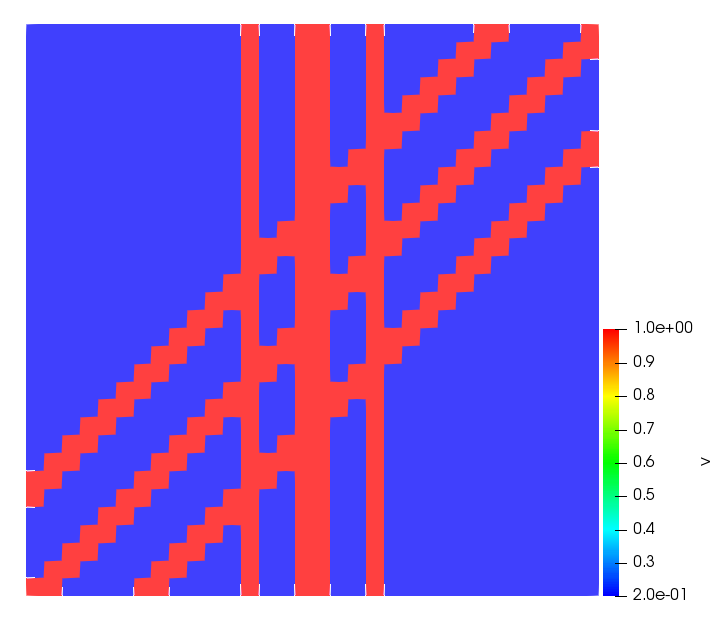 Figure 9
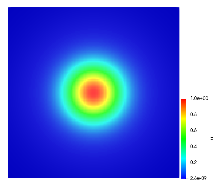 Figure 10
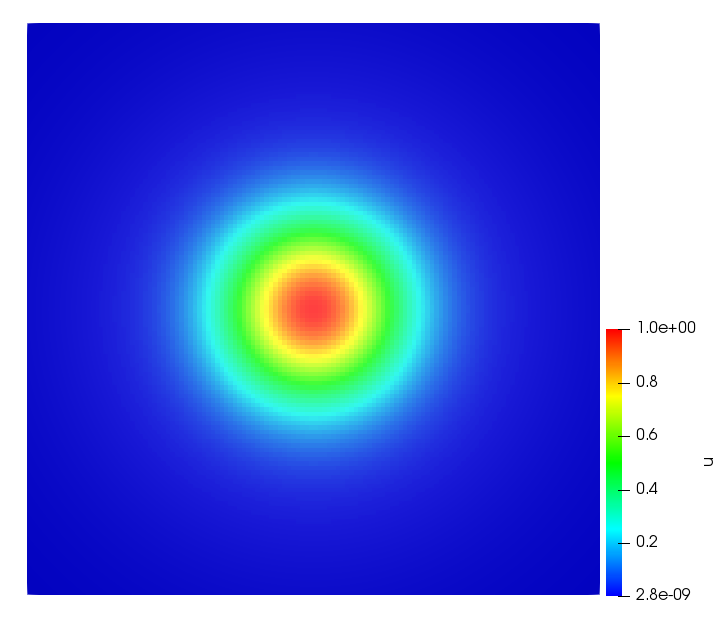 Figure 11
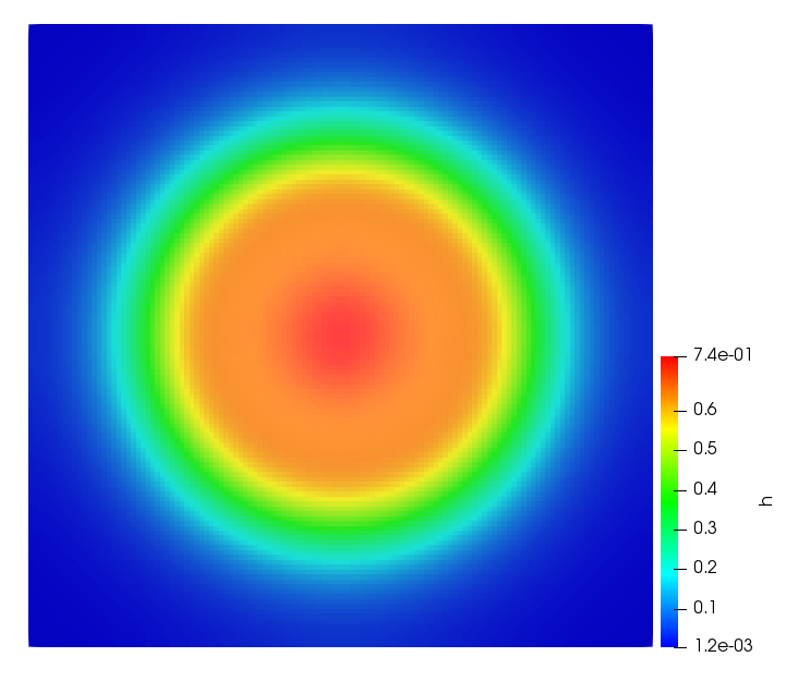 Figure 12
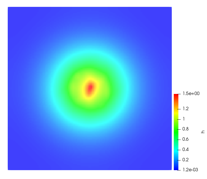 Figure 13
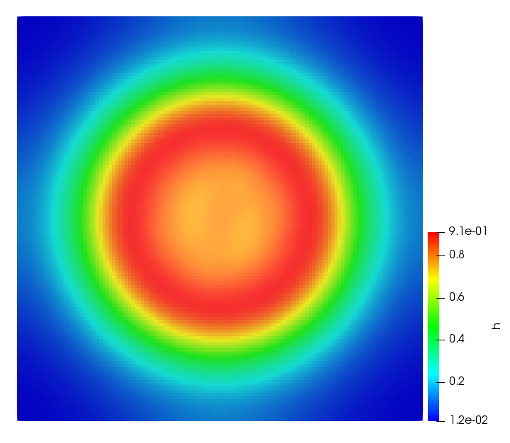 Figure 14
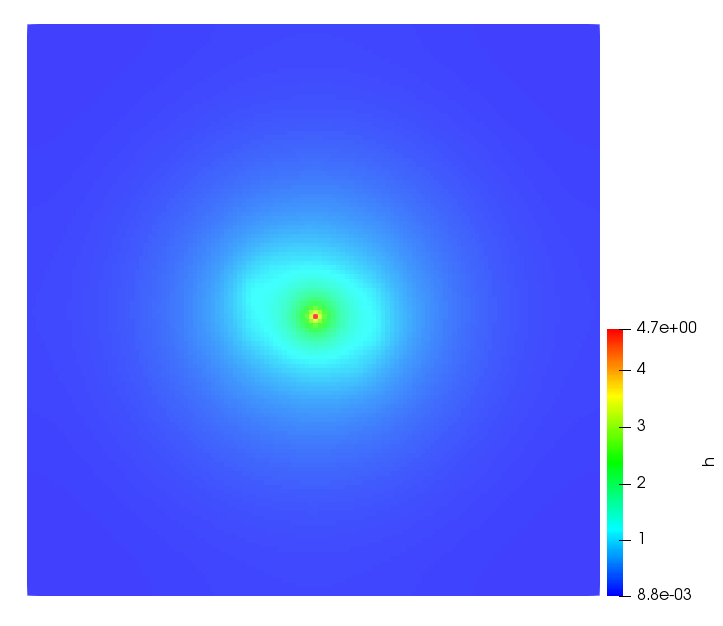 Figure 15
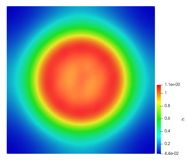 Figure 16
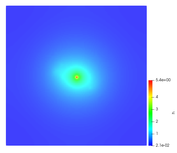 Figure 17
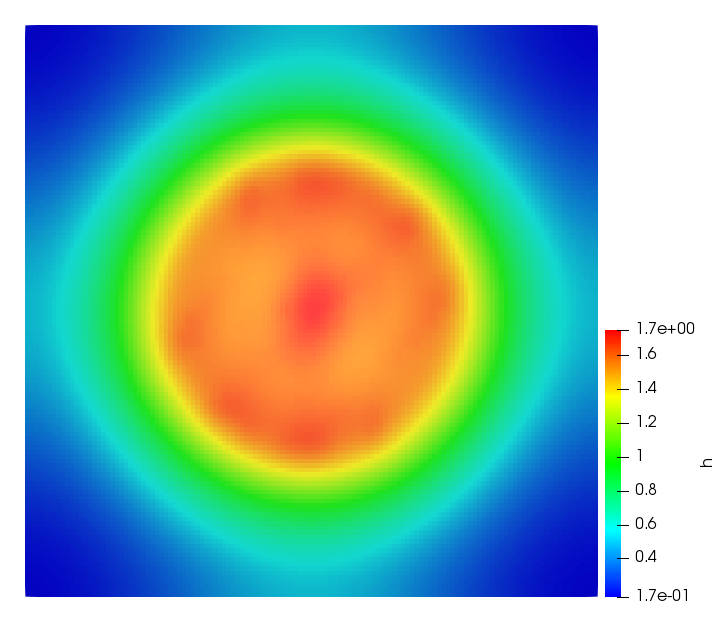 Figure 18
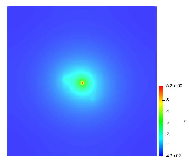 Figure 19
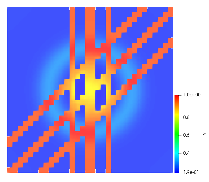 Figure 20
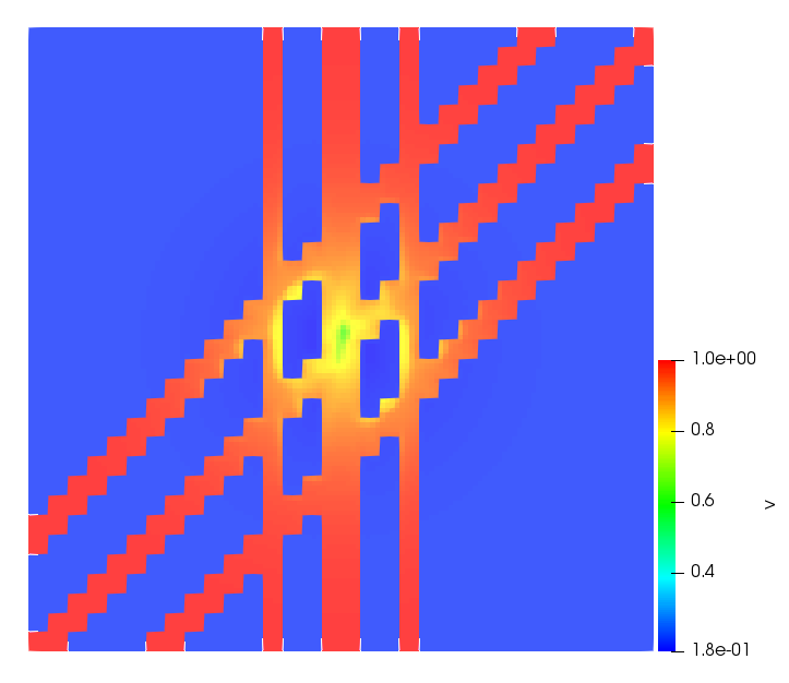 Figure 21
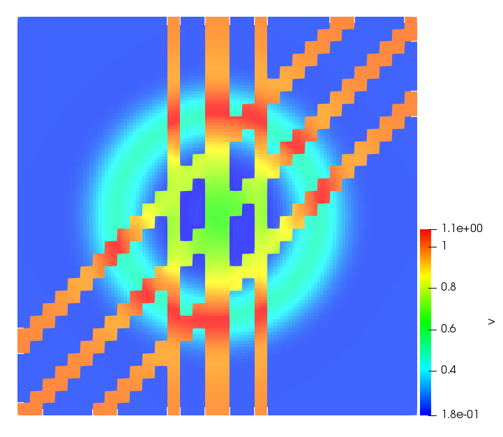 Figure 22
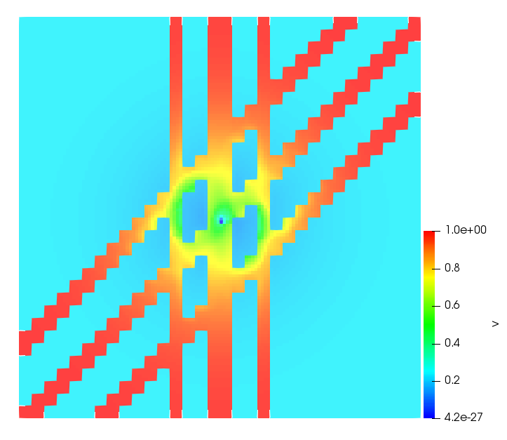 Figure 23
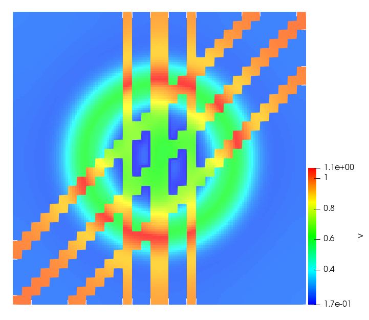 Figure 24
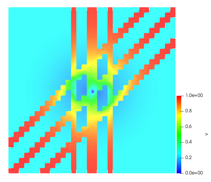 Figure 25
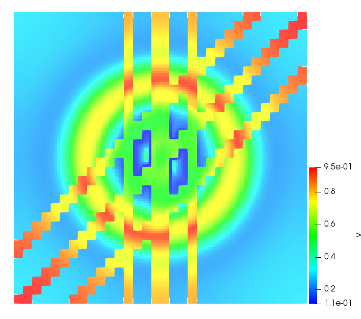 Figure 26
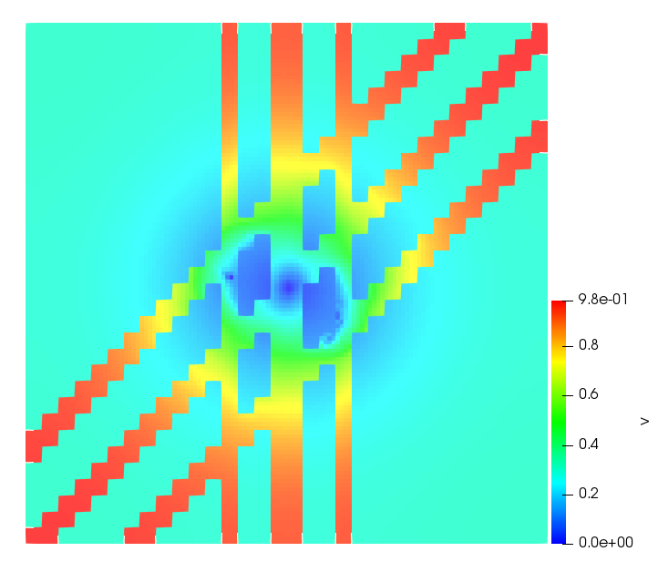 Figure 27
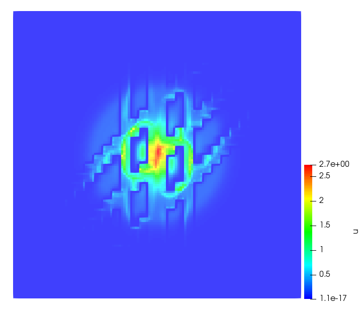 Figure 28
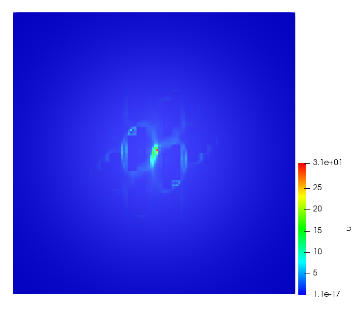 Figure 29
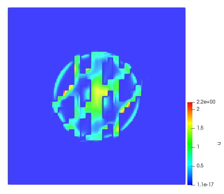 Figure 30
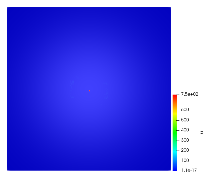 Figure 31
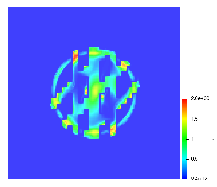 Figure 32
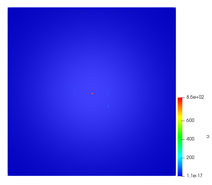 Figure 33
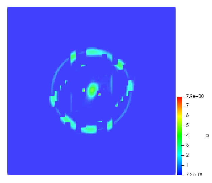 Figure 34
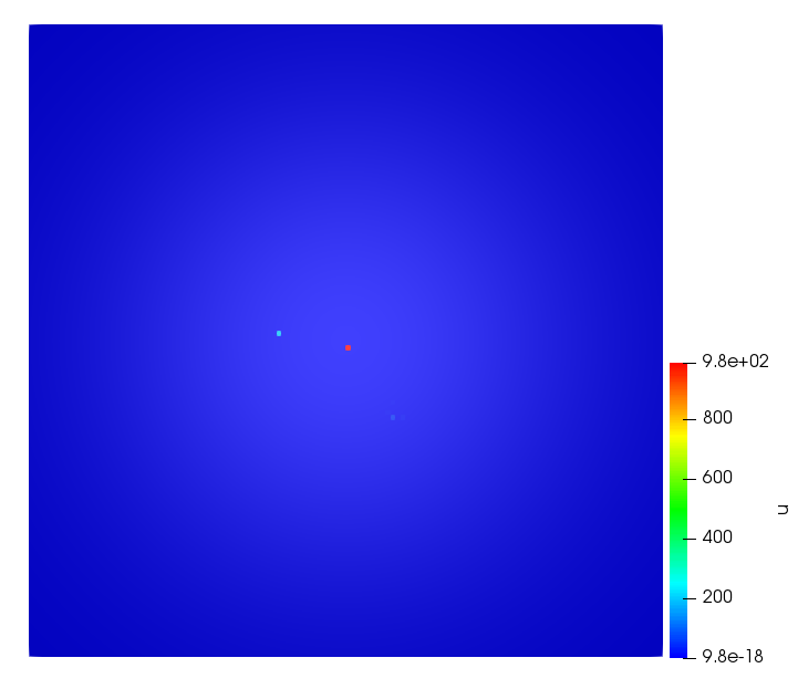 Figure 35
Peer Reviews
No public reviews on file for this paper yet. If you reviewed it on a platform where reviews are public (OpenReview, ICLR, NeurIPS, ICML), you can paste yours below so the community can read it here.
Videos
No videos yet. Explain this paper in a talk, walkthrough, or lecture? Add one.
Does indirectness of signal production reduce the explosion-supporting potential in chemotaxis-haptotaxis systems?
Global classical solvability in a class of models for cancer invasion (and more)
Christina [email protected]
Technische Universität Kaiserslautern, Felix-Klein-Zentrum für Mathematik,
67663 Kaiserslautern, Germany
Michael [email protected]
Institut für Mathematik, Universität Paderborn,
33098 Paderborn, Germany
Abstract
We propose and study a class of parabolic-ODE models involving chemotaxis and haptotaxis of a species following signals indirectly produced by another, non-motile one. The setting is motivated by cancer invasion mediated by interactions with the tumor microenvironment, but has much wider applicability, being able to comprise descriptions of biologically quite different problems. As a main mathematical feature consituting a core difference to both classical Keller-Segel chemotaxis systems and Chaplain-Lolas type chemotaxis-haptotaxis systems, the considered model accounts for certain types of indirect signal production mechanisms.
The main results assert unique global classical solvability under suitably mild assumptions on the system parameter functions in associated spatially two-dimensional initial-boundary value problems. In particular, this rigorously confirms that at least in two-dimensional settings, the considered indirectness in signal production induces a significant blow-up suppressing tendency also in taxis systems substantially more general than some particular examples for which corresponding effects have recently been observed.
Key words: chemotaxis; haptotaxis; indirect signal production; global existence
MSC: 35Q92, 35B44, 35K55, 92C17, 35A01
1 Introduction
We study here a general class of parabolic-parabolic-ODE-ODE systems (see (1.3) below) containing the following model of cancer invasion with chemotaxis and haptotaxis:
[TABLE]
supplemented with adequate initial conditions and no-flux boundary conditions. The model variables are: : density of tumor cells, : concentration of matrix metalloproteinases (MMP), : density of tissue fibers (extracellular matrix, ECM), : density of cancer associated fibroblasts (CAFs). The chemotactic bias of the cells is in the direction of the MMP gradient, while haptotaxis means as usual following the gradient of tissue density. In most of the previous chemotaxis and chemotaxis-haptotaxis models the chemoattractant is directly produced by the population performing diffusion and taxis, thereby involving ([38]) or not ([31], [43], [45]) the ECM in this production. In our present model the chemoattractant is generated in an indirect way, by the CAFs, which are activated by the tumor cells. In [5] was introduced a complex model for the evolution of a population of tumor cells interacting with two chemoattractants and also performing haptotaxis. One of the chemoattractants therein is directly produced by the cells, while the other’s production is mediated by another substance, the latter being in turn produced by the cells under the influence of the first chemoattractant. All model variables (except tissue) are diffusing in a linear way; in particular, the producers of all chemoattractants are diffusive. This is not the case in our model (1.1); moreover, both signals are completely () or partially () obtained from the non-diffusing, indirect producer .
Model (1.1) is motivated by the problem of investigating CAF-mediated cancer invasion into the surrounding tissue. CAFs are major components of the neoplasm microenvironment. They secrete a variety of extracellular matrix components and are involved in the formation of the desmoplastic stroma characterizing many advanced carcinomas ([15]). For a long time the general belief was that tumor development, invasion, and metastasis occur as a result of cancer progression. Recent studies revealed, however, that CAFs contribute instead of tumor cells to these processes, via expression of various growth factors, cytokines, chemokines, and degradation of ECM ([7], [15], [34], [36]), but also by restructuring the latter to facilitate migration ([22]). Fibronectin (Fn) assembled by CAFs mediates cell association and directional migration. Compared with normal fibroblasts, CAFs produce an Fn-rich ECM with anisotropic fiber orientation, along which the tumor cells preferentially migrate ([10]). The origin of CAFs is not completely elucidated; we refer e.g. to [6, 20] for a couple of reviews. There is evidence that they can arise among others from carcinoma cells through epithelial-mesenchymal transition (EMT) ([23]), thus allowing the cancer cells to adopt a mesenchymal phenotype associated to enhanced migratory capacity and invasiveness ([9], [30]). It has also been shown (cf. e.g. [29]) that cancer cells can reprogram resident tissue fibroblasts to become CAFs through the actions of miRNAs. MMPs are primarily derived from CAFs in various types of tumor ([23], [26], [42]). In particular, it has been shown e.g., that MMP-9, an endoproteinase involved in ECM degradation and implicated as a prerequisite of metastasis, has very limited or no expression in various cancer cell lines. Instead, MMP-9 is well-known to be secreted from cancer stromal fibroblasts and endothelial cells ([39]). For further information about CAFs and their MMP production we refer, e.g., to the review [26]. The main features of CAF-mediated tumor invasion mentioned above are captured in our model (1.1) below.
Closely related from a mathematical viewpoint is the chemotaxis-haptotaxis model
[TABLE]
which describes the evolution of two cancer cell subpopulations either proliferating () or migrating (), with the corresponding transitions between the two phenotypes, and in interaction with tissue () and acidity (). The latter is mainly produced by the highly glycolytic proliferating tumor cells – hence indirect signal production. The proliferation/migration (also known as go-or-grow) dichotomy asserting that moving cells defer their proliferation seems to be a relevant feature for some types of cancer ([13], [21],[49]) and can lead to interesting mathematical problems and qualitative behavior of the corresponding heterogeneous tumor ([37], [51]). The migrating cells in (1.2) perform haptotaxis and pH-taxis: they move towards increasing ECM gradient and away from acidic (thus hypoxic) areas. The conversion from proliferating to migrating cells depends on the concentration of protons in the peritumoral region and infers limitations, as only a rather small part of the tumor becomes motile -usually cells situated at the tumor margins. Moreover, the protons are buffered by the environment (e.g., uptake by vasculature), contribute to tissue degradation, and restrict tumor proliferation. Supplementary to hypoxia the tissue can be degraded by chemical or biological agents directly or indirectly produced or activated by the tumor cells, see e.g. [27] and [28]. The ECM remodeling also involves limited, logistic-like growth. The latter is also used in (1.2) to describe tumor cell proliferation. We note here that taking squares of the positive parts of the proliferation terms is motivated by the mainly technical need of satisfying the regularity assumptions in Theorem 1.1 and could perhaps be relaxed; in fact, the difference between functions of this type just involving the positive parts and those taking their squares is rather small. System (1.2) fits in the theoretical framework proposed and analyzed below.
Thus the general model class to be introduced and studied here includes descriptions of biologically quite different problems, as exemplified above. It therefore provides a comprehensive mathematical structure for several issues related to cancer cell migration under the influence of chemo- and haptotactic effects, including some variants of the often addressed Chaplain-Lolas model from [5]. Other problems characterizing tactic cell migration, e.g. in wound healing and/or angiogenesis or interacting microbial populations in biofilm formation and persistence, can potentially be cast into this mathematical framework. Models describing the dynamics of a species performing chemotaxis towards the gradient of a signal produced by another, non-tactic species (see e.g. [19] and [47]) form a subclass of this setting.
Approaching a mathematical core feature: indirectness of chemoattractant production. From a purely mathematical perspective, a common feature distinguishing both (1.2) and (1.1) from classical chemotaxis or chemotaxis-haptotaxis systems of Keller-Segel or Chaplain-Lolas type consists in the circumstance that the respective mechanisms of chemoattractant production are indirect in the sense that the corresponding signal is not produced directly by individuals of the cell population, but rather through a third agent. Possible implications on the system dynamics, however, have apparently been detected only in some quite particular examples of chemotaxis-only models: Indeed, the only findings in this direction we are aware of concentrate on associated derivates of the classical Keller-Segel system, for which substantial blow-up preventing effects of such indirect signal production mechanisms have recently been revealed. More precisely, in sharp contrast to what is known for standard Keller-Segel systems ([17], [2]), regardless of the size of the initial data some corresponding spatially two-dimensional initial-boundary value problems always possess globally defined classical solutions ([47], [25]).
Complementary to its biological motivation, the main mathematical purpose of the present work is to rigorously confirm that such relaxing effects of indirect chemoattractant production are actually not restricted to cases of chemotaxis-only systems, but rather seem to form a much more general and robust feature of chemotactic interaction also in significantly more contexts involving haptotactic migration mechanisms with all their potentially regularity-limiting properties due to lack of haptoattractant diffusion.
This will subsequently be examined in the framework of the problem
[TABLE]
in a bounded domain with smooth boundary, where the parameters , , and are assumed to be positive, and where for simplicity we suppose throughout this paper that with some ,
[TABLE]
As for the parameter functions in (1.3), in order to create a setup sufficiently general so as to include both (1.2) and (1.1), we shall require that
[TABLE]
and are such that
[TABLE]
and
[TABLE]
that
[TABLE]
and that
[TABLE]
and finally
[TABLE]
As can readily be verified, indeed both models (1.2) and (1.1) then become special cases of the PDE system in (1.3) whenever the parameters and therein are positive, whereas for and and, in particular, is merely required to be nonnegative.
Our main results in this context then read as follows.
Theorem 1.1
Let be a bounded domain with smooth boundary, assume that and are positive, and suppose that , , , and satisfy (1.5), (1.6), (1.7), (1.8), (1.9) and (1.10). Then for any choice of fulfilling (1.4) with some , the problem (1.3) possesses a uniquely determined globally defined classical solution for which and are nonnegative.
In particular, Theorem 1.1 asserts that indeed no finite-time blow-up occurs in (1.3) under the above assumptions, and that in this regard the solution behavior in (1.3) quite drastically differs from that in the corresponding variants of (1.2) and (1.1) in which the second equation is replaced with e.g. , and in which already in the semi-trivial case when , known results on the actually resulting two-component Keller-Segel system for assert finite-time blow-up for some solutions ([16]).
In line with this, all known results even on global existence, but also on qualitative properties, in the original Chaplain-Lolas model ([5])
[TABLE]
seem to strongly rely on the assumption that be positive, thus guaranteeing the presence of a logistic-type quadratic growth restriction on the cell density ([4], [32], [31], [40], [41], [46], [48]). Our results show that in the context of the variant (1.1) of (1.11) involving indirect chemoattractant production, no such additional dampening is necessary: Indeed, even when tissue remodeling is included by supposing that in (1.1), Theorem 1.1 asserts global classical solvability in (1.1) for actually any nonnegative value of .
The paper is structured as follows: After stating a result on local existence and extensibility as well as some preliminary estimates in Section 2, in Section 3 we shall construct a quasi-energy functional for (1.3) and draw some immediate conclusions concerning regularity of solutions. The accordingly obtained estimates are used as a starting point for a Moser-type iterative argument yielding bounds for the key solution component in Section 4, and hence paving an essential part of the way toward our proof of Theorem 1.1 in Section 5. Finally, in Section 6 we illustrate the theoretical findings by numerical simulations of (1.1) and the corresponding model with direct signal production and provide some comments about the obtained results.
2 Local existence and basic estimates
Following several precedents in the literature ([11], [12], [31]), in order to establish a preliminary result on local existence, but also to prepare our subsequent estimation procedure, we note that on substituting
[TABLE]
the problem (1.3) is equivalently transformed to
[TABLE]
In this formulation, with respect to the construction of local-in-time solutions the problem (1.3) indeed becomes accessible to appropriate fixed point frameworks; by straightforward and minor adaptations of the corresponding arguments detailed e.g. in [31], it is thereby possible to establish the following basic statement on unique solvability and extensibility.
Lemma 2.1
Let and be positive, let , , , and comply with (1.5), (1.6), (1.7), (1.8), (1.9) and (1.10), and suppose that satisfies (1.4) with some . Then there exist and a uniquely determined classical solution of (2.2) such that
[TABLE]
Moreover, we have and in .
Without any further explicit mentioning, throughout the sequel we shall suppose that the assumptions of Lemma 2.1 are satisfied, and that and are as provided by the latter. Moreover, we shall tactitly switch between these variables and the quadruple solving (1.3) classically in , as thereby defined through (2.1).
A first boundedness property of this solution is immediate.
Lemma 2.2
The solution of (1.3) satisfies
[TABLE]
Proof. As from (1.3), (1.8) and (1.9) we know that
[TABLE]
by means of a simple comparison argument we conclude that
[TABLE]
Herein estimating for , from this we readily obtain (2.4). Next, thanks to (1.6) and (1.7) the first and fourth solution components in (1.3) can at least controlled with respect to their norm in in a fairly simple manner.
Lemma 2.3
Let . Then there exists such that
[TABLE]
as well as
[TABLE]
where .
Proof. Using that v\leq c_{1}(T):=\Big{\{}\|v_{0}\|_{L^{\infty}(\Omega)}+\frac{C_{\Phi}}{C_{\phi}}\Big{\}}\cdot e^{C_{\phi}T} in due to Lemma 2.2, after spatial integration in the first and the fourth equation in (1.3) and adding the respective results we may rely on (1.6) and (1.10) in estimating
[TABLE]
for . A time integration of this linear ODI for directly yields (2.5). Similarly, (1.7) implies that
[TABLE]
for all , so that (2.6) becomes a consequence of (2.5).
3 A quasi-energy inequality
The purpose of this section consists in the construction of an Lyapunov-like functional which through a corresponding energy-dissipation inequality will provide some fundamental regularity information that will form the starting point of a series of a priori estimates which in the presently considered spatially two-dimensional setting will finally allow for the conclusion that is actually global in time.
As our first step in this direction, let us perform a standard testing procedure by which the crucial haptotactic contribution to the first equation in (1.3) is reduced to an inner product of gradients:
Lemma 3.1
Let . Then
[TABLE]
for all .
Proof. In the identity
[TABLE]
valid for all due to (1.3), we use Young’s inequality to estimate
[TABLE]
Moreover, by means of (1.6) we see that for all ,
[TABLE]
and
[TABLE]
because for all . In conjunction with (3.2)-(3.4), this establishes (3.1). Now in order to achieve a precise cancelation of the integral in (3.1) stemming from haptotactic cross-diffusion, inspired by several precedent works on similar types of interaction (see e.g. [8], [45] and [38]), we track the evolution of the Dirichlet integral associated with .
Lemma 3.2
The solution of (1.3) has the property that
[TABLE]
Proof. According to the third equation in (1.3), we have
[TABLE]
Here from (1.8) we know that
[TABLE]
and that due to Young’s inequality, for all we have
[TABLE]
and
[TABLE]
as well as
[TABLE]
and
[TABLE]
Moreover, combining Young’s inequality with (1.9) we can estimate
[TABLE]
As the second summand on the right of (3.7) is nonpositive, collecting (3.8)-(3.13) we thus infer (3.5) from (3.7). Next, several expressions on the right-hand sides of (3.1) and (3.5) need to be controlled in modulus. Here the second integral on the right of (3.1) can in fact be absorbed by the dissipation rate appearing in the following inequality gained by means of a standard procedure.
Lemma 3.3
For all ,
[TABLE]
Proof. On testing the second equation in (1.3) by and using Young’s inequality in a standard manner, we obtain
[TABLE]
which implies (3.14) due to the fact that by (1.7) and again Young’s inequality,
[TABLE]
in . The second last summand in (3.5), referring to the component with evolution governed by an ODE only, apparently cannot be expected to be absorbed by some suitable dissipation rate. The following lemma indicates that at least some exponential control thereof will eventually be possible.
Lemma 3.4
We have
[TABLE]
Proof. Using the fourth equation in (1.3), we compute
[TABLE]
where by Young’s inequality,
[TABLE]
and where by (1.10),
[TABLE]
Apart from that, combining (1.10) with Young’s inequality we see that
[TABLE]
and
[TABLE]
as well as
[TABLE]
and
[TABLE]
for all . Inserting (3.17)-(3.22) into (3.16) directly yields (3.15). A final minor ingredient to our quasi-energy inequality is addressed in the following.
Lemma 3.5
If , then
[TABLE]
Proof. As
[TABLE]
by (1.3), this follows by observing that
[TABLE]
due to Young’s inequality, and that
[TABLE]
according to (1.10). As a last preparation, let us make use of appropriate parabolic regularization features to estimate terms of the form appearing in the last integral from (3.15).
Lemma 3.6
Let . Then there exists with the property that for all one can find such that
[TABLE]
where again .
Proof. We first note that according to (1.7), Lemma 2.2 and Lemma 2.3 we can fix positive constants and such that
[TABLE]
and that
[TABLE]
and observe that since it is possible to choose suitably close to satisfying . In the Duhamel representation
[TABLE]
we may then use standard - estimates for the Neumann heat semigroup ([50, Lemma 1.3]) to find such that for all ,
[TABLE]
As (3.25) and (3.26) warrant that
[TABLE]
this readily entails that
[TABLE]
with being finite due to our restriction . Now since a combination of the Gagliardo-Nirenberg inequality with elliptic regularity theory yields such that
[TABLE]
from (3.27) we immediately obtain (3.24) with fulfilling according to the inequality . We can now proceed to our detection of an energy-like structure in (1.3), as expressed in the following lemma.
Lemma 3.7
Let . Then there exist and such that for
[TABLE]
and
[TABLE]
we have
[TABLE]
where .
Proof. Thanks to Lemma 2.3 and Lemma 2.2, we can fix positive constants and such that
[TABLE]
as well as
[TABLE]
Then in accordance with the Gagliardo-Nirenberg inequality, choosing such that
[TABLE]
we define
[TABLE]
and take large enough fulfilling
[TABLE]
Finally picking small such that both
[TABLE]
and
[TABLE]
hold, we let and be as determined through (3.28) and (3.29) and claim that then (3.30) is valid with some suitably large .
To this end, we first take an appropriate linear combination of the inequalities provided by Lemma 3.1, Lemma 3.3, Lemma 3.2, Lemma 3.4 and Lemma 3.5, which when applied to our particular value of namely show that
[TABLE]
[TABLE]
with obvious definitions of for , where we have made use of a favorable cancelation in some contributions stemming from the haptotactic interaction.
Now employing (3.33) we see that due to (3.31) and (3.34) we have
[TABLE]
whereas Lemma 3.6 says that as , there exist and such that
[TABLE]
whence by Young’s inequality,
[TABLE]
with some . Since moreover the Poincaré inequality provides satisfying
[TABLE]
thanks to the restrictions in (3.35), (3.36) and (3.37) we conclude from (3.38), (3.39) and (3.40) that there exists such that
[TABLE]
for all . Using that for all and thus for all , from this we finally obtain that for all ,
[TABLE]
as intended. Upon integration, the latter implies several a priori estimates, significantly going beyond those from Lemma 2.2 and Lemma 2.3, among which we explicitly state only those three inequalities that will be referred to later on.
Lemma 3.8
For all there exists such that again writing we have
[TABLE]
and
[TABLE]
as well as
[TABLE]
Proof. Upon integrating (3.30) in time, we can find such that with and taken from (3.28) and (3.29) we have
[TABLE]
Once more using that for , from this we readily obtain the claimed inequalities as particular consequences. As an immediate consequence, let us add the following observation about regularity of .
Corollary 3.9
Let and . Then there exists such that with ,
[TABLE]
Proof. As , combining (2.6) with (3.42) immediately yields (3.44).
4 bounds for
In this section we intend to make use of the information from Lemma 3.8 in order to finally achieve an a priori bound for the quantity from (2.1), and hence for , with respect to the norm in . Here a key role will be played by the following implication of the estimate (3.41) on a Gagliardo-Nirenberg-type interpolation, as expressed in the following.
Lemma 4.1
Let and . Then for all one can find such that
[TABLE]
with .
Proof. This follows in a standard manner from the boundedness property of in as implied by Lemma 3.8 and Lemma 2.2, by means of a refined interpolation inequality of Gagliardo-Nirenberg type, the latter going back to [3] and extended to a version applicable to the present setting in [45, Lemma A.5] (for details, see e.g. [45, p.800]). In order to make appropriate use of this, let us perform another well-established testing procedure to (2.2), a basic outcome of which is the following.
Lemma 4.2
Let . Then there exists such that for all and all with ,
[TABLE]
Proof. By means of (2.2), we obtain
[TABLE]
for all , where by Young’s inequality,
[TABLE]
for all , with being finite according to Lemma 2.2. Furthermore, (1.6) and Young’s inequality warrant that for all ,
[TABLE]
while from (1.8) and (1.9) we know that
[TABLE]
and that
[TABLE]
As clearly , by nonnegativity of we therefore infer (4.2) from (4.3) when combined with (4.4), (4.5), (4.6) and (4.7). Here a suitable control of the crucial rightmost summand in (4.2) will rely, besides on Lemma 4.1, also on the following statement which can be viewed as partially generalizing Lemma 3.5.
Lemma 4.3
Let and . Then writing and , with some we have
[TABLE]
Proof. Choosing large enough fulfilling in according to Lemma 2.2, equation (1.3), and due to Young’s inequality and (1.10) we can estimate
[TABLE]
so that with some we have
[TABLE]
An integration thereof shows that
[TABLE]
and hence implies (4.8). We can thereby use Lemma 4.2 along with Lemma 4.1 to derive the following estimate for , at this stage yet involving bounds possibly depending on the finite number .
Lemma 4.4
Let and . Then there exists such that
[TABLE]
where again .
Proof. From Lemma 4.2 we obtain and such that
[TABLE]
again because . Here since Lemma 3.8 provides such that
[TABLE]
by means of Young’s inequality and the Gagliardo-Nirenberg inequality we infer that with some we have
[TABLE]
Therefore, (4.10) shows that there exists such that , , satisfies
[TABLE]
for all and thus, upon integration,
[TABLE]
for all , where again we have set . As thus is positive, a well-known result on maximal Sobolev regularity in the parabolic subproblem of (1.3) satisfied by ([14]) becomes applicable so as to yield satisfying
[TABLE]
for all because of (1.7). Since Corollary 3.9 and Lemma 4.3 provide and such that
[TABLE]
and that
[TABLE]
this means that with some we have
[TABLE]
so that from (4.12) we infer the existence of satisfying
[TABLE]
We now employ Lemma 4.1 to see that with some ,
[TABLE]
whence (4.13) ensures that
[TABLE]
and that thus, clearly, (4.9) holds. By adapting a well-established Moser-type iteration ([1], [44]) to the present context, however, one can readily turn the latter into estimates in .
Lemma 4.5
Given , one can find such that with we have
[TABLE]
Proof. We first fix any and then obtain upon combining Lemma 4.4 with Lemma 4.3, Lemma 2.2, (1.7) and Corollary 3.9 that
[TABLE]
with and some . As a consequence thereof, standard regularization features of the Neumann heat semigroup ([50, Lemma 1.3], [18, Lemma 4.1]) entail boundedness of in , so that from Lemma 4.2 we infer the existence of and such that for and any nonnegative integer ,
[TABLE]
On integrating and recalling Lemma 2.2 and Lemma 4.3, we see that with some , for any such and arbitrary we have
[TABLE]
The remaining part now follows a well-established reasoning: According to the Gagliardo-Nirenberg inequality and Young’s inequality, we can find such that introducing the numbers
[TABLE]
all finite due to Lemma 4.4, for and each we have
[TABLE]
whence (4.15) entails that for some ,
[TABLE]
By means of a standard recursive argument, both when for infinitely many , and as well in the opposite case this can readily be seen to imply the existence of such that
[TABLE]
from which the claim immediately follows.
5 Global extensibility. Proof of Theorem 1.1
Having thus ruled out blow-up of the first quantity appearing in the second alternative from (2.3), it hence remains to derive appropriate bounds for the haptotactic gradient. A first observation relates the latter to some spatio-temporal regularity properties of and .
Lemma 5.1
Let and . Then there exists fulfilling
[TABLE]
for all , with and .
Proof. Differentiating in (1.3) and recalling (2.1), we see that throughout ,
[TABLE]
and
[TABLE]
where we have suppressed the argument in , and the derivatives thereof. Now as a consequence of Lemma 2.2, Lemma 4.5 and (2.1), our requirements (1.8), (1.9) and (1.10) guarantee that herein all the functions , , , , , , and are bounded in , so that (5.2) and (5.3) imply that with some we have
[TABLE]
and, similarly,
[TABLE]
for all . Adding these inequalities and invoking Gronwall’s lemma readily leads to (5.1). Here the crucial ingredient containing will ultimately be controlled by using the following result which extends a corresponding statement from [45, Lemma 3.14] to the present more complex system (2.2).
Lemma 5.2
Let . Then there exists with the property that
[TABLE]
where again and .
Proof. Defining
[TABLE]
for , we see that the first equation in (2.2) simplifies to the identity
[TABLE]
which we multiply by and integrate to find using Young’s inequality that for all and any ,
[TABLE]
Here we note that given , in view of the boundedness property of in asserted by Lemma 4.5 we can fix such that due to Young’s inequality,
[TABLE]
Moreover, as the Gagliardo-Nirenberg inequality together with elliptic estimates and Lemma 4.5 provides and such that
[TABLE]
by combining the Cauchy-Schwarz inequality with Young’s inequality we obtain
[TABLE]
which along with (5.6) shows that (5.5) implies the inequality
[TABLE]
with some appropriately large .
To proceed from this, we observe that as a consequence of Lemma 5.1 we can find such that
[TABLE]
and that another application of the Gagliardo-Nirenberg inequality in conjunction with Lemma 3.8 provides and fulfilling
[TABLE]
Therefore, again through Lemma 3.8, (5.8) reduces to
[TABLE]
where by the Fubini theorem and, again, (5.7),
[TABLE]
We now let be small enough such that , and choose and such that and for all . Then inserting (5.10) into (5.9) shows that
[TABLE]
along with and satisfy
[TABLE]
whence if we let
[TABLE]
then
[TABLE]
with . Therefore, for all , which in view of the definitions of and yields (5.4). Combining this with Lemma 5.1 readily implies the following.
Lemma 5.3
For all and one can fix such that with and we have
[TABLE]
Proof. From Lemma 5.2 in conjunction with elliptic regularity theory we obtain such that
[TABLE]
which we combine with the continuity of the embedding and the Cauchy-Schwarz inequality to conclude that with some we have
[TABLE]
Since Lemma 3.8 in quite a similar fashion yields the existence of such that
[TABLE]
the claimed estimate is a consequence of Lemma 5.1. Now our main result has actually already been established:
Proof of Theorem 1.1. Thanks to Lemma 2.1, and in particular the extensibility criterion (2.3) therein, we only need to combine the outcome of Lemma 4.5 with an application of Lemma 5.3 to .
6 Simulations and discussion
To illustrate our theoretical results we also performed some numerical simulations of the version
[TABLE]
of the indirect signal production model (1.1) and – for comparison purposes – we also simulated some solutions of the system
[TABLE]
in which the signal (MDEs) is directly produced by the tumor cells. Since for both models there is no blow-up as long as (see [24] for the result concerning (6.13)), we only considered here the case with no tumor cell proliferation, i.e. .
The simulations were performed using a discontinuous Galerkin FEM method. Thereby, the diffusion was discretized in space by using a symmetric interior penalty Galerkin (SIPG) method (see [35]), while for the drift term we did an upwind discretization. The time was discretized with an IMEX procedure handling the diffusion implicitly and the reaction and taxis terms explicitly. The computational domain was and the initial conditions for tumor cells and MDEs were chosen in the form , , with , . For the initial density of CAFs we considered a radially symetric form with and . Finally, the initial tissue density was characterized by v_{0}(x)=\left\{\begin{array}[]{cc}v_{\text{max}},&x\in\Omega_{v}\\ v_{\text{min}},&x\not\in\Omega_{v}\end{array}\right., with and , thus representing the stripes shown in the second columns of Figures 1 and 2. Together these initial conditions describe a heterogeneous tissue structure, in which a Gaussian-shaped tumor is embedded, surrrounded by activated CAFs and featuring higher MDE concentration in the areas with many tumor cells. We considered for both models (where applicable) the following parameters: ; ; ; ; ; ; ; . The results are shown in Figure 1 for system (6.12) and in Figure 2 for system (6.13). The first rows represent the initial conditions, and the subsequent rows illustrate the solution behavior at several successive time steps.
The simulations of (6.12) depicture an increase in tumor cell density, which is, however, limited. Same applies to the MDE concentration and CAFs density, but with smaller rates. The tissue is correspondingly degraded, and the CAFs spread into the region containing the main tumor mass, at the same time building up some tissue (for a sufficiently large , as in these simulations) at the sites where they are abundant enough. In contrast, model (6.13) predicts localized tumor cell aggregates of very high density which are almost three orders of magnitude higher than the initial condition and keep growing in time, thus hinting on blow-up of the solution. Likewise, in this latter setting the MDE concentration is directly produced by the tumor cells and keeps growing as well, although to a much smaller rate than the cell density. The tissue degradation is much more localized and – where it happens – stronger. These results are conform with the theoretical findings in this and previous papers predicting blow-up of solutions when the signal was directly produced by the agents performing chemotaxis ([2]), while the solutions stay bounded in the case of indirect signal production.
From a biological viewpoint the tumor cells use CAFs (which are originally ’harmless’ stroma cells only becoming supporters of tumor invasion upon activation) to produce matrix degrading factors. As mentioned above, the production of the latter seems to be decisively controled by CAFs, hence is rather indirect, as the neoplastic cells first need to activate the CAFs, which then enhance degradation of surrounding tissue and cell motility, including chemotaxis towards the gradient of proteolytic agents. Our mathematical result actually tells that such mediation of invasion leads to avoidance of blow-up, unlike previous models where the direct production of chemoattractant let the solution(s) become unbounded, a rather unrealistic biological scenario. The result is in line with many in vivo and in vitro observations that cancer cells ’hijack’ their environment in order to gain migratory, survival, and proliferative advantages.
We considered here that CAFs were non-diffusing, although they are indeed able to spread [42]. Accounting for diffusion of the chemoattractant producer does not pose, however, any further challenge to the analysis of our model (1.1); in that case our setting belongs to the same mathematical class as the one in [5], to which it is also biologically related: both describe the evolution of a tumor under chemotaxis and haptotaxis, the chemoattractant(s) – of which MDEs are considered in both models – being supposed to diffuse.
Further chemotaxis-haptotaxis models belonging to the class studied here can be considered, of which (1.2) is just one example. As mentioned above, a diffusing signal producer can be easily accomodated to this model class – if the diffusion is linear. Solution-dependent diffusions of either involved species need further investigation; in [33] one such system extending that from [47] to allow for nonlinear diffusion of the chemotactic species has been studied, however without haptotaxis.
Acknowledgement
The authors thank Aydar Uatay (TU Kaiserslautern) for performing the numerical simulations. The second author acknowledges support by Deutsche Forschungsgemeinschaft in the framework of the project Emergence of structures and advantages in cross-diffusion systems (No. 411007140, GZ: WI 3707/5-1).
The reference list from the paper itself. Each links out to its DOI / PubMed record.
- 1[1] Alikakos, N.D.: L p superscript 𝐿 𝑝 L^{p} bounds of solutions of reaction-diffusion equations. Comm. Part. Differential Eq. 4 , 827-868 (1979)
- 2[2] Bellomo, N., Bellouquid, A., Tao, Y., Winkler, M.: Toward a mathematical theory of Keller-Segel models of pattern formation in biological tissues. Math. Models Methods Appl. Sci. 25 , 1663-1763 (2015)
- 3[3] Biler, P., Hebisch, W., Nadzieja, T.: The Debye system: Existence and large time behavior of solutions. Nonlinear Analysis 23 (9), 1189-1209 (1994)
- 4[4] Cao, X.: Boundedness in a three-dimensional chemotaxis-haptotaxis system. Z. Angew. Math. Phys. 67 , 11 (2016)
- 5[5] Chaplain, M.A.J., Lolas, G.: Mathematical modelling of cancer invasion of tissue: The role of the urokinase plasminogen activation system. Math. Models Methods Appl. Sci. 15 , 1685-1734 (2005).
- 6[6] Cirri, P., Chiarugi, P.: Cancer associated fibroblasts: the dark side of the coin. Am. J. Cancer Res. 1 , 482-497 (2011).
- 7[7] Cirri, P., Chiarugi, P.: Cancer associated fibroblasts and tumour cells: A diabolic liaison driving cancer progression. Cancer Metast. Rev. 31 , 195-208 (2012).
- 8[8] Corrias, L., Perthame, B., Zaag, H.: Global solutions of some chemotaxis and angiogenesis systems in high space dimensions. Milan J. Math. 72 , 1-28 (2004)