A physicist's guide to explicit summation formulas involving zeros of Bessel functions and related spectral sums
Denis S. Grebenkov

TL;DR
This paper reviews methods for explicitly computing spectral sums involving Bessel function zeros, crucial for various diffusion-related applications, emphasizing practical strategies and their limitations.
Contribution
It provides a comprehensive pedagogic overview of analytical tools and summation formulas for spectral sums involving Bessel function zeros, with practical insights.
Findings
Summarizes three main strategies for spectral sum computation.
Highlights advantages and limitations of each method.
Provides a collection of summation formulas from literature.
Abstract
We summarize the mathematical basis and practical hints for the explicit analytical computation of spectral sums that involve the eigenvalues of the Laplace operator in simple domains. Such spectral sums appear as spectral expansions of heat kernels, survival probabilities, first-passage time densities, and reaction rates in many diffusion-oriented applications. As the eigenvalues are determined by zeros of an appropriate linear combination of a Bessel function and its derivative, there are powerful analytical tools for computing such spectral sums. We discuss three main strategies: representations of meromorphic functions as sums of partial fractions, Fourier-Bessel and Dini series, and direct evaluation of the Laplace-transformed heat kernels. The major emphasis is put on a pedagogic introduction, the practical aspects of these strategies, their advantages and limitations. The review…
Click any figure to enlarge with its caption.
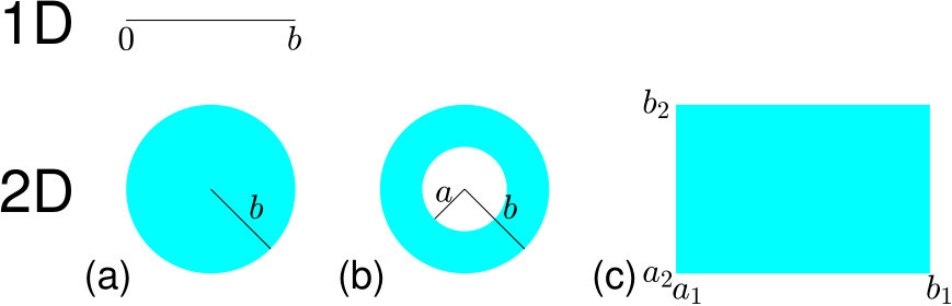 Figure 1
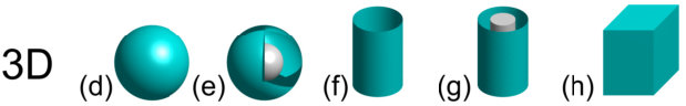 Figure 1
| Disk | Ball | |
|---|---|---|
| Domain | ||
| Coordinates | Polar | Spherical |
| Laplacian | ||
| eigenfunctions | ||
| indices | , | |
| function | ||
| eigenvalues | ||
| for | ||
| for | ||
| coefficient |
| Robin () | Neumann () | Dirichlet () | |
|---|---|---|---|
| Robin | |||
| Neumann | |||
| Dirichlet | |||
| Disk | Ball | |||
|---|---|---|---|---|
| Robin () | (D1) | (S1) | ||
| (D2) | (S2) | |||
| (D3) | (S3) | |||
| (D4) | (S4) | |||
| (D5) | (S5) | |||
| (D6) | (S6) | |||
| Dirichlet () | (D7) | (S7) | ||
| (D8) | (S8) | |||
| (D9) | (S9) | |||
| (D10) | (S10) | |||
| (D11) | (S11) | |||
| (D12) | (S12) |
Peer Reviews
No public reviews on file for this paper yet. If you reviewed it on a platform where reviews are public (OpenReview, ICLR, NeurIPS, ICML), you can paste yours below so the community can read it here.
Videos
No videos yet. Explain this paper in a talk, walkthrough, or lecture? Add one.
A physicist’s guide to explicit summation formulas involving zeros of Bessel functions and related spectral sums
Denis S. Grebenkov
Laboratoire de Physique de la Matière Condensée,
CNRS – Ecole Polytechnique, IP Paris, F-91128 Palaiseau, France
(())
Abstract
In this pedagogical review, we summarize the mathematical basis and practical hints for the explicit analytical computation of spectral sums that involve the eigenvalues of the Laplace operator in simple domains such as -dimensional balls (with ), an annulus, a spherical shell, right circular cylinders, rectangles and rectangular cuboids. Such spectral sums appear as spectral expansions of heat kernels, survival probabilities, first-passage time densities, and reaction rates in many diffusion-oriented applications. As the eigenvalues are determined by zeros of an appropriate linear combination of a Bessel function and its derivative, there are powerful analytical tools for computing such spectral sums. We discuss three main strategies: representations of meromorphic functions as sums of partial fractions, Fourier-Bessel and Dini series, and direct evaluation of the Laplace-transformed heat kernels. The major emphasis is put on a pedagogic introduction, the practical aspects of these strategies, their advantages and limitations. The review gathers many summation formulas for spectral sums that are dispersed in the literature.
{history}
Keywords: Laplacian eigenvalues, Bessel functions, spectral sums, summation formulas, heat kernel, diffusion
1 Introduction
The Laplace operator, , plays the central role in mathematical physics and found countless applications in quantum mechanics, acoustics, chemical physics, biology, heat transfer, hydrodynamics, nuclear magnetic resonance, and stochastic processes [1, 2, 3, 4, 5, 6, 7, 8, 9]. In a bounded Euclidean domain , the Laplace operator has a discrete spectrum, i.e., a countable number of eigenvalues and eigenfunctions satisfying
[TABLE]
subject to Dirichlet (), Neumann () or Robin () boundary condition on a smooth boundary , with being the normal derivative oriented outward the domain (the Neumann case can formally be understood as the limit ; in particular, the boundary condition (2) reads ). The eigenvalues are nonnegative and grow to infinity, , whereas the eigenfunctions form an orthonormal complete basis in the space of square integrable functions. In particular, the eigenvalues and eigenfunctions determine the Green’s functions of homogeneous diffusion and wave equations and thus allow for solving most common boundary value problems [10, 11, 12]. For instance, the spectral decomposition
[TABLE]
determines the Green’s function of the diffusion (or heat) equation,
[TABLE]
subject to the same boundary condition as Eq. (2) and the initial condition , where is the Dirac distribution, is the diffusion coefficient, is a fixed point in , and asterisk denotes the complex conjugate. This Green’s function, also known as heat kernel or propagator, describes various properties of diffusion-controlled processes in reactive media [13, 14, 15, 16]. In turn, the Laplace transform of the heat kernel,
[TABLE]
is the Green’s function of the modified Helmholtz equation,
[TABLE]
subject to the same boundary condition as Eq. (2), and tilde denotes the Laplace transform.
The spectral decomposition (3) and formulas derived from it determine most diffusion-based characteristics. An emblematic example is the heat trace,
[TABLE]
which can be interpreted as the probability density of the return to the starting point , averaged over the starting point. This quantity is also known as the return-to-the-origin probability [17, 18, 19]. Its Laplace transform,
[TABLE]
is one of the simplest spectral sums.
Another important example is the survival probability of a particle diffusing in a domain with partially absorbing boundaries:
[TABLE]
from which the probability density of the (random) reaction time (i.e., the first-passage time to a reaction event) follows as . If the starting point is uniformly distributed (or, equivalently, the initial concentration of particles is uniform), the volume average of the survival probability yields the NMR signal attenuation due to surface relaxation [20]:
[TABLE]
whereas the volume average of the probability density gives the reaction rate on the boundary of the domain [21]:
[TABLE]
The Laplace transform of these spectral expansions yields several spectral sums that are often used to investigate the short-time asymptotic behavior of the above quantities. For instance, one gets from (9)
[TABLE]
In particular, the mean reaction time reads
[TABLE]
while its volume average is
[TABLE]
Yet another common quantity of interest in the effective diffusion coefficient in a confining domain:
[TABLE]
More generally, the -point correlation function of the particle position is
[TABLE]
(with ), which can be expressed as the -fold spectral sum:
[TABLE]
where
[TABLE]
To evaluate this multiple sum, one needs to perform Laplace transforms, for each time variable :
[TABLE]
Similar expressions appear in the perturbative expansion of the diffusion NMR signal attenuation in a linear magnetic field gradient [7, 22, 23]. As the eigenvalues and eigenfunctions are in general not known, only the asymptotic behavior ofspectral sums is usually accessible, e.g., from the Weyl’s asymptotic law for eigenvalues or from the analysis of the heat kernel [24, 25, 26].
However, for a very limited number of simple domains (see examples in Fig. 1), their symmetries allow for the separation of variables, and the eigenvalues and eigenfunctions are known explicitly [1, 2]. An interval, a disk, a circular annulus, a ball and a spherical shell are the most studied examples [27] that play the role of important toy models for understanding diffusion-controlled processes, e.g., in chemical physics and biology. The Laplacian eigenfunctions in these basic domains, defined generally as with given radii , are
[TABLE]
where are the associated Legendre polynomials, and are the Bessel functions of the first and second kind, and and are the spherical Bessel functions of the first and second kind. In two and three dimensions, polar and spherical coordinates are respectively used, while double ( and ) and triple (, , and ) indices are employed to enumerate the eigenfunctions and eigenvalues. As this enumeration is formally equivalent to that by the single index , we will use both schemes and choose one depending on the context. For each eigenfunction (or , or ), the three unknown parameters, the eigenvalue (or ) and the coefficients and (or and ), are determined via one normalization condition,
[TABLE]
and two boundary conditions in Eq. (2), written explicitly as
[TABLE]
with two given constants and (note the sign change in the first relation due to opposite orientation of the radial and normal derivatives). The explicit form of the coefficients and , as well as an explicit equation determining the eigenvalues (or ) are well known and will be summarized below. Note that the radial functions in Eq. (18) satisfy the radial eigenvalue problem for the differential operators
[TABLE]
In this review, we discuss three strategies to compute explicitly spectral sums involving the eigenvalues (or ): (i) representation of meromorphic functions as sums of partial fractions (Sec. 2), (ii) Fourier-Bessel and Dini series (Sec. 3), and (iii) direct evaluation of Laplace-transformed heat kernels (Sec. 4). The first strategy relies on the corollary of the classical Mittag-Leffler theorem from complex analysis that affirms the existence of a meromorphic function with prescribed poles and allows one to express any meromorphic function as a sum of partial fractions. In this way, one aims at identifying an appropriate meromorphic function to represent a given spectral sum. The second strategy is based on the theory of Fourier-Bessel and Dini series that generalize Fourier series to Bessel functions. Here, one searches for an appropriate function to be decomposed as the Dini series whose form would coincide with the studied spectral sum. The third strategy employs the spectral decomposition (5) of the Laplace-transformed heat kernel (or propagator). As the left-hand side can be evaluated independently by solving the modified Helmholtz equation (6) in simple domains, one obtains a powerful identity for evaluating spectral sums. Remarkably, even though the eigenvalues usually not known explicitly and require a numerical solution of a transcendental equation, spectral sums like Eq. (5) involving such unknown eigenvalues can be often computed exactly and explicitly. Moreover, the particular form (18) of the eigenfunctions often enables analytical computation of the integrals in (9 – 17) (or similar) and thus allows one to derive explicit formulas for such spectral sums.
The ability of computing spectral sums is particularly relevant for understanding the short-time limit of diffusion-controlled quantities. In fact, as each eigenmode in the spectral expansion (3) (or similar) is weighted by the exponential factor , more and more terms are needed to determine the behavior of the heat kernel and other quantities in this limit. As a consequence, the analysis is usually performed in Laplace domain by evaluating the spectral sum (5), determining its asymptotic behavior as , and applying Tauberian theorems to get back to the time domain.
At the same time, spectral sums should not be exclusively associated with the short-time limit. For instance, the integral of the heat trace in Eq. (7) yields the sum of inverse eigenvalues, which also corresponds to the limit of Eq. (8). In other words, such spectral sums correspond to the long-time limit. For instance, Neuman used the summation formula (60) involving the zeros of the derivative of Bessel and spherical Bessel functions to derive the long-time asymptotic behavior of the diffusion NMR signal [28]. This analysis was further extended in [7] (see also more detailed discussions in [8, 29]).
The explicit summation formulas also help simplifying some analytical solutions. For instance, the separation of variables for the diffusion equation in a right circular cylinder, , would naturally lead to double sums over the eigenvalues for an interval and the eigenvalues for a disk of radius (this is also true for a hollow cylinder when the disk is replaced by an annulus). In some cases, one of these sums can be calculated explicitly, thus simplifying expressions and speeding up numerical computations (see an example in [30]). The same argument is applicable to rectangles and rectangular cuboids: . For instance, summation formulas were intensively employed to study first-passage times for two particles with reversible target-binding kinetics in a one-dimensional setting, which can be mapped onto diffusion in a rectangle [31].
Rather than dwelling on mathematical proofs and technicalities, our goal is to provide an intuitive practical guide over powerful analytical tools for evaluating spectral sums that could be accessible to non-experts. While many common summation formulas often appearing in applications are summarized, the review does not pretend to be exhaustive.
2 Expansion of meromorphic functions
The first strategy for evaluating spectral sums is based on the corollary of the Mittag-Leffler theorem from complex analysis [32]. This classical theorem describes the properties of meromorphic functions, i.e., functions which are holomorphic (or analytic) at all points except for a discrete set of isolated points (their poles). Any meromorphic function can be represented as a ratio of two holomorphic functions, , so that the poles of are just the zeros of . While general theory refers to an open subset of the complex plane , we restrict discussion to meromorphic functions in , in which case holomorphic functions are called entire functions (i.e., they can be represented by a power series uniformly converging on compact sets). Polynomials, exponential function, sine and cosine, Bessel functions of the first kind of an integer order , spherical Bessel functions of the first kind of an integer order , their finite sums, products and compositions, derivatives and integrals are examples of entire functions. In contrast, square root, logarithm and functions with essential singularities (e.g., ) are not entire functions. The Mittag-Leffler theorem claims the existence of a meromorphic function with prescribed poles. As a consequence, any meromorphic function can be decomposed as a sum of partial fractions.
In this light, a meromorphic function is a natural extension of rational functions (i.e., ratio of two polynomials). Any rational function can be decomposed into a sum of partial fractions, e.g.,
[TABLE]
with the regular part , the poles and of order and , and the weights , and . The Mittag-Leffler theorem extends such decompositions to meromorphic functions [32] (p. 297): any meromorphic function with a prescribed sequence of poles (with orders ) can be represented as
[TABLE]
where the regular part is an entire function, each principal part is the sum of the partial fractions near the pole with weights , and are polynomials. The theorem states that a meromorphic function is essentially determined by its principal parts, up to an entire function. Since a meromorphic function may have infinite number of poles (i.e., the sum over can be infinite), adding polynomials to the principal parts in the right-hand side of Eq. (23) may be needed to ensure the convergence of the series. For instance, the decomposition of the meromorphic function in Eq. (22) includes the entire function and two principal parts.
The strategy for computing spectral sums consists in finding (or guessing) an appropriate meromorphic function. Let us first consider spectral sums that can be reduced to
[TABLE]
with a prescribed set of simple poles (i.e., ) and coefficients . In the first step, one searches for an entire function whose complete set of zeros is the set . In practice, this is a simple step because the eigenvalues are often expressed in terms of zeros of some explicit entire functions. Next, one searches for another entire function such that for all , and . The zeros are therefore the poles of the meromorphic function . Around , one has , from which
[TABLE]
where prime denotes the derivative with respect to the argument of the function. The first term in (25) is the principal part of the function . The function should satisfy for each . Applying the corollary of the Mittag-Leffler theorem, one has
[TABLE]
where an entire function (accounting for remaining regular parts) and polynomials (ensuring the convergence) have to be found. In many cases, the “indefinite” ingredients and can be guessed or computed. A practical strategy may consist in computing numerically the truncated series in the right-hand side and checking this relation (paying attention to the convergence which may be critical for numerical analysis).
In the general case when a pole has the order , the series expansion around reads
[TABLE]
where
[TABLE]
and the indices , … , are nonnegative. For instance, one has
[TABLE]
The coefficients and are related to the derivatives of the functions and at points :
[TABLE]
In the particular case , one formally gets an expansion of the logarithmic derivative of :
[TABLE]
In a typical case of an infinite sequence of simple zeros (i.e., )111 This mathematical result can be significantly extended as described by [32]. Here we do not discuss convergence of the series in the right-hand side of Eq. (30), especially since the most attention will be focused on the function defined by the convergent series in Eq. (43)., this relation can be made rigorous by requiring
[TABLE]
The relation (30) can be formally obtained by representing as a product over its zeros,
[TABLE]
(with a constant ), taking derivative and dividing it by .
2.1 Basic example: interval with absorbing endpoints
To illustrate this strategy, let us compute the Laplace-transformed heat trace in the simple case of the Laplace operator on the interval of length with Dirichlet boundary conditions at both endpoints (), for which , with :
[TABLE]
where we set . One needs therefore to compute the last sum with simple poles at that are all the zeros of the entire function . Applying Eq. (30), one gets
[TABLE]
which is still formal because the series in the right-hand side is divergent. To regularize this series, one can subtract (for ) whose contribution would be canceled anyway due to the similar term for :
[TABLE]
where the term with was moved to the left-hand side. The subtracted term is precisely the polynomial (here, just a constant) in the general representation (23). As the series in Eq. (2.1) is convergent, this regularization is actually not needed, and the substitution of Eq. (33) into Eq. (2.1) yields two equivalent classical summation formulas
[TABLE]
from which
[TABLE]
A similar derivation with the function in (26) yields
[TABLE]
The explicit form (35) of the Laplace-transformed heat trace facilitates the analysis of the short-time and long-time asymptotic behaviors of the return-to-the-origin probability discussed in Sec. 1. The knowledge of also allows one to compute some other spectral series, in particular,
[TABLE]
For instance, one easily retrieves the even integer values of the Riemann zeta-function,
[TABLE]
as
[TABLE]
for instance
[TABLE]
As shown below, many other spectral series can be reduced to (35). While the same technique is applicable to a more general case of an interval with partially absorbing endpoints (), we will discuss this case in Sec. 4.2.
2.2 Disk and ball
In the case of a disk or a ball of radius , the separation of variables in polar or spherical coordinates leads again to an explicit form of the eigenfunctions of the Laplace operator. The eigenvalues can be written as with double indices and , where are strictly positive simple zeros of an explicit entire function:
[TABLE]
where is a nonnegative parameter (see Table 1). In this case, the computation should be performed separately for each . Note that the zero eigenvalue appears only for Neumann boundary condition and will be treated separately.
To illustrate this technique, we focus on computing the Laplace-transformed heat kernel trace , while more sophisticated summation formulas will be reported in Sec. 4 (see also Table 3). For convenience, we rewrite as
[TABLE]
where
[TABLE]
and . According to the form (18) of Laplacian eigenfunctions, the function can be associated with the -th Fourier (or spherical harmonic) mode. Note that are also zeros of the function due to its symmetry. Moreover, the function vanishes at for any but also for in the case of Neumann boundary condition. Since the set contains all zeros of , one can apply the corollary of the Mittag-Leffler theorem to get
[TABLE]
where the second term accounts for the zero at [math], which is excluded from . For Neumann boundary condition, is also a simple zero of , and as it was accounted twice, it should be subtracted:
[TABLE]
Note that the condition (31) is satisfied thanks to the asymptotic behavior (for fixed ). As shown in [29], from (44) with can also be written for a ball in any dimension and boundary condition as
[TABLE]
where the function is defined by the recurrent relation
[TABLE]
and
[TABLE]
Note that the above representation with is also valid for a symmetric interval , see details in [29].
As an example, let us consider a disk with Dirichlet boundary condition (), for which Eq. (44) implies the summation formula:
[TABLE]
This is a particular case of the summation formula (see [33], p. 498)
[TABLE]
where are zeros of . Evaluating the derivatives of this identity at , Rayleigh found other summation formulas [34], e.g.,
[TABLE]
(see also [33, 35, 36]). At , so that Eqs. (50, 51) are reduced to Eqs. (2.1, 40) for the interval. Similarly, one gets a representation of the inverse of the Bessel function as
[TABLE]
where is the polynomial of degree that accounts for the pole at [math]:
[TABLE]
The explicit form of this polynomial can be obtained by expanding in a Taylor series around [math] and keeping the terms up to the -th order.
Once is known, one can establish a number of useful relations for more complicated sums involving the Laplacian eigenvalues. Such spectral sums naturally appear when the quantity of interest depends on several time variables, , as, e.g., the -point correlation function in (16). In this case, the Laplace transform is applied to each time variable, and the Laplace-transformed quantity in (17) depends on multiple conjugate parameters . First, one can compute the sums
[TABLE]
iteratively, applying the identity
[TABLE]
with . In particular,
[TABLE]
Multiple differentiation of Eq. (54) with respect to the variables further extends the set of useful relations for any positive integers , …, :
[TABLE]
For instance, for and , one gets
[TABLE]
from which the sum of inverse powers of eigenvalues (as in Eq. (51)) can be evaluated by setting (or ). For instance, setting , one retrieves (see, e.g., [38] and references therein):
[TABLE]
Although cumbersome, these expressions allow one to rigorously compute many spectral sums and related quantities involving the Laplacian eigenvalues (see [29, 37] for examples and applications).
As an example, we discuss the Calogero’s formula for the zeros of the function with any real [39, 40]
[TABLE]
This formula can be easily derived for integer by evaluating the limit:
[TABLE]
Using the explicit form (44) of the function , one can compute the limit by expanding and in a Taylor series around . After simplifications, one gets
[TABLE]
Using the Bessel equation,
[TABLE]
one can express in two dimensions
[TABLE]
Since is a zero of , one finally gets
[TABLE]
from which the Calogero’s formula (62) follows for an integer . Similarly, one can deduce the summation formulas for higher-order inverse differences between eigenvalues, see [41, 42, 38, 43]. Interestingly, Calogero and co-workers considered (62) as an infinite system of nonlinear equations that determine the zeros , together with the normalization relation (61) extended to non-integer .
In three dimensions, one uses the modified Bessel equation to express
[TABLE]
from which
[TABLE]
and thus
[TABLE]
This is an extension of the Calogero’s formula to the zeros of the function involving spherical Bessel function and its derivative.
As the review is focused on the eigenvalues of the Laplace operator in rotation-invariant domains (here, a disk or a ball), we restricted the discussion to Bessel function and spherical Bessel function of integer index . However, as illustrated above, many summation formulas of this section are valid if is replaced by a real index . In this more general setting, one needs to consider or , which are again entire functions. Note that the zeros of Bessel and spherical Bessel functions with non-integer indices are naturally related to the Laplacian eigenvalues for circular and spherical sectors, respectively [1]. In spite of their practical interest, we do not discuss the summation formulas for these domains. Finally, for -dimensional balls with , one needs to consider the zeros of ultraspherical Bessel functions .
3 Fourier-Bessel and Dini series
The second strategy for evaluating spectral sums relies on Fourier-Bessel and Dini series which extend Fourier series to Bessel functions. The Fourier-Bessel series involve the zeros of a Bessel function or of its derivative , whereas Dini series involve the zeros of a linear combination with a constant . As these zeros naturally appear from Dirichlet, Neumann and Robin boundary conditions on Laplacian eigenfunctions (see Table 1), we refer to them as Dirichlet, Neumann and Robin cases.
A continuous function on , integrable on with the weight and of limited total variation, admits [33, 35]:
- •
the Fourier-Bessel expansion (for )
[TABLE]
where are the positive zeros of (Dirichlet case);
- •
the Fourier-Bessel expansion (for )
[TABLE]
where are the positive zeros of (Neumann case);
- •
the Dini expansion (for and )
[TABLE]
where are the positive zeros of (Robin case).
Note that the continuity assumption and some other constraints can be weakened (see details in [33]). If the Fourier series can be seen as spectral expansions on over Laplacian eigenfunctions on an interval, Fourier-Bessel and Dini series are essentially the spectral expansions over radial parts of the Laplacian eigenfunctions on the disk (see also Sec. 4).
As pointed out by Watson [33], the coefficients of these expansions, given by integrals with the function , are rarely known explicitly. Among such examples, one has
[TABLE]
for being zeros of , and
[TABLE]
for being zeros of (under the additional condition ).
Relying on these expansions, Sneddon derived several kinds of summation formulas for some positive integer [35]
- •
Dirichlet case: are positive zeros of
[TABLE]
and
[TABLE]
(note that (77) reproduces Rayleigh’s formulas (51)).
- •
Neumann case: are positive zeros of
[TABLE]
and
[TABLE]
- •
Robin case: are positive zeros of
[TABLE]
Note that the Sneddon’s technique can be used to derive such formulas for larger values of .
Sneddon also gave some examples of other series, e.g.,
[TABLE]
for the Dirichlet case, and
[TABLE]
for the Robin case.
In summary, Fourier-Bessel and Dini series present a powerful tool for deriving spectral sums over the zeros of Bessel functions. However, as such series involve only Bessel functions of the first kind, , they are not directly applicable to circular annuli or spherical shells, for which the Laplacian eigenfunctions also include Bessel functions of the second kind, . In the next section, we discuss a different method based on the direct computation of the Laplace-transformed heat kernel. Here, the radial coordinate will be restricted on an interval , and the Sturm-Liouville theory will ensure the completeness of a basis formed by linear combinations of and .
4 Laplace-transformed heat kernel
The two strategies discussed in the previous sections are well adapted for evaluating spectral sums involving the eigenvalues of the Laplace operator on an interval, a disk, and a ball. In particular, the associated eigenfunctions are expressed through entire functions: sine, cosine, Bessel and spherical Bessel functions of the first kind. However, these strategies are not suitable for circular annuli and spherical shells because Bessel and spherical Bessel functions of the second kind, and , are not entire functions. Similarly, Fourier-Bessel and Dini series do not operate with and . For this reason, we discuss here in more detail the third strategy for evaluating spectral sums that is also applicable to the Laplace operator in circular annuli and spherical shells. In these rotation-invariant domains, the separation of variables reduces the computation of the Laplacian eigenvalues to the analysis of radial second-order differential operators in Eq. (21).
4.1 General case
Let us first recall the basic elements of the Sturm-Liouville theory can be found in most textbooks on differential equations and mathematical physics, e.g., [44, 45]. Let be a self-adjoint second-order differential operator on an interval , with prescribed boundary conditions at endpoints and . As we will focus on the particular well-studied case of the operators in Eq. (21), we skip mathematical details and eventual constraints known from the spectral theory of ordinary differential operators [46]. In particular, we postulate that the spectrum of the operator is discrete that is clearly the case in our setting.
The third strategy relies on computing the Green’s function , i.e., the resolvent of the operator (acting on ) that obeys the equation
[TABLE]
where is a given positive weighting function (see below). On one hand, the standard construction of involves two linearly independent solutions and of the homogeneous equation such that satisfies the boundary condition at and satisfies the boundary condition at . From these two solutions, one can construct the Green’s function as
[TABLE]
where the coefficients and are determined by matching these parts at the point to ensure the continuity of and the unit jump of its derivative. One gets thus
[TABLE]
On the other hand, the function with a nonnegative is a natural candidate to be an eigenfunction of the operator (a similar construction is applicable to ). Indeed, this function obeys the eigenvalue equation, , with the imposed boundary condition at . The remaining boundary condition at determines the (infinite) set of eigenvalues of this operator that we denote as , with the index . The corresponding eigenfunctions are then
[TABLE]
where the prefactor was introduced for convenience. Denoting
[TABLE]
the -normalization coefficient of with the weighting function , one can express the Green’s function via the spectral decomposition over the eigenfunctions of the operator
[TABLE]
Equating relations (86, 89), one gets an explicit summation formula over the eigenvalues :
[TABLE]
Multiplying both sides of this formula by an integrable function (with the weighting function ) and integrating over and , one can deduce many other summation formulas.
In the following, we focus on Robin boundary condition (20), which reads for the Green’s function as
[TABLE]
If and denote two independent solutions of the differential equation , then the functions can be expressed as their linear combinations:
[TABLE]
with coefficients
[TABLE]
In particular, the denominator in the right-hand side of Eq. (90) becomes
[TABLE]
where
[TABLE]
and
[TABLE]
is the Wronskian of two solutions.
The Robin boundary condition for an eigenfunction at yields an equation on the eigenvalues
[TABLE]
Denoting the solutions of this equation as (with ), one gets the eigenvalues and eigenfunctions
[TABLE]
The general relation (90) can thus be written as
[TABLE]
(the other case is obtained in a similar way). As the operator with Robin boundary conditions is self-adjoint, its eigenfunctions form a complete basis in the space of square-integrable functions on with the weighting function . The completeness relation can be formally written as
[TABLE]
4.2 One-dimensional case
Due to the translational invariance in one dimension, diffusion on the interval is fully equivalent to that on the shifted interval . Without loss of generality, we set then and consider diffusion on , which is described by the second-order derivative, . Two independent solutions of the equation read
[TABLE]
so that
[TABLE]
and
[TABLE]
from which
[TABLE]
The eigenvalues are determined as , with being the positive solutions of the equation
[TABLE]
while the eigenfunctions from Eq. (87) have a form
[TABLE]
Integrating with the weighting function and using trigonometric identities, one finds
[TABLE]
where
[TABLE]
are dimensionless quantities. It is also convenient to rewrite Eq. (110) as an equation on :
[TABLE]
As the function in the left-hand side is continuous and monotonously decreasing on an interval from to (that can be checked by computing its derivative), there is a single zero on each such interval, implying for .
Using Eq. (97) and , the summation formula (102) becomes
[TABLE]
for . Note that the left-hand side is precisely the Laplace-transformed heat kernel:
[TABLE]
so that Eq. (115) yields its analytical form, with . From the identity (115), one can derive various summation formulas. For instance, setting and integrating over from [math] to , one finds
[TABLE]
which is proportional to the Laplace-transformed heat trace .
The particular cases of the general identity (115) corresponding to nine combinations of boundary conditions at two endpoints are summarized in Table 4.2. For instance, in the Neumann-Neumann case (), for which (), one has
[TABLE]
where we fixed . Setting , one retrieves Eq. (34b). In the particular cases of Dirichlet-Dirichlet and Neumann-Neumann conditions, many summation formulas can be deduced from standard Fourier series, e.g.,
[TABLE]
The reference list from the paper itself. Each links out to its DOI / PubMed record.
- 1[1] H. S. Carslaw and J. C. Jaeger, Conduction of Heat in Solids (Oxford: Oxford University Press, 1959)
- 2[2] J. Crank, The Mathematics of Diffusion , 2nd Ed. (Oxford: Clarendon, 1975)
- 3[3] S. Redner, A Guide to First-Passage Processes (Cambridge: Cambridge University Press, 2001)
- 4[4] R. F. Bass, Diffusions and Elliptic Operators (New York: Springer, 1998)
- 5[5] A. N. Borodin and P. Salminen, Handbook of Brownian Motion: Facts and Formulae (Basel-Boston-Berlin: Birkhauser Verlag, 1996)
- 6[6] K. D. Cole, J. V. Beck, A. Haji-Sheikh, and B. Litkouhi, Heat Conduction Using Green’s Functions , 2nd Ed. (Boca Raton: Taylor & Francis, 2010).
- 7[7] D. S. Grebenkov, NMR survey of reflected Brownian motion, Rev. Mod. Phys. 79 (2007) 1077-1137
- 8[8] D. S. Grebenkov, Laplacian Eigenfunctions in NMR. II Theoretical Advances, Conc. Magn. Reson. 34 A (2009) 264-296