Nonparametric Estimation and Inference in Economic and Psychological Experiments
Raffaello Seri, Samuele Centorrino, Michele Bernasconi

TL;DR
This paper develops nonparametric estimation tools for analyzing responses in economic and psychological experiments, providing conditions for consistency, optimal convergence rates, and inference procedures considering complex covariance structures.
Contribution
It introduces a sieve-based nonparametric estimator for experimental data with multiple responses, offering new insights into optimal experiment design and inference under diverse covariance conditions.
Findings
Optimal divergence rate for sieve basis dimension identified
Guidance on balancing subjects and questions in experiments provided
Asymptotic normality of estimators established under covariance estimation
Abstract
The goal of this paper is to provide some tools for nonparametric estimation and inference in psychological and economic experiments. We consider an experimental framework in which each of subjects provides responses to a vector of stimuli. We propose to estimate the unknown function linking stimuli to responses through a nonparametric sieve estimator. We give conditions for consistency when either or or both diverge. The rate of convergence depends upon the error covariance structure, that is allowed to differ across subjects. With these results we derive the optimal divergence rate of the dimension of the sieve basis with both and . We provide guidance about the optimal balance between the number of subjects and questions in a laboratory experiment and argue that a large is often better than a large . We derive conditions for asymptotic normality of…
Click any figure to enlarge with its caption.
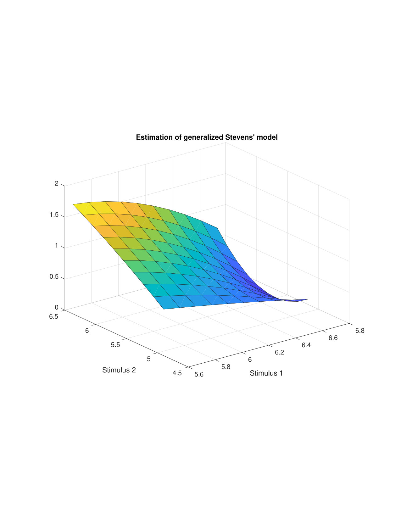 Figure 1
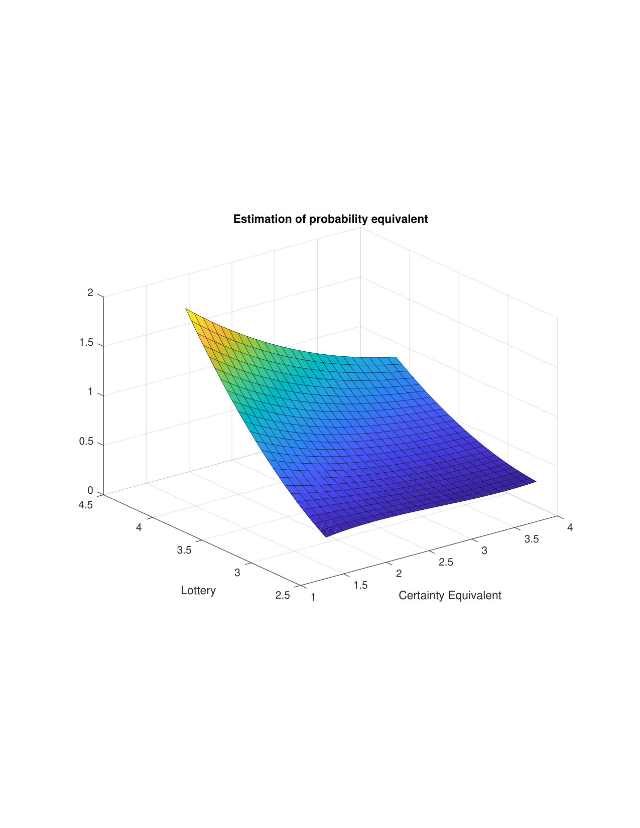 Figure 2
| Av. Prob. | |||
|---|---|---|---|
| Mean | 45.81 | 23.82 | 0.63 |
| St.Dev | 14.10 | 14.09 | 0.19 |
| Min | 13.00 | 4.00 | 0.26 |
| Max | 66.00 | 57.00 | 0.92 |
| Mean | 6.45 | 5.47 | 1.20 |
|---|---|---|---|
| St.Dev | 0.40 | 0.65 | 0.42 |
| Min | 5.51 | 4.82 | 0.64 |
| Max | 6.79 | 6.49 | 1.85 |
Peer Reviews
No public reviews on file for this paper yet. If you reviewed it on a platform where reviews are public (OpenReview, ICLR, NeurIPS, ICML), you can paste yours below so the community can read it here.
Videos
No videos yet. Explain this paper in a talk, walkthrough, or lecture? Add one.
Taxonomy
TopicsConsumer Market Behavior and Pricing · Decision-Making and Behavioral Economics · Economic theories and models
Nonparametric Estimation and Inference in Economic and Psychological
Experiments
Raffaello Seri, Samuele Centorrino, Michele Bernasconi
Università dell’Insubria, Stony Brook University, Università Ca’ Foscari
(Date: Last Version: March 17, 2024; First Version September 1, 2013)
Abstract.
The goal of this paper is to provide some tools for nonparametric estimation and inference in psychological and economic experiments. We consider an experimental framework in which each of subjects provides responses to a vector of stimuli. We propose to estimate the unknown function linking stimuli to responses through a nonparametric sieve estimator. We give conditions for consistency when either or or both diverge. The rate of convergence depends upon the error covariance structure, that is allowed to differ across subjects. With these results we derive the optimal divergence rate of the dimension of the sieve basis with both and . We provide guidance about the optimal balance between the number of subjects and questions in a laboratory experiment and argue that a large is often better than a large . We derive conditions for asymptotic normality of functionals of the estimator of and apply them to obtain the asymptotic distribution of the Wald test when the number of constraints under the null is finite and when it diverges along with other asymptotic parameters. Lastly, we investigate the previous properties when the conditional covariance matrix is replaced by an estimator.
This work was supported by a grant from MIUR (Ministero dell’Istruzione, dell’Università e della Ricerca). Authors would like to thank seminar participants at Stony Brook University, University of California Riverside and the 2016 UK Econometrics Study Group, especially Xavier D’Haultfoeuille, for useful comments and remarks.
1. Introduction
The aim of this paper is to provide a statistical theory useful for the nonparametric analysis of laboratory experiments in economics and psychology.
In the typical experiment we have in mind, there are subjects who are administered tasks. Task is characterized by , a -dimensional stimuli-vector that is the same for each subject , for . The response or choice of subject in task is denoted by . We suppose that the Data Generating Process (DGP) of the set of answers (, ) has a deterministic component represented by a nonparametric function of the stimuli, and a stochastic component arising from individual error terms. Hence, we have the system:
[TABLE]
The function can be interpreted as a deterministic theory that maps every value of the vector of stimuli to a space of real valued responses.
Equation (1.1) resembles a framework already discussed in experimental economics by Hey (2005), which involves a nonstandard econometric system, and encompasses several models arising in economics and psychologica experiments. To the best of our knowledge, however, a complete statistical analysis of this system has yet to be conducted. For instance, the vector can represent the prizes and the probabilities of a lottery presented in an economic experiment in which subjects are asked to give the certainty equivalent of the lottery. In this case, is the function used by subjects to evaluate the lotteries.111The present approach can be equally applied, though it may not be the most efficient, to situations in which is defined as , for two lotteries and presented to subjects in pairwise choice experiments, and is simply the choice (coded in some way) of subject . In psychophysical experiments, the vector can be thought to represent stimuli such as light, sound, weight, distance for which subjects are asked to assess in pairwise comparisons the relative magnitude. In this case, is the scale used by subjects to measure the stimuli. The fact that the explanatory variables are the same across individuals has a double justification: first of all, in many empirical studies the choice of the stimuli is so difficult that it is not possible to conduct it for each individual; second, when the regressors are the same across individuals the estimation problem is more difficult (in the sense that we have less information from the variation in the independent variables).
In statistics and econometrics, this model can be cast in the well-known and extensively studied framework of the nonparametric regression model (Li & Racine, 2007; Tsybakov, 2008). There are, however, several distinctive features of this model that make its analysis different and, in some respects, more challenging than the standard nonparametric regression. First, the realizations of the stimuli are not random observations from an underlying statistical distribution, but are chosen by the experimenter: the more complex the function one wishes to estimate, the richer the support of the data one needs to achieve consistency. Second, the statistical approach proposed in this work does not impose any specific restrictions on the structure of the error terms. In particular, it seems important that even if (1.1) holds true, the error terms for different individuals should be allowed to be differently distributed, provided . Among other things, this means that we allow different individuals to have different degrees of precision. This seems especially important in economics and psychology, when a researcher may have little to no knowledge about a theory that explains randomness in the responses. Also, individual variances may contain very persistent components, and, therefore, consistent estimation of an individual-specific response function may be unfeasible.222A similar statistical framework has been studied by Staniswalis & Lee (1998). While they also allow for the stimuli-vector to be time-varying, they suppose that the error term is a white noise.
Our goal in this paper is to study the nonparametric estimation of the function in (1.1) using the method of sieves (see Newey, 1997; de Jong, 2002; Chen, 2007; Belloni et al., 2015; Chen & Christensen, 2015, among others). The function of interest is approximated by a finite linear combination of some known basis functions (e.g., power series, regression splines, trigonometric polynomials), which effectively reduce the estimation problem to a finite number of parameters. The weights in the function approximation can be estimated through linear regression supposing that individuals and answers across individuals are independent. The number of approximating terms diverges to infinity with the sample size. We show that this estimator of the function is consistent, and we provide the convergence rate for this nonparametric estimator. We show that the convergence rate depends on the number of tasks (), the number of individuals (), and the number of basis functions used to approximate . Our convergence rate, however, also depends on the properties of the average covariance matrix across individuals for a given task . Heuristically, it thus explicitly takes into account the precision of the subjects in answering the questions and/or selecting specific choices.
We also provide asymptotic normality results for both linear and nonlinear functionals of the nonparametric estimator which are useful to obtain the asymptotic properties of the Wald test in this framework (Chen & Pouzo, 2015). We derive the properties of the latter both in the case where the number of constraints is finite (parametric restrictions), which gives the standard distribution under the null; and when the number of constraints diverges to infinity along with other asymptotic parameters (a normal distribution). Lastly, we investigate what happens when the average variance matrix appearing in the previous tests is replaced by an estimator. We believe inference is an essential part of our statistical theory, as it allows us to test specific behavioral assumptions.
Hey (2005) points out that underlying system (1.1) is the idea that the theory under investigation is deterministic, but that people apply the theory with noise. Such an approach, which is sometimes referred to as Thurstonian or Fechnerian, underlies for example the investigations conducted by Falmagne (1976), Orme & Hey (1994), Buschena & Zilberman (2000), and Blavatskyy (2007). Alternatively, other authors (including Camerer & Harless, 1994, Loomes & Sugden, 1995, Loomes et al., 2002, Myung et al., 2005) tend to interpret individual behavior in experiments (and possibly in the real world) as inherently stochastic, in the sense that while the theories remain deterministic, their predictions are not because of the imprecision of people to know and to use the same specification of the theory every time it is required.333For example, describing the philosophy behind the approach with reference to preference theories, Loomes (2005) argues that the approach “rather than supposing an individual to have a single true preference function to which white noise is added, … treats imprecision as if an individual’s preference consist of a set of such functions. Thus to say that a particular individual behaves according to a certain ‘core’ theory is to say that the individuals’ preferences can be represented by some functions, all of which are consistent with the theory; but that on any particular occasion, the individual act as if she picks one of those functions at random from the set, applies it to the decision at hand, then replaces that function before picking again at random in order to address the next decision” (p. 306). Antecedents of this approach can be found in Becker et al. (1963). It is also important to emphasize that this approach is still very different from the case in which the ‘core’ theory itself would be made inherently stochastic — as for example advocated by Luce (1997). The distinction between the two approaches, however, though quite interesting philosophically, is of practical relevance only when either of the following two circumstances applies. The first is when the dependence of the answers from the stimuli (according to function ) is parametric. In this case, the question of the two approaches turns into a fundamental question about whether the parameters to be estimated can be interpreted in deterministic terms or as random variables (as for example in the Bayesian approach pursued by Karabatsos, 2005, and Myung et al., 2005). The second applies to the specific restrictions on the errors terms which may be required by the statistical procedure used to analyze the experimental data (see for example Ballinger & Wilcox, 1997, for the discussions of several restrictions often imposed for the empirical analyses of data from decision theory experiments).
The present statistical approach is unaffected by both circumstances, so that it can be viewed to encompass both philosophies. First of all, a notable feature of the present approach is that the dependence of the answers from the stimuli is left nonparametric. Nonparametric dependence has the advantage that theoretical and/or behavioral properties of interest can be estimated and tested without the mediation of parametric restrictions, which (for the reasons just exposed) may not be unambiguously interpreted. Furthermore, nonparametric dependence is natural if one wishes to fit the experimental data without imposing any restrictions on behavior. Such ‘unrestricted’ model could be a useful benchmark against which to compare any structural model indicated by specific theories.444See Bernasconi et al. (2008, 2010b), for applications of such an approach in regards to experimental investigations of, respectively, psychophysical measurement theories and decisions theories.
As mentioned above, we also allow for the possibility that the precision of answers of the same individual varies across different questions. This is important because various previous studies have emphasized forms of heterogeneity occurring both at levels of individuals and of different experimental tasks (e.g., Ballinger & Wilcox, 1997; Buschena & Zilberman, 2000; Carbone & Hey, 2000; Blavatskyy, 2007; Butler & Loomes, 2007).
Finally, we should note that a long debated dispute in economic and psychological experiments is whether the analysis of the individual responses should be conducted for the aggregate of the individuals or individual by individual. The analysis presented here is primarily thought for the former case. In particular, depending on the degree of heterogeneity and precision of the experimental sample and of the theory one would like to test, large values of and/or of may have different impacts on the consistency of our estimator of the function and its derivatives.555An additional reason to prefer an aggregate analysis is that an experimenter may decide to assign different values of the stimuli to different subjects. Assuming that the assignment mechanism is random, the aggregate model would allow to approximate the function on a richer support. In this situation, the convergence rates presented in this paper constitute a worst-case scenario. If, however, one believes that the aggregate analysis cannot be carried forward because all individuals are characterized by different functions ,666In psychology, the risks of averaging across individuals when they are characterized by different functions has been stressed, e.g., in Skinner (1958, p. 99), Yost (1981, p. 212) and Bernasconi & Seri (2016). then our results apply verbatim, simply taking and letting the number of tasks to diverge. In this case, our analysis can be seen as an extension of the results in Newey (1997) and Belloni et al. (2015) to the case of deterministic regressors. Consistency is then guaranteed only under more stringent conditions on the variance of each individual error term.
The model in (1.1) can also be interpreted as a panel data specification in which the covariates vary only with . We do not pursue this interpretation further in this work, but we notice that Su & Jin (2012) have considered a panel data model with factor structure in the error term in which the function is allowed to vary across individuals, with . Notice, however, that time series data have a natural ordering that can be used in the asymptotic analysis, while our data do not possess such ordering. We show below that our convergence rates are amenable to some of their results, upon additional restrictions on the variance of the error term.
The present statistical approach is also suitable for various extensions which we indicate in the conclusions.
2. The Statistical Model
We recall that the data generating process is modeled as follows:
[TABLE]
where denotes the individual (or respondent) and denotes a specific task. The dependent variable and the vector of independent variables , where is taken to be a compact subset of .777Taking to be compact does not appear to be a strong restriction in this setting, as points are chosen by the experimenter possibly within a bounded interval. In the development of our theory, this assumption could be relaxed by substantially modifying our method of proof (see Chen & Christensen, 2015). In the following, we will suppose that the function belongs to a space that will not be specified explicitly: when in the discussion of the results we will suppose that has at least continuous derivatives, it is intended that will coincide with the Sobolev space .
This statistical models fits several experimental and quasi-experimental frameworks.
Example 1**.**
[Cumulative Prospect Theory] In the following, denotes the given lottery and the individual. Consider a gamble . Let be the certainty equivalent that the individual associates with the gamble, i.e. the certain monetary amount that makes her indifferent between the two. Cumulative Prospect Theory (CPT) starts from the following model:
[TABLE]
where is the utility function, is called the evaluation functional, which may or may not be equal to , and is the probability weighting function, that is taken to be strictly monotone increasing in . Supposing that , we get:
[TABLE]
Now, the experimental elicitation of the certainty equivalent has attracted critiques for its unreliability (see, e.g., Hershey & Schoemaker, 1985; Wakker & Deneffe, 1996; Harrison & Rutström, 2008; Luce, 1999, Section 1.2.2.1). Several authors have advocated instead to elicit the probability equivalent such that the individual is indifferent between and . The previous relation can be written as:
[TABLE]
We can write:
[TABLE]
where , for , and . Finally, supposing that the previous representation holds with some error , this implies:
[TABLE]
Example 2**.**
[Stevens’ Model] In ratio magnitude estimation, one of the most common form of psychophysical experiments, the aim is to evaluate the intensity of a set of stimuli with respect to a reference stimulus whose intensity is set to , thus justifying the alternative name of magnitude estimation with a standard (see, e.g., Luce & Krumhansl, 1988). In task of the experiment, an individual is proposed two stimuli, and , and asked to state the ratio of their intensities. One of the most well-known models in mathematical psychology is Stevens’ model, in which (see Stevens, 1975; Kornbrot, 2014; Bernasconi & Seri, 2016):
[TABLE]
It is generally, but not always, the case that and . Taking logarithms, we get . In order to estimate the model, we set and to get a regression model without intercept.
We now rewrite the model in equation (2.1) using matrix notations. We form the -vectors and . We suppose that has a distribution with mean [math] and variance , for every . We further define the -matrix obtained stacking the vectors . Finally,
[TABLE]
where the function is supposed to apply row-wise to the matrix . We make the following assumption about the vector of errors .
Assumption 1**.**
- (i)
The random vector is such that , for all , and , for all and .
- (ii)
Every element of is finite and the matrix is positive definite for all .
There are not noteworthy details in this assumption. We take the error terms to be uncorrelated across individuals and we impose some regularity conditions on the covariance matrix, which is otherwise left unspecified.
We now structure the statistical model for the whole data. We build the vectors and by stacking respectively the vectors and .
We finally have:
[TABLE]
where is a -vector of ones. is then a vector with mean [math] and variance , where denotes the direct sum of matrices. That is, .
Remark 3*.*
The fact that every individual is allowed to have a potentially different covariance matrix is a crucial characteristic in our setting. Consider a random function , and suppose that the decision model for individual is defined by the function , where is a drawing from a random variable , and denote , so that:
[TABLE]
Here the average is independent of the individual, but the error term is heteroskedastic (in the sense that it depends on the regressors) and heterogeneous (in the sense that it is different across individuals). In this setting, part of the correlation in the residuals is induced by the averaging across individuals, and conducting the analysis at the level of the single individual may improve inferences.
For estimation and inference, we take an approximation of using a linear combination of basis functions in . Thus, at , we take
[TABLE]
where is a vector of given basis functions and a vector of unknown coefficients, with , with . When , the dimension of the vector of stimuli, is larger than , then can be taken as a tensor product basis of total dimension . We also denote as
[TABLE]
the -matrix that stacks the approximating bases at every point . Then, we finally have:
[TABLE]
where
[TABLE]
The true value of the parameter , which we denote is taken to satisfy
[TABLE]
where the expectation is taken with respect to the distribution of for each individual . That is,
[TABLE]
The estimation of the model is performed by least squares, under the hypothesis that . Our sieve-based least-squares estimator is therefore given by:
[TABLE]
where denotes a matrix Kronecker product and we denote
[TABLE]
In some instances, we may omit the argument of the function, and simply use the notations and . Notice that the estimator (and the model itself) could be simply written as
[TABLE]
where is a vector of average individual responses for a given task . Our model could be then treated as any other nonparametric regression model with correlated errors. However, we believe this interpretation defies the entire purpose of our analysis. As a matter of fact, we would like emphasize the idea that the number of individuals performing the same task is essential when we cannot make standard regularity assumptions about the error term.
3. Consistency and Convergence Rates
We first define the norms:
[TABLE]
The norm is what is sometimes written as . We do not need to consider more general weighted Sobolev norms (see, e.g., Gallant & Nychka, 1987, for a definition), since the functions we consider have nonstochastic arguments.
Throughout the paper we will also need the following quantities. For every :
[TABLE]
where denotes the Frobenius norm. For every integer , we define:
[TABLE]
Denote and to be the largest eigenvalue and the trace, respectively, of the average covariance matrix of the errors .
The following assumption is needed to derive, together with the previous definitions, a uniform upper bound for the sieve estimator .
Assumption 2**.**
- (i)
As and any* , the matrix converges in Frobenius norm to a given positive definite matrix , whose smallest eigenvalue is bounded away from zero.*
- (ii)
For every , exists and for large enough .
The following assumption is needed to obtain consistency of the sieve estimator.
Assumption 3**.**
- (i)
We have:
[TABLE]
- (ii)
For , we require , as . For , we require , as .
Assumption 2 (i) restricts the asymptotic behavior of the matrix of design points . Notice that this assumption is not explicitly needed, e.g., in Newey (1997), de Jong (2002) and Belloni et al. (2015) as they deal with stochastic regressors and therefore this is guaranteed by an appeal to a Law of Large Numbers. In particular, Assumption 2 implies that the eigenvalues of converge to the eigenvalues of , for a fixed .
Newey (1997) and Belloni et al. (2015) derive rates of convergence in probability for towards the fixed matrix . Newey’s result implies that . However, we cannot use directly this result since our regressors are supposed to be deterministic. However, reasoning as in Reimer (1997), we can see that for any probability measure , so that it is possible to find a point-set such that .888Note that, from Belloni et al. (2015) (see their Section 6.1 and Theorem 4.6), one can infer that from which one gets the weaker bound . Better convergence rates can be obtained in special cases (see the discussion after Theorem 5).
Remark 4*.*
Define the empirical probability . A particular case is the one in which the points are chosen in such a way that their empirical probability converges to an asymptotic design measure on . In this scenario, we can obtain explicitly as , where is the expectation taken with respect to the probability . This situation is similar to the one in Cox (1988). In our case, it is unnecessary to specify the asymptotic design measure but, when available, it can be used to derive an explicit expression for .
Assumptions 2 (ii) and 3 (ii) are used to bound the approximation error and to define a uniform upper bound on the derivative of the vector of basis functions, as measured through the Sobolev norm, both of which are standard assumptions in the sieve literature. When the function is taken to be times continuously differentiable, we can take (see Newey, 1997; Huang, 2003; Chen, 2007; Belloni et al., 2015).
Assumption 3 (i) restricts the behavior of the largest eigenvalue and the trace of the average covariance matrix of the errors . Depending on the structure of the covariance matrix, these quantities may or may not be uniformly bounded away from infinity.
Under the previous assumptions, it is possible to derive an upper bound for the convergence rate of to .
Theorem 5**.**
Under Assumptions 1 and 2, the following bound can be established:
[TABLE]
Under Assumption 3, the bound converges to 0 and the sieve estimator is a consistent estimator of in the norm.
Assumption 3 ensures that the upper bound of Theorem 5 is as . Notice that, if is taken to be finite and and are uniformly bounded away from infinity, the upper bound of the variance in Theorem 5 is the same as in Newey (1997).
Remarks on and
The terms and that enter the formulas have a behavior that can be clarified in some cases of interest.
A first case arises when the answers for a given individual are supposed to be uncorrelated to each other (even if heteroskedastic), so that . Define . In this case, , and , so that the bound in Theorem 5 yields:
[TABLE]
If is bounded, the bound does not make any difference between and . Assumption 2 (i) requires that , so that also is sufficient to ensure consistency, provided that . In this case our estimator reduces to the one in Newey (1997). Despite our assumptions are not comparable with the ones in Newey (1997), as we consider the case of deterministic regressors, ours are generally weaker as we require uncorrelatedness and boundedness of the variances of the errors whereas he requires independence and identical distribution. Lack of dependence between tasks and boundedness of the maximum variance allow one to estimate consistently individual response functions. The hypothesis that the average covariance matrix of the errors is diagonal could be in principle tested. However, we have not been able to find in the literature a test valid under our conditions, i.e. for possibly non identically distributed error vectors of increasing dimension. We leave the development of such a test to future work.
A second case of interest arises when the errors for every individual have a factor structure, i.e. every error term can be written as where , , for , and , for all . This means that the matrix can be written as
[TABLE]
According to Lemma 2.1 in Magnus (1982), , and we obtain . The bound in Theorem 5 implies that
[TABLE]
If the number of tasks is held fixed and the number of respondents is allowed to diverge to infinity, one could strengthen Assumption 2 (i) to allow for the design matrix to be nonsingular for any finite value of and such that . However, the finiteness of implies that the bias component does not disappear asymptotically and thus the estimator is not consistent. Similarly, if the number of individuals is held fixed and , while the bias vanishes, the variance does not disappear asymptotically, and again the estimator is not consistent. In our framework, however, letting both yields a consistent estimator of . Parametric rates of convergence can be achieved for when , i.e. when both and diverge sufficiently fast. Nonparametric rates for specific choices of the sieve basis are discussed in the Appendix.
Example 6**.**
[Stevens’ Model; Example 2 continued] We suppose that Stevens’ model is the true model that generates the data. We estimate the model as
[TABLE]
This is a case of parametric estimation. Assumptions 1 and 2 are supposed to be true. Moreover, is finite and is [math]. The rate of convergence is therefore .
Example 7**.**
[Cumulative Prospect Theory; Example 1 continued] Consider the model of Example 1. We consider the estimation of a model of the form:
[TABLE]
using a tensor product of Legendre polynomials:
[TABLE]
If the parameters are chosen as in Section 2, we denote the function as . Let us denote as a polynomial of order and let be the one with parameters chosen as in Section 2. Then, . Using Theorem 2 in Calvi & Levenberg (2008) we get . From Bos & Levenberg (2018) (see also Trefethen (2017)), supposing that is analytic, for . At last, when :
[TABLE]
A similar bound clearly applies when . Therefore, using the fact that :
[TABLE]
If the errors have a factor structure, then:
[TABLE]
Example 8**.**
[Stevens’ Model; Example 2 continued] In this case too, as in Example 6, we suppose that Stevens’ model holds true but we consider a more general nonparametric model in log-log form (see Bernasconi et al., 2008 for a justification):
[TABLE]
where is an unknown function. We approximate the function using a polynomial of order in the two variables and :
[TABLE]
This polynomial regression has parameters. Assumptions 1 and 2 are verified, provided is chosen correctly. Provided , we have and Assumption 3 (ii) is automatically true. The rate of convergence is:
[TABLE]
If the errors have a factor structure, the bound becomes and Assumption 3 (i) requires to ensure uniform convergence of mixed partial derivatives up to order , which, for finite , is a standard condition on the sample size.
Regression Models with Individual-Specific Characteristics
To conclude this section, we briefly discuss the possibility of augmenting the model to include subject characteristics, which we denote by . In most experiments, these characteristics are inherently discrete (e.g., age, treatment group, gender, etc.). Assume for simplicity that the th element of the vector can take values with strictly positive probability. Therefore, every element of can be decomposed into dummy variables, each one taking value if , and [math] otherwise, for . Without loss of generality, we can thus define , where is a positive integer, and can also include arbitrary interactions between the observed individual characteristics. For such a binary random vector, we impose that the joint function is such that , whenever all the elements of are equal to [math]. Hence, we can write any joint function , which follows from the fact that its value changes in only when is equal to , for . This finally implies the following statistical model
[TABLE]
where the unknown functional coefficients depend on This nonparametric regression can be cast as a varying coefficient model (see, e.g., Hastie & Tibshirani, 1993; Fan & Zhang, 1999; Fan & Huang, 2005). In this flexible semiparametric framework, we can include an arbitrary number of individual specific covariates without incurring the curse of dimensionality. Letting , the vector satisfies the following system of moment restrictions
[TABLE]
where the last equality follows from the fact that the vector should be determined independently of individual’s characteristics, and therefore all the moments of the distribution of are independent of . For identification, we only require the additional condition that the matrix is full rank. A nonparametric sieve estimator of the functional coefficients can be obtained by simply replacing the function with some finite dimensional approximation on a space of basis functions, and the unknown population moments of with their sample counterpart. Estimation of this model is equivalent to splitting the sample in subsamples, and estimate the unknown regression functions for each one of these subsamples. However, joint estimation of the vector of coefficients is naturally more efficient, because it uses the entire sample size. Hence, the resulting sieve estimators inherit the same properties as above (see Fan & Zhang, 2008).
4. Asymptotic Normality and Wald Tests
In the following we investigate the asymptotic normality of functionals of our nonparametric estimator. These are useful to study the properties of classical statistical tests. We focus here on the properties of the Wald test and we provide its bias and the rates of convergence to its asymptotic distribution: we choose this strategy to be able to evaluate accurately the interplay between the different asymptotic parameters appearing below. We do not discuss whether it is possible to estimate these functionals at -rate. Arguably, one could extend the results in Newey (1997) to our setting to provide such results.
In the following, we consider estimation of a functional of the function . As in Andrews (1991), we write this functional as , where denotes the number of restrictions. Note that is allowed to depend on and . We provide conditions for asymptotic normality of the quantity
[TABLE]
where and . First of all we consider the case in which is linear, then we will move to the nonlinear case.
4.1. Linear Case
We consider both the case in which is fixed and the case in which diverges with and . The case when is allowed to increase with and will be particularly useful to derive the asymptotic properties of Wald tests. We suppose that when applied to the functional yields:
[TABLE]
where can take different values according to the linear functional . A full list of examples is in Andrews (1991, p. 310), but some very simple instances are the following ones:
- (1)
Pointwise evaluation functional: , and ; 2. (2)
Pointwise partial derivatives: and ; 3. (3)
Weighted average derivatives: and for a given probability distribution on .
All of these examples can also be considered in vector form, as in Andrews (1991, p. 310).
The variance of the linear functional applied to an estimated function, namely , is given by:
[TABLE]
where . Provided is symmetric positive definite, let be the symmetric positive definite square root of the inverse of .
We decompose in two parts: an error term
[TABLE]
and a bias term
[TABLE]
We provide conditions under which the first term converges in distribution to a dimensional standard normal vector and the second term tends to a null vector. The vector enters in the formula of the Wald test for the hypothesis :
[TABLE]
In the following we will consider a standardized version of the statistic, namely . This is particularly useful when the number of constraints is allowed to increase with and , as we show below.
Example 9**.**
[Pointwise Constraints] A first case of interest arises when we want to constrain the function at a point. Then is a pointwise evaluation functional. Consider the situation in which and we want to test whether the function can be constrained in a point, say , to take value where . Consider the following regression model using a power series of order :
[TABLE]
The test concerns the null hypothesis . For a fixed , we use the Wald test statistic above with
[TABLE]
Example 10**.**
[Cumulative Prospect Theory; Example 1 continued] As customary in this literature (see, e.g., Luce, 1999, Section 3.1), we assume that . Moreover, one can suppose that the utility function can adequately be described by power functions with exponent (see, e.g., Luce, 1999, Section 3.3). Therefore:
[TABLE]
and the model becomes a semiparametric one with
[TABLE]
We would like to provide a test for the parametric restriction in equation (4.1), for any . Under the null hypothesis, we have that:
[TABLE]
This null hypothesis cannot be tested directly, as such a test would require the estimation of the transformation function . Therefore, we proceed as follows. Under the null, we take the derivatives of the regression function wrt and respectively. We obtain:
[TABLE]
Therefore, the sum of these two derivative must be equal to [math] almost everywhere. Omitting the arguments of the function for simplicity, our null hypothesis can be written as
[TABLE]
This is a linear functional of the nonparametric estimator. To avoid the clumsy notation, let us write and . Let be the row vector of the first Legendre polynomials evaluated in . We approximate through the tensor product function where and can be different. Taking the derivative with respect to we get , where is a strictly upper triangular -matrix called operational matrix of differentiation for Legendre polynomials. Formulas for this matrix have been derived in Sparis & Mouroutsos (1986); Sparis (1987), using a detour through power series, and Bolek (1993), using a direct approach based on formulas for the derivatives of Legendre polynomials (see also Phillips, 1988). Therefore:
[TABLE]
From this
[TABLE]
and, at last:
[TABLE]
Matrices of this kind are sometimes called Kronecker sums (see Canuto et al. (2014); Benzi & Simoncini (2015)) and indicated as (the symbol is sometimes also used for the direct sum of matrices, as in our Section 2). Exactly rows and columns of the -matrix are not linearly independent of the others, thus giving a total of linearly independent restrictions.
Example 11**.**
[Stevens’ Model; Example 2 continued] In order to test Stevens’ model, we consider the model of Example 8. We want to test the statistical hypothesis . The test is then obtained imposing the constraints and . We use the test statistic above with:
[TABLE]
In this case and we would like to find conditions such that can increase with and .
We make the following assumptions.
Assumption 4**.**
- (i)
The function .
- (ii)
* is a uniformly bounded sequence of linear functionals. That is, is linear and for some constant (that can depend on , or ) and integer such that , one has for all and .*
- •
When applied to , it yields .
Assumption 5**.**
- (i)
For fixed and , .
- (ii)
The error term is such that
[TABLE]
for some .
Assumption 6**.**
For fixed and , .
Theorem 12**.**
- (i)
Let be the identity matrix of dimension . Then
[TABLE]
- (ii)
The following bound on the bias can be established:
[TABLE]
where is the value of the index for which Assumption 4 (ii) holds.
- (iii)
The standardized Wald test whose test statistic is given by can be decomposed as:
[TABLE]
where the distribution of is such that
[TABLE]
(irrespectively of the fact that is fixed or goes to infinity), or
[TABLE]
where is a standard normal random variable.
Remark 13*.*
The bounds in part (iii) of this theorem use the theoretical results in Bentkus (2004), who provides a Berry-Esséen bound for independent non-identically distributed random variables. For i.i.d. vectors , the first part of these bounds would not depend on the number of constraints (see Bentkus, 2003).
Example 14**.**
[Pointwise Constraints; Example 9 continued] The linear functional is and , so that . The variance is given by
[TABLE]
Assumptions 1, 2, 4 (i) and 6 hold if is well-chosen. Letting , and supposing that with and that , Assumption 3 holds provided . Assumption 4 (ii) holds since and we can use the upper bound to state that and . Assumption 5 (i) can be supposed to be true. Then, Assumption 5 (ii) leads to a constraint on the relative rate of increase of and : if, taking , is bounded from above and from below uniformly in and , we need . The test statistic is:
[TABLE]
The rate of decrease of the bias is given by:
[TABLE]
where we have used . This means that we need to get consistency of the sieve estimator and convergence to 0 of the bias of the Wald test statistic, while asymptotic normality requires .
Example 15**.**
[Cumulative Prospect Theory; Example 1 continued] The matrix is the sum of the partial derivatives of with respect to and , respectively. The variance can thus be written as in Example 14. Assumptions 1, 2, 3, 4 (i) and 6 hold whenever is chosen appropriately. We assume that , so that . In this example, we further consider the space , and denote as its Sobolev norm. Notice that these operators are bounded in , as a function in with norm equal to must admit a derivative with finite norm. Therefore, we obtain
[TABLE]
and Assumption 4 (ii) holds with . The number of restrictions and the test statistic can be written as
[TABLE]
If is analytic, using Example 7, the order of the bias is
[TABLE]
Now, suppose that and that () is bounded uniformly from above (below). Therefore, can be approximated by if and by if, in addition, .
Example 16**.**
[Stevens’ Model; Example 2 continued] The variance can be written as above. Assumptions 1, 2, 3, 4 (i) and 6 hold whenever is chosen appropriately. Now, where the ’s are the coefficients in the power series expansion of the function . Using Young’s inequality, we obtain
[TABLE]
Therefore, Assumption 4 (ii) holds with . Under the null hypothesis of the test, the bias is exactly [math]. Assumption 5 (ii) leads to a constraint on the relative rate of increase of and : if, for some , is bounded from above and from below uniformly in and (thus respecting Assumption 5 (i)), we need . The test statistic is:
[TABLE]
This can be approximated by if and by if, in addition, .
4.2. Nonlinear Case
Now we pass to consider asymptotic normality of nonlinear functionals, also denoted as . Our treatment extends the one in Theorem 2 in Newey (1997) to the multivariate case. We suppose that possesses a directional derivative enjoying the properties stated in Assumption 4 (ii). When the second argument of is the true function , we simply write . In case of nonlinear functionals, we replace Assumption 4 (ii) with the following.
Assumption 7**.**
* is a nonlinear functional for which a function exists such that:*
- (i)
* is linear in ; when applied to , it yields .*
- (ii)
For some and for all , such that and , the inequalities:
[TABLE]
hold.
- (iii)
* for all and .*
The variance and its square root entering the statement of the theorem have exactly the same definition as above, with defined as in Assumption 7 (i). In this case the decomposition of into an error and a bias term has a parallel in the decomposition into a linear part and a remainder part (that is not strictly speaking a bias since it is random and depends upon ). The linear part provides the asymptotic distribution and the remainder has to be bounded adequately.
Theorem 17**.**
Let Assumptions 1-3, 4 (i), 5-7 hold.
- (i)
The following asymptotic distribution holds:
[TABLE]
- (ii)
The following bound on the remainder can be established:
[TABLE]
where is the value of the index for which Assumption 7 (iii) holds.
- (iii)
The standardized Wald test whose test statistic is given by can be decomposed as:
[TABLE]
where respects the Berry-Esséen bounds of Theorem 12 (iii).
4.3. Estimation of the Variance Matrix
In this section we provide some results about the effect of replacing with an estimator . Wald-type tests require the replacement to occur in the test statistics but have standard asymptotic distributions: in this case, we provide a bound on the absolute error of the replacement in .
Theorem 18**.**
Define the residuals
[TABLE]
and the estimated average covariance matrix . Consider the setting of Theorem 12. Let be the quantity obtained replacing with . Let Assumptions 1-4 or Assumptions 1-3, 4(i), 5-7 hold. If
[TABLE]
then
[TABLE]
Remark 19*.*
It is clearly possible to regularize the matrix before replacing in . However, as our asymptotic normality results generally require and under this condition it is expected that has full rank, the regularization should have a limited impact on the performance of the tests.
Example 20**.**
[Pointwise Constraints; Example 9 continued] Suppose that is bounded from below and from above uniformly in and . Since , and we have:
[TABLE]
Since the first term on the right hand side is , whenever the replacement has no asymptotic effect on the asymptotic distribution of the Wald test. Note that is automatically respected whenever the condition for asymptotic normality in Example 14, i.e. , is satisfied.
Example 21**.**
[Cumulative Prospect Theory; Example 1 continued] If () is bounded uniformly from above (below), the condition becomes:
[TABLE]
Here is the condition number of the Gram matrix .
Our derivations contained in the Appendix imply that
[TABLE]
Example 22**.**
[Stevens’ Model; Example 2 continued] Suppose that is bounded from below uniformly in and and is bounded from above. In this case is the matrix described in Example 11 and so that and . If :
[TABLE]
In some cases, it can be of interest to estimate the conditional variance as a function of observable characteristics of the stimuli and/or the individuals (see, e.g., Butler & Loomes, 2007). We will investigate this alternative procedure rather informally. Suppose that the following model holds:
[TABLE]
where the vector shares some of the features of and it may also coincides with it. The latter implies, among other things, that the variance is the same across individuals but different across questions.
Example 23**.**
[Remark 3 continued] In this case:
[TABLE]
We can write:
[TABLE]
where . Unfortunately, the error is not available but can be replaced by the residual . Therefore, we can use the equation
[TABLE]
If the objective is to estimate the entire structure of the matrix as a function , we are left with the problem of estimating covariances. A potential solution is to suppose that errors are equicorrelated, in which case the correlations can be estimated from the standardized residuals. We do not pursue this topic here.
5. Applications
We now apply our estimation procedure to two simple examples introduced above in Economics and Psychology. In both examples, we estimate the unknown function nonparametrically, and then we use the Wald statistics to test meaningful restrictions either on the function itself or on its derivatives.
The function is approximated using tensor products of Legendre polynomials, which make the estimation and testing procedures straightforward and intuitive. We denote as , the Legendre polynomial of order , with . The order of the polynomial is chosen by cross-validation (Hansen, 2014).
5.1. Cumulative Prospect Theory
We now use the results in Examples 1, 7, 10, 15 and 21 to analyze the data of an economic experiment. We employ a classical experimental design to elicit the preference of an individual in choice under uncertainty. The elicitation procedure is known as the probability equivalence method and is dual to the certainty equivalence method. It works as follows. In a sequence of pairwise comparisons for , an individual is asked to state the probability that would make the individual indifferent between receiving the sure amount of money or a lottery giving the monetary prize with probability and [math] otherwise.
Thus, in the probability equivalence method and are the stimuli and the response, whereas in the certainty equivalence method and are the stimuli and the response. We also remark that, though both methods are in principle capable to elicit the preferences of the individual, since their early applications it is known that both methods can lead to various types of inconsistencies. For this reasons, various proposals of revising the basic elicitation procedures have been made in the literature in attempt to control for the inconsistencies (references and discussion in, e.g., Hershey & Schoemaker, 1985; Wakker & Deneffe, 1996; Abdellaoui, 2000).
Both elicitation procedures are nevertheless very simple and are useful for the purpose of illustrating our nonparametric method of estimation and inference. We in particular conducted the probability equivalence experiment with 98 participants (). Each of them gave the responses ’s to 100 questions (). The 100 questions employed monetary prizes distributed uniformly between a minimum of 15 Euro and a maximum of 66 Euro, with the sure amount varying between a minimum of 4 Euro and a maximum of 57 Euro. The experiment was run individually and was computerized: questions were presented sequentially to each individual on a computer screen, with the order of the questions randomized independently for each participant. Each participant had the opportunity to reconsider the decision to each individual questions several times before confirming it; but once confirmed, the computer moved the participant to another question and previous choices couldn’t be any longer revised or accessed. At the end of each individual experiment one question was randomly selected for each participant and each participant was paid according to the choice he or she made in the selected question. In particular, participants were incentivized to give correct answers by the use of the standard Becker et al. (1964) payment method.
A summary of the distribution of , , and the sample mean of across individuals is reported in the Table 1.
With these data, we first estimate the following fully nonparametric regression model:
[TABLE]
using a tensor product of polynomials of order in and polynomials of order in . Figure 5.1 depicts the nonparametric estimator of the regression function .
To implement the testing procedure, we slightly undersmooth compared to the estimation above, and take a cubic polynomial in and a quartic polynomial in (see Theorem 12). Therefore, we have a total of restrictions, but only 16 of them are linearly independent. As and , these restrictions are:
[TABLE]
and:
[TABLE]
The value of the test statistic is , which leads to a rejection of the null hypothesis, with a value strictly lower than . This implies that the usual power specification of the utility function may not be justified in our setting, and such an assumption could lead to an inconsistent estimation of the probability weighting function.
5.2. Stevens’ Model
Now we consider an experimental application related to the model in Examples 2, 6, 8, 11, 16 and 22. The only difference with respect to the examples is that we use Legendre polynomials, but this has no impact on the conditions. In the experiment, individuals were asked to give their estimates of ratios of distances of pairs of Italian cities from a reference city. Participants were undergraduate students in economics from the University of Insubria in Italy. We presented to the subjects 10 pairs of Italian cities and we asked them to estimate the ratio of their distances with respect to Milan: the pairs were given by all the possible combinations out of the five cities Turin, Venice, Rome, Naples and Palermo. The range of the stimuli goes from 124 to 885 km and the range of the real distance ratios from 2 to 7.137. We asked participants, first, to state for each comparison which of the two items they thought was larger, and then to quantify the relative dominance of the two items, i.e. how many times the city that they considered more distant from Milan was, according to them, actually more distant from Milan than the city they considered less distant. All the experiments were performed in a random order. The data were already analyzed, with different aims and techniques, in Bernasconi et al. (2010a, 2011, 2014).
A summary of the magnitude of the stimuli and of the ratio reported by the individual is given in Table 2.
A nonparametric series estimator of the function of Example 8 is reported in Figure 5.2. We take quadratic polynomials in both and .
We test Stevens’ model (see Examples 2 and 6), in which is a linear function of the difference of the log between the two stimuli. That is, our null hypothesis is:
[TABLE]
for some real . The test for this hypothesis has been considered in Examples 11, 16 and 22. Under the null hypothesis, the intercept of the model is equal to zero; the two slopes sum up to zero; and all other higher-order coefficients are equal to zero. We therefore tests restrictions on the vector of estimated parameters. We remark that the number of individuals is much larger than the number of questions , thus providing some support for the conditions in Example 16.
In this case, we do not undersmooth to implement our testing procedure, since the quadratic tensor product basis already exhausts the degrees of freedom in our model. The value of the test statistic is , which leads to a rejection of the null hypothesis, with a value strictly lower than .
6. Conclusions
We present in this paper a set of statistical tools useful for the analysis of some experimental data when the researcher aims at estimating and testing the average individual response function nonparametrically. In lack of a theory of errors in either economic or psychophysical experiments, we allow our regression errors to be correlated within individual tasks, and to feature heteroskedasticity between different individuals. In particular, and differently from a large body of literature on nonparametric regressions, we do not assume that variance of the error term is uniformly bounded away from infinity. This approach makes the tools we suggest robust to several structures of the error covariance matrix, for which theory often provides scarce or contradictory information. We finally point out that our results can be considered a worst-case scenario. That is, we only consider the case when the same tasks are submitted to all individuals. We conjecture that better asymptotic properties could be obtained if one allows for different individuals to perform different tasks. We defer the analysis of such a case to further research.
7. Appendix
7.1. Rates of convergence for specific choices of the sieve basis in Theorem
Parametric estimation
We briefly consider the case of parametric estimation. In this case, we have , and and fixed. It can be interesting to remark that in order to have consistency in this context Assumption 3 (ii) is not even necessary. The convergence rate is:
[TABLE]
It is further possible to show that this is near to the correct rate of convergence. Indeed, we have:
[TABLE]
and, using the assumptions stated above, the only difference is the replacement of with .
Fully nonparametric models - Power series
Let us look at what happens for power series. In this case, the order of the polynomial is linked to through the relation , where is the number of regressors and the asymptotic equivalence holds for : this means that it would be possible to obtain bounds in from bounds in . In this case (see Newey 1997, p. 157), , while the two best known results for are for , and for , where is the number of continuous derivatives of .
When , the bound becomes:
[TABLE]
Suppose first that . Then the bound is , and in order for this to converge to [math], we need at least and . The best convergence rate can be obtained when . In this case the bound is:
[TABLE]
Suppose now that . Then the bound becomes , and we need at least and to get consistency. The best convergence rate is obtained when , yielding:
[TABLE]
As concerns for analytic functions, we consider only the case and (see Example 7 for the case ): it is well known that , where can be explicitly characterized. Moreover, supposing that , the rate of convergence for the optimal is:
[TABLE]
where the first bound holds for and the second for . These are close to the rates of convergence for the parametric case.
We notice that in the case of power series regression, the quantity can be bounded in a more efficient way than the one after Assumption 3: this also provides some hints about how an experiment can be designed in order to efficiently approximate . Suppose that we can take the compact space as the unit hypercube and the asymptotic design measure (see Remark 4) as the uniform probability measure on . Then we can use the results of Klinger & Tichy (1997) on the polynomial discrepancy of sequences. In order to do so, we write as the -th element of and as the -th element of . Therefore, every element can be written as for a certain multi-index of non-negative integers. Using the definition of the Frobenius norm, we have:
[TABLE]
where and are the unanchored and the star discrepancies of the sample of points. Therefore:
[TABLE]
Remark that if is a low-discrepancy sequence, the discrepancy can be made to converge to [math] as fast as , so that . On the other hand, random sampling provides a rate of , if one considers the Frobenius norm (see Newey 1997, pp. 161-162), or , where denotes the spectral norm (see, Belloni et al. 2015, Theorem 4.6). Our bound thus improves over existing results, at least in this particular case.
Fully nonparametric models - Regression splines
In the case of regression splines (see Newey 1997, p. 160), , while the only two known results for are for , and for , where is the number of continuous derivatives of .
We focus on the case . Suppose first that . In this case, the bound becomes:
[TABLE]
In order for this to converge to [math], we need at least and . The best convergence rate can be obtained when . In this case the bound is:
[TABLE]
Suppose now that . The bound becomes:
[TABLE]
In this case we need and . The best convergence rate can be obtained when . In this case, the bound is:
[TABLE]
7.2. Proof of Example 21
Example 24**.**
In order to get an upper bound on this number, we first provide an upper bound on the largest eigenvalue . Recall from Example 10that . Thus
[TABLE]
Let () be the vector of Legendre polynomials (power series) evaluated at , that can be written as . The tensor product of the Legendre polynomials can be thus written as
[TABLE]
and
[TABLE]
Taking the derivative with respect to we get , with
[TABLE]
a super-diagonal matrix. We thus have
[TABLE]
where, to avoid notational cluttering, we let and be the identity matrices of dimension and , respectively. From this
[TABLE]
and:
[TABLE]
This means that the matrix defined in Example 10 is given by (see Section 3 in Sparis & Mouroutsos (1986)). The matrix has rank , so that we have:
[TABLE]
We note that, by Theorem 2 in Zielke (1988):
[TABLE]
Now we characterize the matrices . As we aim at using the results of Farouki (1991, 2000), we introduce the matrices of the following transformations, namely the basis-transformation matrix from Bernstein to Legendre polynomials and the equivalent matrix from power to Bernstein polynomials . Clearly, . Therefore:
[TABLE]
where (Farouki (2000)) and (Farouki (1991)). Then:
[TABLE]
Now, is a strictly upper triangular -matrix. The first column and the last row of are filled with zeros and can be removed to get an upper triangular -matrix , where the non-zero singular values of these two matrices are the same. With standard inequalities, it is hard to get a lower bound on this eigenvalue that is not negative. However, through some numerical experiments, we have obtained
[TABLE]
which finally implies our result.
7.3. Proof of Theorem 5
We start remarking that under Assumption 2:
[TABLE]
and wlog the matrix can be taken to be the identity matrix of dimension , . Therefore, converges to . We define the indicator function . Clearly, . Moreover, under Assumption 1, we write as , where , and , where .
The following lemma is useful in the proof of the main theorem.
Lemma 25**.**
[TABLE]
Proof.
We have:
[TABLE]
from which:
[TABLE]
For the first term in the sum, we get two different bounds. First, we proceed as follows:
[TABLE]
For the first version of the bound, we use the following majorization:
[TABLE]
This implies, from Markov’s inequality, that:
[TABLE]
For the second version of the bound, we write:
[TABLE]
where the last inequality comes from idempotence of . From Markov’s inequality, we finally get:
[TABLE]
Similarly, using the idempotence of , we have that
[TABLE]
The result of the lemma follows. ∎
The bound stated in the theorem comes from the majorization:
[TABLE]
The theorem follows from Lemma 25 and Assumption 3.
7.4. Asymptotic Normality and Wald Tests
Proof of Theorem 12. (i) First of all we show that is well defined. We have , and:
[TABLE]
from Assumptions 5 (i) and 6. Therefore is well defined. From Assumption 4 (ii), we have and . Therefore:
[TABLE]
We use the Cramér-Wold device (with such that ) applied to :
[TABLE]
where . We verify Lyapunov condition:
[TABLE]
where the first and second steps come from properties of norms, the third from the Courant-Fisher variational property of eigenvalues, and the fourth from idempotence. An upper bound on this function can be obtained as follows:
[TABLE]
where the last step comes from Loéve’s inequality (we recall that this is the inequality where if and if ).
(ii) Take . By Assumption 4, we have:
[TABLE]
and:
[TABLE]
Let be a vector such that . Using the Courant-Fisher variational property of eigenvalues, we obtain the inequality:
[TABLE]
and from this, using :
[TABLE]
We have:
[TABLE]
where the first inequality is Cauchy-Schwarz’ and the second inequality uses (7.4) and the idempotence of . Similarly,
[TABLE]
where the first inequality is Cauchy-Schwarz’, the second inequality, i.e. , comes from the Courant-Fisher variational property of eigenvalues, and the last inequality from (7.1).
(iii) We can write:
[TABLE]
where
[TABLE]
First of all, we want to find conditions under which approaches a Gaussian random vector when and (and sometimes ) diverge to infinity. We take
[TABLE]
where is the ball of radius in . For a standard Gaussian vector we have
[TABLE]
To bound this quantity, we express as in (7.2) and we use the Berry-Esséen bound of Theorem 1.1 in Bentkus (2004):
[TABLE]
Notice that, since , the normalization condition of the theorem is respected. The right-hand side of the previous equation can be majorized using ((7.3)) with . We get
[TABLE]
Then, respectively from part (ii) and part (i) of the present theorem:
[TABLE]
Summing up:
[TABLE]
The approximation of through a standard normal random variable proceeds using the classical Berry-Esséen bound for sums of independent identically distributed random variables.
Proof of Theorem 17. First of all, we decompose the quantity as follows:
[TABLE]
We will show in the following that the dominating term is while all the others converge to [math]. Therefore, we compute the variance of the term, that we call
[TABLE]
where . Provided is symmetric positive definite, let be the symmetric positive definite square root of the inverse of . The positive definiteness of is checked as in the proof of Theorem 12 under Assumptions 5 (i) and 6. At last, we can decompose the normalized vector in a linear part (yielding the asymptotic distributional result):
[TABLE]
and a nonlinear part (that does not contribute to the asymptotic distribution):
[TABLE]
As concerns the linear part, asymptotic normality of is verified as in Theorem 12.
Now we provide an upper bound for the nonlinear part. We start remarking that:
[TABLE]
The first term is:
[TABLE]
The second term can be upper bounded as in Theorem 12, replacing Assumption 4 with Assumption 7 (i) and (iii).
7.5. Estimation of the Variance Matrix
Proof of Theorem 18. First of all, we derive some general results about that will be needed for the Wald tests. We will need to consider the quadratic form , that can be written as follows:
[TABLE]
Defining and , we write as:
[TABLE]
Therefore:
[TABLE]
and:
[TABLE]
We need and we can majorize it as:
[TABLE]
Here
[TABLE]
Now we majorize the other term. In the general case, we have . Now:
[TABLE]
where we have used the Cauchy-Schwarz’ inequality to bound the terms with . Therefore:
[TABLE]
This is the bound we will use in the following proofs.
(i) We are led to study . We want to obtain:
[TABLE]
Now:
[TABLE]
where and is a perturbation of . Here .
In Mathias (1997, Th. 2), the following bound for matrices can be found:
[TABLE]
where and . Remark that the case leads directly to the majorization and that . Alternatively, we can write it as:
[TABLE]
In our case we have:
[TABLE]
where:
[TABLE]
and:
[TABLE]
that is:
[TABLE]
The term is bounded under Assumption 2. If :
[TABLE]
where we have used the previously derived bound on and the Weyl inequality for the smallest eigenvalue. Now:
[TABLE]
Therefore, provided :
[TABLE]
The result of the theorem follows.
The reference list from the paper itself. Each links out to its DOI / PubMed record.
- 1(1)
- 2Abdellaoui (2000) Abdellaoui, M. (2000), ‘Parameter-free elicitation of utility and probability weighting functions’, Management Science 46 (11), 1497–1512.
- 3Andrews (1991) Andrews, D. W. (1991), ‘Asymptotic normality of series estimators for nonparametric and semiparametric regression models’, Econometrica 59 (2), 307 – 345.
- 4Ballinger & Wilcox (1997) Ballinger, T. P. & Wilcox, N. T. (1997), ‘Decisions, Error and Heterogeneity’, The Economic Journal 107 (443), 1090–1105.
- 5Becker et al. (1963) Becker, G. M., De Groot, M. H. & Marschak, J. (1963), ‘Stochastic models of choice behavior’, Behavioral Science 8 (1), 41–55.
- 6Becker et al. (1964) Becker, G. M., De Groot, M. H. & Marschak, J. (1964), ‘Measuring utility by a single-response sequential method’, Systems Research and Behavioral Science 9 (3), 226–232.
- 7Belloni et al. (2015) Belloni, A., Chernozhukov, V., Chetverikov, D. & Kato, K. (2015), ‘Some New Asymptotic Theory for Least Squares Series: Pointwise and Uniform Results’, Journal of Econometrics 186 (2), 345–366.
- 8Bentkus (2003) Bentkus, V. (2003), ‘On the dependence of the Berry-Esséen bound on dimension’, Journal of Statistical Planning and Inference 113 (2), 385 – 402.