An analysis of the NLMC upscaling method for high contrast problems
Lina Zhao, Eric T. Chung

TL;DR
This paper introduces a multiscale basis function approach based on the NLMC method for efficiently solving high contrast elliptic problems, with proven convergence and demonstrated numerical effectiveness.
Contribution
It develops a new local basis construction method within the NLMC framework that captures multiscale and non-local effects for high contrast media.
Findings
Basis functions are localizable with decay properties.
The method converges and achieves desired accuracy with sufficient oversampling.
Numerical experiments confirm efficiency in high contrast scenarios.
Abstract
In this paper we propose simple multiscale basis functions with constraint energy minimization to solve elliptic problems with high contrast medium. Our methodology is based on the recently developed non-local multicontinuum method (NLMC). The main ingredient of the method is the construction of suitable local basis functions with the capability of capturing multiscale features and non-local effects. In our method, each coarse block is decomposed into various regions according to the contrast ratio, and we require that the contrast ratio should be relatively small within each region. The basis functions are constructed by solving a local problem defined on the oversampling domains and they have mean value one on the chosen region and zero mean otherwise. Numerical analysis shows that the resulting basis functions can be localizable and have a decay property. The convergence of the…
Click any figure to enlarge with its caption.
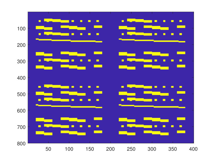 Figure 1
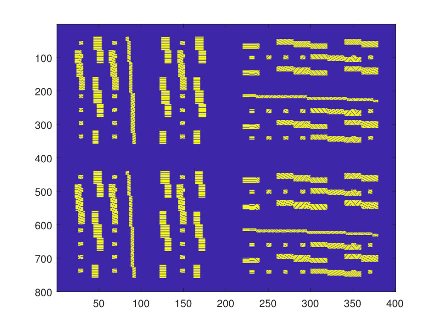 Figure 2
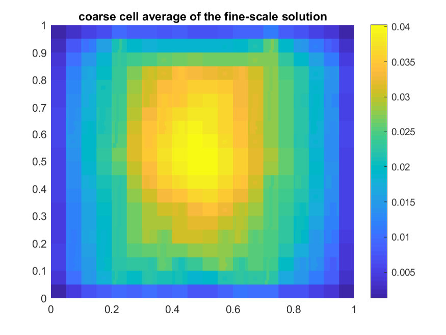 Figure 3
 Figure 4
 Figure 5
 Figure 6
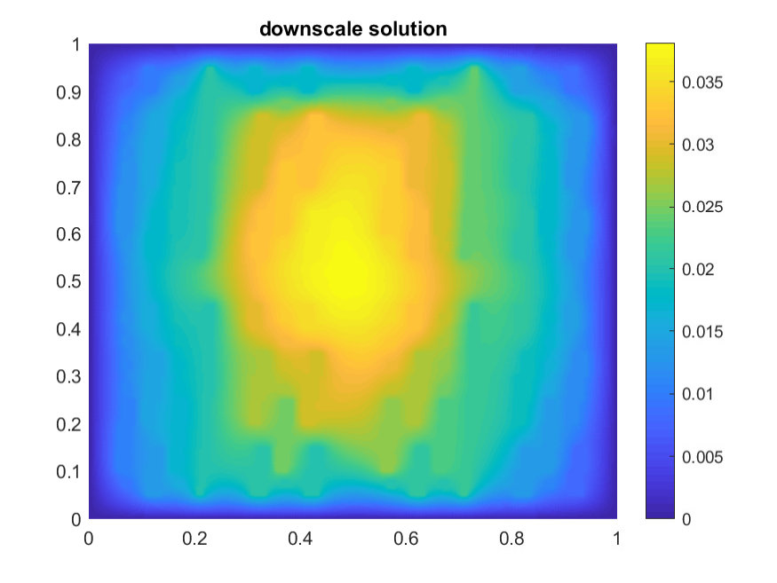 Figure 7
 Figure 8
 Figure 9
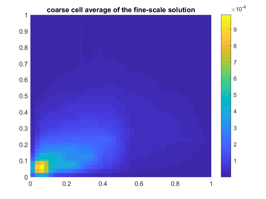 Figure 10
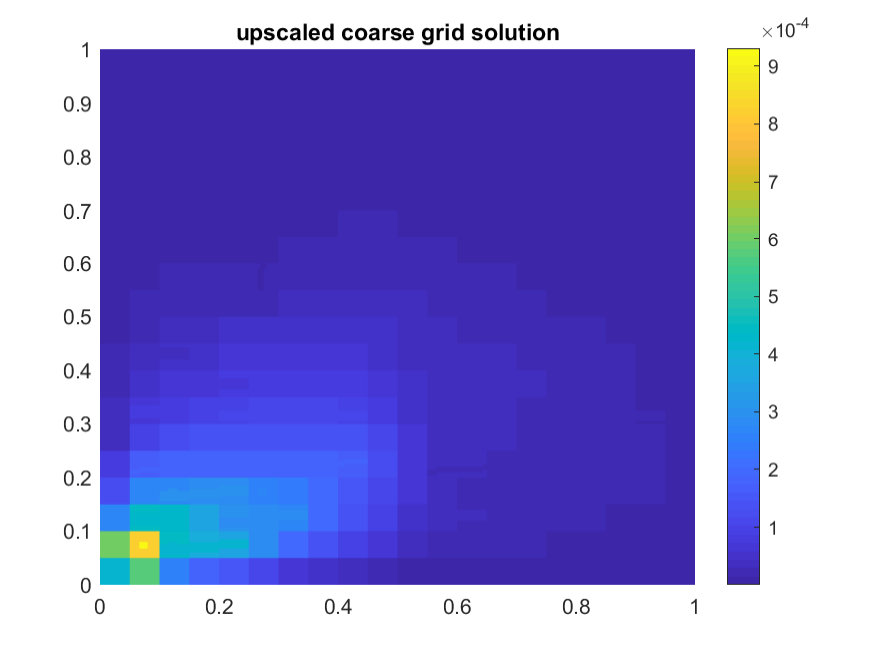 Figure 11
 Figure 12
 Figure 13
 Figure 14
 Figure 15
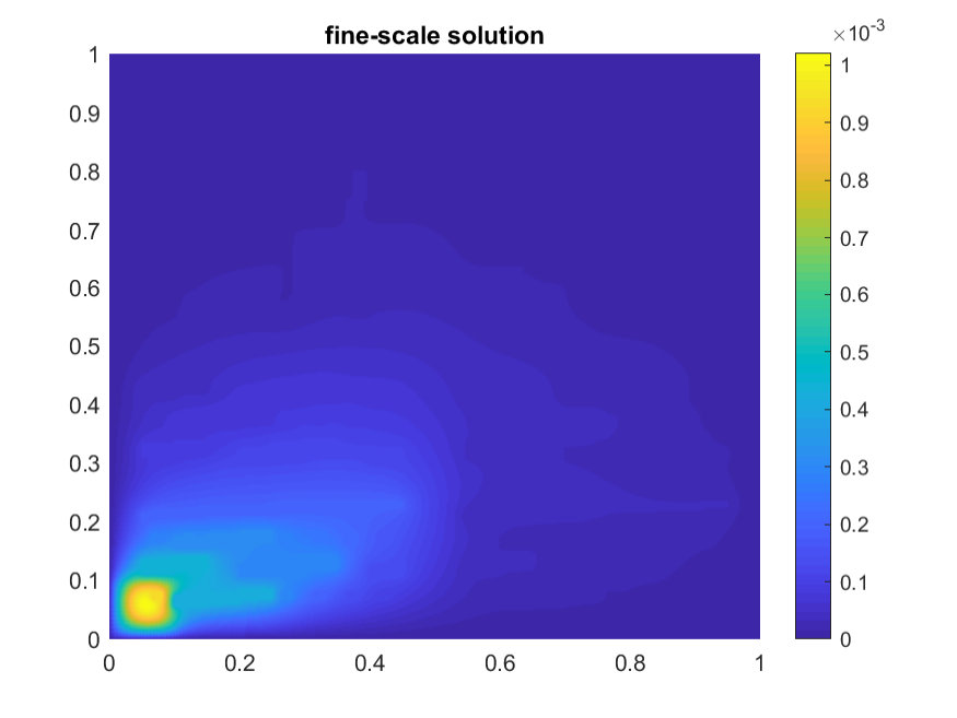 Figure 16
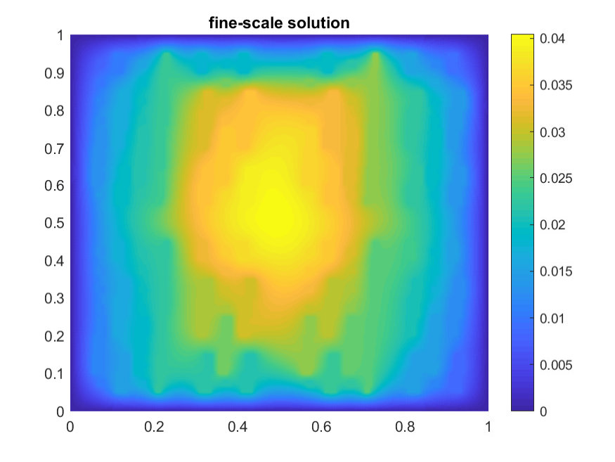 Figure 17
 Figure 18
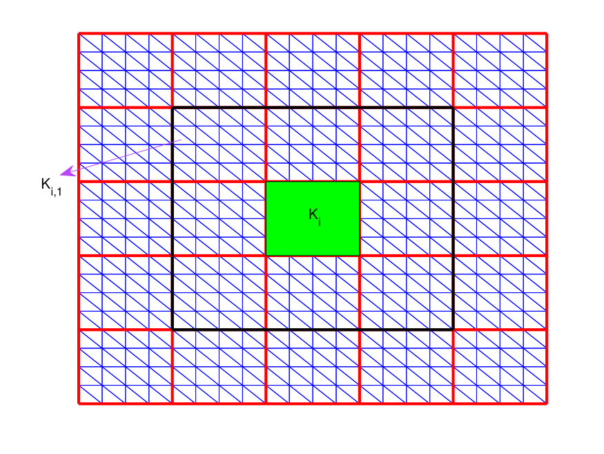 Figure 19
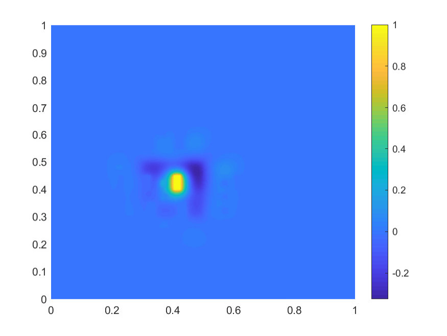 Figure 20
| oversampling coarse layers | ||
|---|---|---|
| 3 | 0.1678 | |
| 4 | 0.0808 | |
| 5 | 0.0453 |
| Layer | coarse mesh 20 20 | coarse mesh 4040 |
|---|---|---|
| 1 | 0.9690 | 0.9876 |
| 3 | 0.4816 | 0.9136 |
| 4 | 0.0808 | 0.4772 |
| 5 | 0.0054 | 0.0453 |
| 6 | 2.759e-4 | 0.0012 |
| Layer Contrast | ||||
|---|---|---|---|---|
| 3 | 0.1575 | 0.4816 | 0.6319 | 0.6526 |
| 4 | 0.0103 | 0.0808 | 0.3796 | 0.6081 |
| 5 | 6.0346e-4 | 0.0054 | 0.0496 | 0.2943 |
| oversampling coarse layers | ||
|---|---|---|
| 3 | 0.0984 | |
| 4 | 0.0382 | |
| 5 | 0.0183 |
| Layer | coarse mesh 20 20 | coarse mesh 4040 |
|---|---|---|
| 1 | 0.8246 | 0.8429 |
| 3 | 0.3070 | 0.7229 |
| 4 | 0.0382 | 0.2408 |
| 5 | 0.0025 | 0.0183 |
| 6 | 1.2742e-4 | 5.337e-4 |
Peer Reviews
No public reviews on file for this paper yet. If you reviewed it on a platform where reviews are public (OpenReview, ICLR, NeurIPS, ICML), you can paste yours below so the community can read it here.
Videos
No videos yet. Explain this paper in a talk, walkthrough, or lecture? Add one.
An analysis of the NLMC upscaling method for high contrast problems
Lina Zhao111Department of Mathematics,The Chinese University of Hong Kong, Hong Kong Special Administrative Region. ([email protected]) Eric T. Chung222Department of Mathematics,The Chinese University of Hong Kong, Hong Kong Special Administrative Region. ([email protected])
Abstract: In this paper we propose simple multiscale basis functions with constraint energy minimization to solve elliptic problems with high contrast medium. Our methodology is based on the recently developed non-local multicontinuum method (NLMC). The main ingredient of the method is the construction of suitable local basis functions with the capability of capturing multiscale features and non-local effects. In our method, each coarse block is decomposed into various regions according to the contrast ratio, and we require that the contrast ratio should be relatively small within each region. The basis functions are constructed by solving a local problem defined on the oversampling domains and they have mean value one on the chosen region and zero mean otherwise. Numerical analysis shows that the resulting basis functions can be localizable and have a decay property. The convergence of the multiscale solution is also proved. Finally, some numerical experiments are carried out to illustrate the performances of the proposed method. They show that the proposed method can solve problem with high contrast medium efficiently. In particular, if the oversampling size is large enough, then we can achieve the desired error.
Keywords: Contraint energy minimization, Upscaling, Non-local multicontinuum method, High contrast
1 Introduction
In this paper we consider
[TABLE]
where is the computational domain and is a high contrast with and is a multiscale field. The proposed method can be extended to 3D easily.
If the coefficient is rough, then the solution to (1.1) will also be rough; to be specific, will not in general be in and may not be in for any . For this kind of low regularity, standard analysis usually fails. Moreover, the classical polynomial based finite element methods could perform arbitrary badly for such problems, see, e.g., [4]. To resolve this issue, various numerical methods have been proposed and analyzed, and among all the methods we mention in particular the special finite element methods [2, 3], the upscaled models [12, 30] and the multiscale methods [20, 18, 21, 19, 1, 10, 7, 6, 23, 24, 16, 17].
The concept of non-local upscaling has been successfully applied to problems in porous media, see, e.g., [14, 11, 13]. Motivated by the work given in [15], the nonlocal multicontinua (NLMC) upscaling technique was initially introduced for flows in heterogeneous fractured media in [9], and have been successfully applied to different problems under application [25, 26, 27, 28]. The main idea of NLMC upscaling technique is to construct the multiscale basis functions over the oversampling domain via an energy minimization principle. Note that the constraint should be chosen properly in order to make the localization possible. One distinctive feature of the method is that it allows a systematic upscaling for processes in the fractured porous media, and provides an effective coarse scale model whose degrees of freedom have physical meaning.
Inspired by the work given in [9, 25, 26], the goal of this paper is to extend the idea of nonlocal multicontinua to problem (1.1). For our approach, we start with decomposing the coarse block into different regions and the criterion used for the decomposition is to have relatively small contrast ratio within each region. Then, we define the constraint energy minimzation problem in the oversampling domain, where the restriction for the basis functions is defined such that they have mean value one in the chosen region and zero mean otherwise, in addition the basis functions vanish on the boundary of the oversampling domain. We remark that the vanishing property is important for the localization of the multiscale basis functions and the localization idea has also been exploited in [22] to solve problems with heterogeneous and highly varying coefficients. Next, we can solve the local minimization problem by using the equivalent saddle point formulation to achieve the multiscale basis functions. The resulting multiscale basis functions have decay property, in addition, it can capture the fine-grid information well provided proper number of overampling layers are chosen. With the multiscale basis functions, we can solve the upscaled equation to obtain the upscaled coarse grid solution. It is worth mentioning that in our method the number of basis function is relatively small and it is equal to the number of scales over the domain. We also analyze the convergence of the proposed method. For this, we first compare the difference between the multiscale basis functions and the global basis functions, combining this with the convergence of the global solution, then we can prove the convergence of the multiscale solution in norm and weighted energy norm. The analysis indicates that the convergence rate only depends on the local contrast ratio, namely, the contrast ratio within each region. With proper number of oversampling layers, the first order convergence measured in energy norm can be obtained. Some numerical experiments are also carried out. The numerical experiments show that with the fixed coarse mesh size, the oversampling layers should be selected properly to achieve the desired error, in addition, for a fixed oversampling size, the performance of the scheme will deteriorate as the medium contrast increases.
The rest of the paper is organized as follows. In the next section, we present the construction of the proposed method for (1.1). The convergence analysis for the multiscale solution is proposed in Section 3. Then, some numerical experiments are investigated in Section 4 to confirm the theoretical results. Finally, the conclusions are given in Section 5.
2 Preliminaries
2.1 Description of NLMC method
The solution of (1.1) satisfies
[TABLE]
where .
Next, the notations of the fine grids and coarse grids are introduced. Let be a coarse-grid of the domain and be a conforming fine triangulation of . We assume that is a refinement of , where and represent the fine and coarse mesh sizes, respectively. Let be the -th coarse block and let be the corresponding oversampled region obtained by enlarging the coarse block by coarse grid layers (See Figure 1 for an illustration). We let be the number of elements in . Furthermore, each coarse block is decomposed into different regions and is the number of regions within coarse block . In addition, we require that within each region , should satisfy and the contrast ratio should be relatively small. In addition, we define for any . We remark that each region is a continuum.
Consider an oversampling region of the coarse block , then the multiscale basis function is constructed by minimizing subject to the following conditions
[TABLE]
where is the Dirac delta function and denotes the area of . We can see that has mean value on the -th region within the coarse block and [math] mean in other regions inside the oversampling domain.
We remark that the above minimization problem is implicit, to solve it explicitly, we can write down the following equivalent variational formulation over each :
[TABLE]
where and is a piecewise constant function with respect to each region of , and denotes restricted to . An illustration of the multiscale basis functions can be found in Figure 2.
Then we obtain our multiscale space
[TABLE]
The resulting coarse grid equation can be written as
[TABLE]
The construction of the local multiscale basis function is motivated by the global basis construction as defined below, and in the subsequent analysis we will exploit the global basis functions to show the convergence analysis. The global basis function is defined by
[TABLE]
Out multiscale finite element space is defined by
[TABLE]
For later analysis, we define to be the projection which is defined for each region as
[TABLE]
and
[TABLE]
In addition, we define as the null space of the projection , namely, . Then for any , we have
[TABLE]
We remark that and interested readers can refer to [8] for the explanations.
The approximate solution obtained in the global multiscale space is defined by
[TABLE]
For later analysis, we define . In addition, for a given subdomain , we define the local -norm by .
2.2 Computational issue
For the convenience of the readers, we write down the implementation of the proposed method as follows.
Calculate the multiscale basis functions by solving (2.2)-(2.3) for each region . 2. 2.
Generate the projection matrix
[TABLE]
where is a column vector using its representation in the fine grid. 3. 3.
Construct the coarse grid system
[TABLE]
and solve the above equation to get .
Note that the downscale solution can be defined by . Our coarse grid solutions have physical meaning, which is the average value of the solution on each region .
3 Error analysis
In this section, we will carry out the error analysis for the proposed method. We first show the convergence of the global basis function defined in (2.4), then we show the decay property of the local multiscale basis function, using which the convergence of the multiscale solution can be obtained.
3.1 Convergence
This subsection presents the convergence of the approximate solution obtained in (2.1) as stated in the next lemma.
Lemma 3.1**.**
Let be the solution in (2.1) and be the solution in (2.5), then we have
[TABLE]
Proof.
By the definitions of and , we have
[TABLE]
Combining these two equations, we can get
[TABLE]
So, we have . It then follows that
[TABLE]
Since , the Poincaré inequality yields
[TABLE]
Therefore, the preceding arguments reveal that
[TABLE]
which gives the desired estimate.
∎
3.2 Decay property of the multiscale basis functions
This section aims to proving the global basis functions are localizable. To this end, for each coarse block , we define to be a bubble function and , where is barycentric coordinates and denotes the fine grids restricted to , and more information regarding the bubble function can be found in [29].
The next lemma considers the following minimization problem defined on a coarse block :
[TABLE]
for a given .
Lemma 3.2**.**
For all , there exists a function such that
[TABLE]
Proof.
Let . The minimization problem is equivalent to the following variational problem: find and such that
[TABLE]
Let . Note that, by the mixed finite element theory (cf. [5]), the well-posedness of the minimization problem is equivalent to the existence of a function such that
[TABLE]
Note that is supported in . We let . By the definition of , we have
[TABLE]
In addition,
[TABLE]
Thus
[TABLE]
and the minimization problem (3.1) has a unique solution . Therefore, and satisfy (3.2)-(3.3). From (3.3), we can obtain . The assertion follows.
∎
The rest of this section attempts to estimating the difference between the global and multiscale basis functions. For this purpose, we first introduce some notations used for the subsequent analysis. We define the cutoff function with respect to these oversampling domains. For each , we recall that is the oversampling coarse region by enlarging by coarse grid layers. For , we define such that and
[TABLE]
Note that we have and are the standard multiscale finite element (MsFEM) basis functions (cf. [18]).
The next lemma shows the difference between the global and multiscale basis functions, which will play an important role in the proof of the convergence of the multiscale solution.
Lemma 3.3**.**
We consider the oversampled domain with . That is, is an oversampled region by enlarging by grid layers. Let be the Dirac delta function. We let be the multiscale basis functions obtained in (2.2)-(2.3) and let be the global multiscale basis functions obtained in (2.4). Then we have
[TABLE]
and
[TABLE]
Proof.
For the given , by Lemma 3.2, there exists a such that
[TABLE]
We let , then we have . Therefore, . We see that and satisfy
[TABLE]
and
[TABLE]
for some , . Subtracting the above two equations and restricting , we have
[TABLE]
Here, we have . Therefore, for , we can get
[TABLE]
where . Thus, we obtain
[TABLE]
Now, we will estimate . We consider the th coarse block . For this block, we consider two oversampled regions and . Using these two overampled regions, we define the cutoff function with the properties in (3.4)-(3.5), where we take and . For any coarse block by (3.4), we have on . Since , we have
[TABLE]
From the above result and the fact that in , we have
[TABLE]
By Lemma 3.2, for the function , there is such that and . Moreover, it also follows from Lemma 3.2, the definition of and the Cauchy-Schwarz inequality that
[TABLE]
Hence, taking in (3.10), we can obtain
[TABLE]
Next, we will estimate the two terms on the right hand side of (3.12).
Step 1: We first estimate the first term in (3.12). By a direct computation, we have
[TABLE]
Note that, we have . For the second term on the righ hand side of the above inequality, we will use the fact that and the Poincaré inequality
[TABLE]
We will estimate the right hand side in Step 3.
Step 2: We will estimate the second term on the right hand side of (3.12). By (3.11), the fact that and the Poincaré inequality, we have
[TABLE]
Combining Steps 1 and 2, we obtain
[TABLE]
Step 3: Finally, we will estimate the term . We will first show that the following recursive inequality holds
[TABLE]
where . Using (3.14) in (3.13), we can get
[TABLE]
By using (3.14) again in (3.15), we can obtain
[TABLE]
By employing the definition of , the energy minimizing property of and Lemma 3.2, we have
[TABLE]
Step 4: We will prove the estimate (3.14). Let . Then we see that in and otherwise. Then we have
[TABLE]
We estimate the first term in (3.16). For the function , using Lemma 3.2, there exists such that and . For any coarse elements , since on , we have for any
[TABLE]
On the other hand, since in , we have
[TABLE]
From the above two conditions, we see that and consequently . Note that, since , we have . We also note that . By (3.7), the functions and have disjoint supports, so . Then, by the definition of , we have
[TABLE]
By the construction of , we have . Then we can estimate the first term in (3.16) by the Cauchy-Schwarz inequality and Lemma 3.2
[TABLE]
For all coarse elements and assume that within , since , we have from the Poincaré inequality that
[TABLE]
Summing the above over all coarse elements , we have
[TABLE]
To estimate the second term in (3.16), we have from the Poincaré inequality
[TABLE]
Hence, the preceding arguments yield the upper bound for (3.16)
[TABLE]
Thus
[TABLE]
∎
Lemma 3.4**.**
With the same assumptions as in Lemma 3.3, we can obtain
[TABLE]
Proof.
Let . By the constructions in (2.2)-(2.3) and (2.4) and Lemma 3.2, there is such that
[TABLE]
It then follows from (3.8) and (3.9) that
[TABLE]
Putting in (3.17), we can obtain
[TABLE]
Thus
[TABLE]
For each , we have
[TABLE]
In addition, since for all with , we can get
[TABLE]
which yields the desired estimate by combining with (3.18).
∎
The convergence of the multiscale solution can be stated in the next theorem.
Theorem 3.1**.**
Let be the solution of (2.1) and be the multiscale solution, then we have
[TABLE]
Moreover, if , then we have
[TABLE]
Proof.
We write . Then we define . It then follows from the Galerkin orthogonality that
[TABLE]
Lemma 3.4 yields
[TABLE]
The above equation together with Lemma 3.1 and (3.21) implies
[TABLE]
This yields (3.19).
The Poincaré inequality yields
[TABLE]
An application of (2.5) and the Cauchy-Schwarz inequality gives
[TABLE]
Therefore
[TABLE]
Then proceeding analogously to [8] and employing the fact that is relatively small, we can conclude that if , then we can obtain (3.20).
Next, we consider the estimate for . Consider the dual problem
[TABLE]
Then, the Cauchy-Schwarz inequality and (3.20) yield
[TABLE]
Thus
[TABLE]
∎
4 Numerical experiments
This section presents numerical experiments to verify the capability of the proposed method to the problem with high contrast medium. To compare the results, we exploit the relative error between coarse cell average of the fine-scale solution and the upscaled coarse grid solution
[TABLE]
Example 4.1**.**
In this example, we take , on and we set . The medium is shown in Figure 3 and we assume that the fine mesh size to be , That is, the medium has a resolution. We consider the contrast of the medium is where the value of is large in the yellow region. For the NLMC method, we consider two continua.
The fine scale and upscaled solutions for coarse mesh with oversampling layers can be found in Figure 4-Figure 5. In Figure 4, we display the downscale and fine scale solution and in Figure 5 we show the upscaled coarse solution and the average value of the fine scale solution. In addition, the numerical results for coarse mesh with 5 oversampling layers are reported in Figure 6-Figure 7. From which we observe very good agreement between the fine-scale solution and the computed upscaled solution.
In Table 1, we present the relative error with varying coarse grid size. With proper choices of oversampling layers, we can see that the error converges. The relative error for coarse grids and , and for different number of oversampling layers are reported in Table 2. From which we can see that for a fixed contrast value, the error decays as the oversampling size increases. In addition, as the number of coarse grid increases, more oversampling layers are required in order to achieve the desired error. Furthermore, for a fixed oversampling size, the performance of the scheme will deteriorate as the medium contrast increases, which can be illustrated by Table 3.
Example 4.2**.**
In this example, we again take and the profile of is shown in Figure 8, where is taken to be some random numbers between for the blue region and is or in the yellow region. For the NLMC method, we consider three continua, namely, , and . In addition, is taken to be
[TABLE]
The fine scale and upscaled solutions for coarse mesh with oversampling layers can be found in Figure 9-Figure 10. In Figure 9, we display the downscale and fine scale solution and in Figure 10 we show the upscaled coarse solution and the average value of the fine scale solution. The numerical results for coarse mesh with 5 oversampling layers are reported in Figure 11-Figure 12. We can observe that the fine-grid solution and the upscaled coarse grid solution match well.
Then in Table 4 we display the relative error with respect to different coarse mesh sizes. With proper number of oversampling layers, the error converges as reported in Example 4.1. Next, the relative error for coarse grids and with respect to different number of overampling layers are also reported in Table 5, and this example once again highlights that the error decays as the oversampling layers increase, in addition, more oversampling layers are needed to obtain the desired error as the coarse mesh size decreases.
5 Conclusion
In this paper we have developed a simple constraint energy minimization on the oversampling domain to generate the multiscale basis functions, where the construction of the multiscale basis functions relies on the scale separation. In addition, our theory illustrates that the number of oversampling layers required for the convergence is related to the local contrast ratio and the coarse mesh size . Small contrast ratio in each region guarantees the convergence, thus, one should define proper regions in the numerical experiments in order to achieve the desired convergence. Two numerical examples are carried out to test the performances of the proposed method. The numerical results indicate that the relative error decays as the number of oversampling layers increases for a fixed coarse mesh size, furthermore, for a fixed oversampling size, the performance of the scheme will deteriorate as the medium contrast increases.
Acknowledgements
The research of Eric Chung is partially supported by the Hong Kong RGC General Research Fund (Project numbers 14304217 and 14302018) and CUHK Faculty of Science Direct Grant 2017-18.
The reference list from the paper itself. Each links out to its DOI / PubMed record.
- 1[1] T. Arbogast, G. Pencheva, M. F. Wheeler, and I. Yotov , A multiscale mortar mixed finite element method , Multiscale Model. Simul., 6 (2007), pp. 319–346.
- 2[2] I. Babus̆ka and J. E. Osborn , Generalized finite element methods: their performance and their relation to mixed methods , SIAM J. Numer. Anal., 20 (1983), pp. 510–536.
- 3[3] I. Babus̆ka, G. Caloz, and J. E. Osborn , Special finite element methods for a class of second order elliptic problems with rough coefficients , SIAM J. Numer. Anal., 31 (1994), pp. 945–981.
- 4[4] I. Babus̆ka , Can a finite element method perform arbitrarily badly? , Math. Comp., 69 (2000), pp. 443–462.
- 5[5] F. Brezzi and M. Fortin , Mixed and hybrid finite element methods , Springer-Verlag, New York, 1991.
- 6[6] E. Chung, Y. Efendiev and T. Y. Hou , Adaptive multiscale model reduction with generalized multiscale finite element methods , J. Comput. Phys., 320 (2016), pp. 69–95.
- 7[7] E. T. Chung, Y. Efendiev, and W. Leung , An adaptive generalized multiscale discontinuous Galerkin method for high-contrast flow problems , Multiscale Model. Simul., 16 (2018), pp. 1227–1257.
- 8[8] E. T. Chung, Y. Efendiev, and W. Leung , Constraint energy minimizing generalized multiscale finite element method , Comput. Methods Appl. Mech. Engrg., 339 (2018), pp. 208–319.