Mechanics-Aware Modeling of Cloth Appearance
Zahra Montazeri, Chang Xiao, Yun (Raymond) Fei, Changxi Zheng, and, Shuang Zhao

TL;DR
This paper presents a novel physics-based model that captures how fabric microstructures change under mechanical forces, significantly improving the realism of cloth appearance rendering.
Contribution
It introduces a mechanics-aware cloth appearance model that integrates yarn and fiber-level simulations with a new parameter fitting algorithm and neural network for realistic, dynamic rendering.
Findings
The model produces photorealistic, mechanically plausible cloth appearances.
It effectively captures microstructure changes due to external forces.
The approach enables dynamic cloth rendering with high fidelity.
Abstract
Micro-appearance models have brought unprecedented fidelity and details to cloth rendering. Yet, these models neglect fabric mechanics: when a piece of cloth interacts with the environment, its yarn and fiber arrangement usually changes in response to external contact and tension forces. Since subtle changes of a fabric's microstructures can greatly affect its macroscopic appearance, mechanics-driven appearance variation of fabrics has been a phenomenon that remains to be captured. We introduce a mechanics-aware model that adapts the microstructures of cloth yarns in a physics-based manner. Our technique works on two distinct physical scales: using physics-based simulations of individual yarns, we capture the rearrangement of yarn-level structures in response to external forces. These yarn structures are further enriched to obtain appearance-driving fiber-level details. The…
Click any figure to enlarge with its caption.
 Figure 1
 Figure 2
 Figure 3
 Figure 4
 Figure 5
 Figure 6
 Figure 7
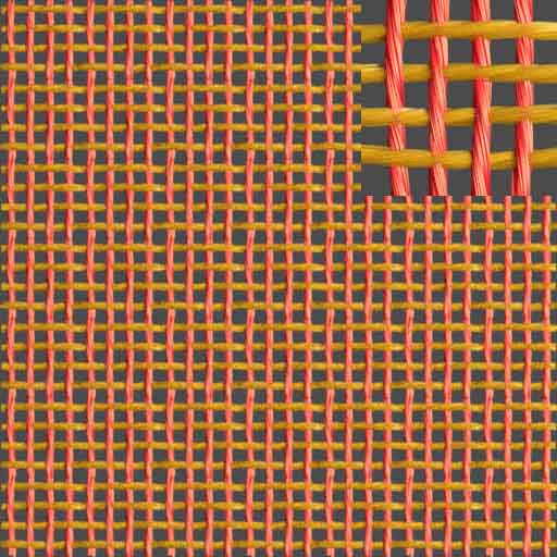 Figure 8
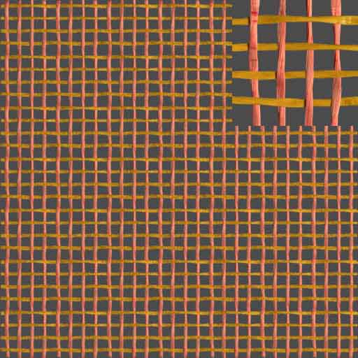 Figure 9
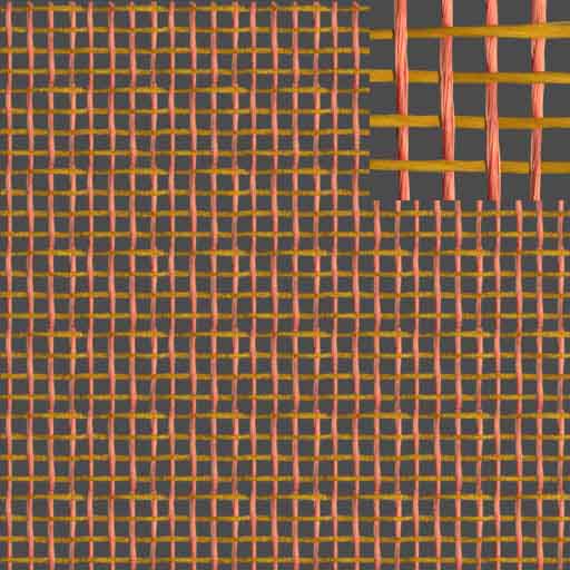 Figure 10
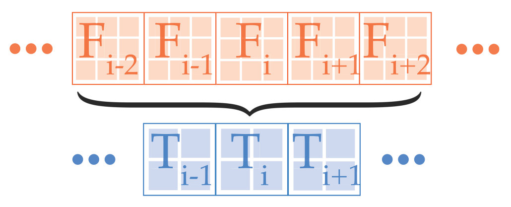 Figure 11
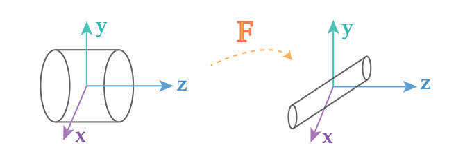 Figure 12
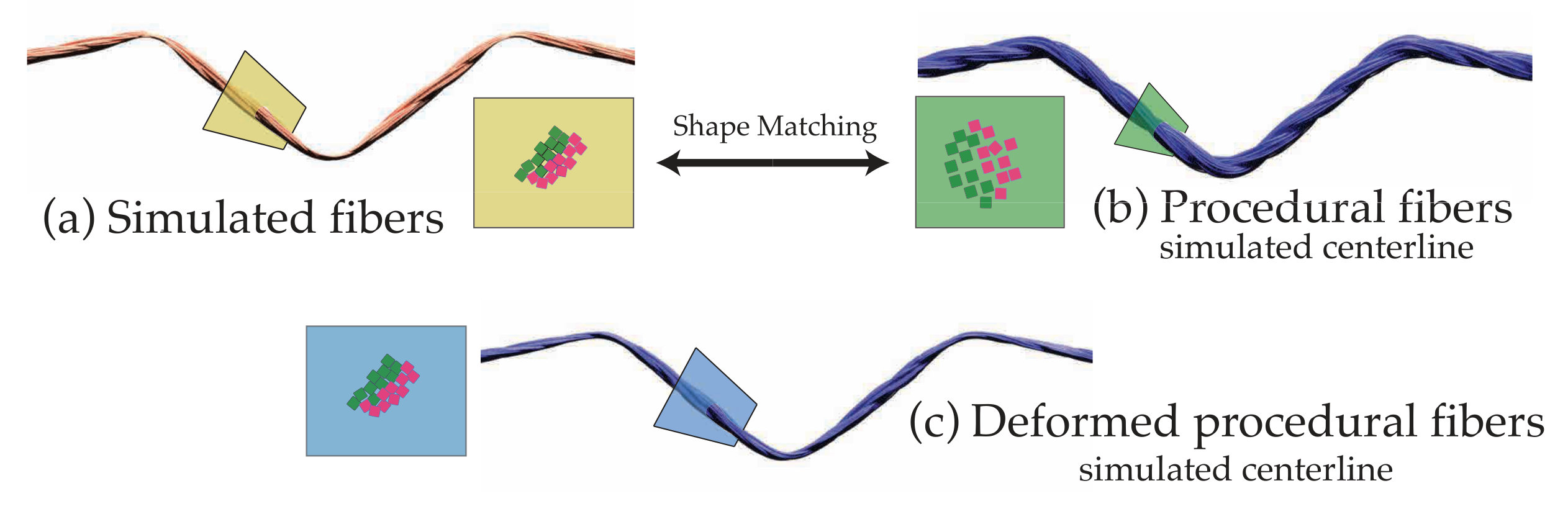 Figure 13
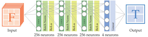 Figure 14
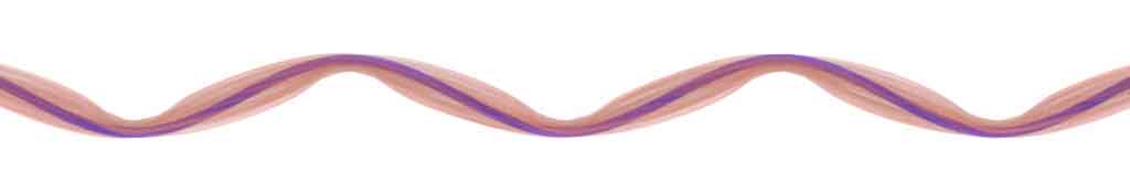 Figure 15
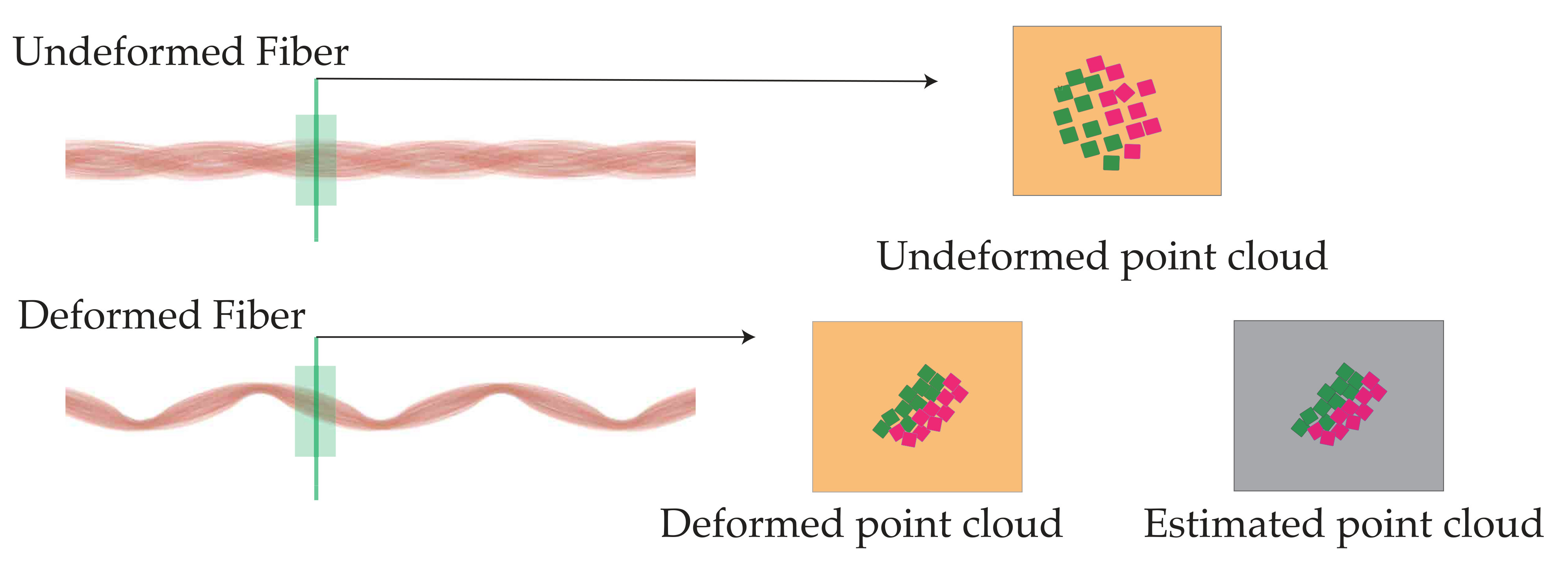 Figure 16
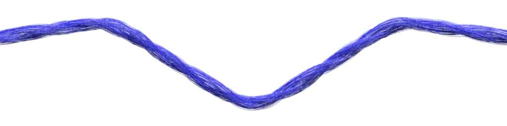 Figure 17
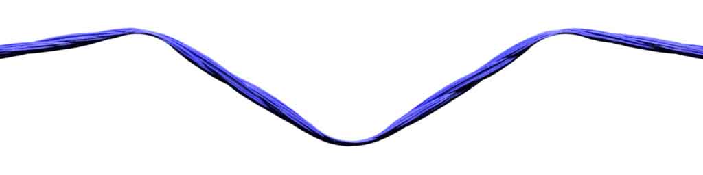 Figure 18
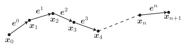 Figure 19
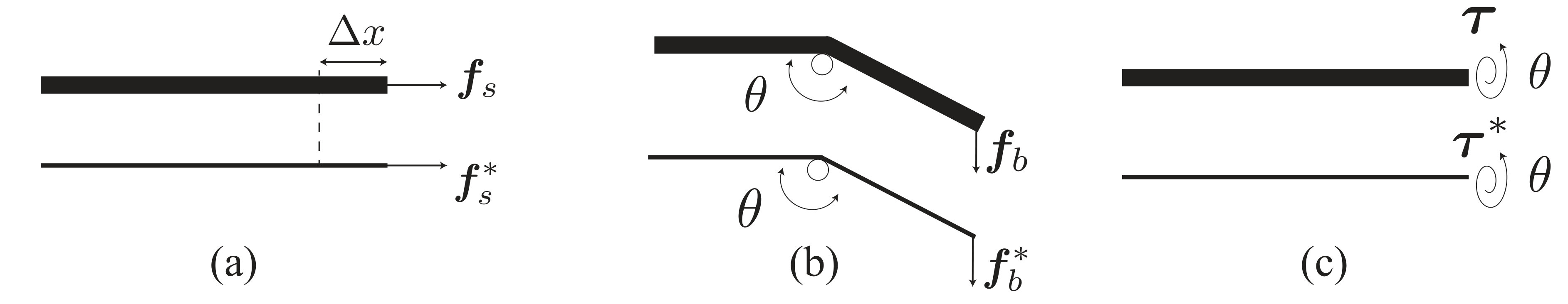 Figure 20
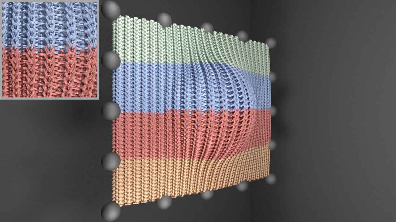 Figure 21
 Figure 22
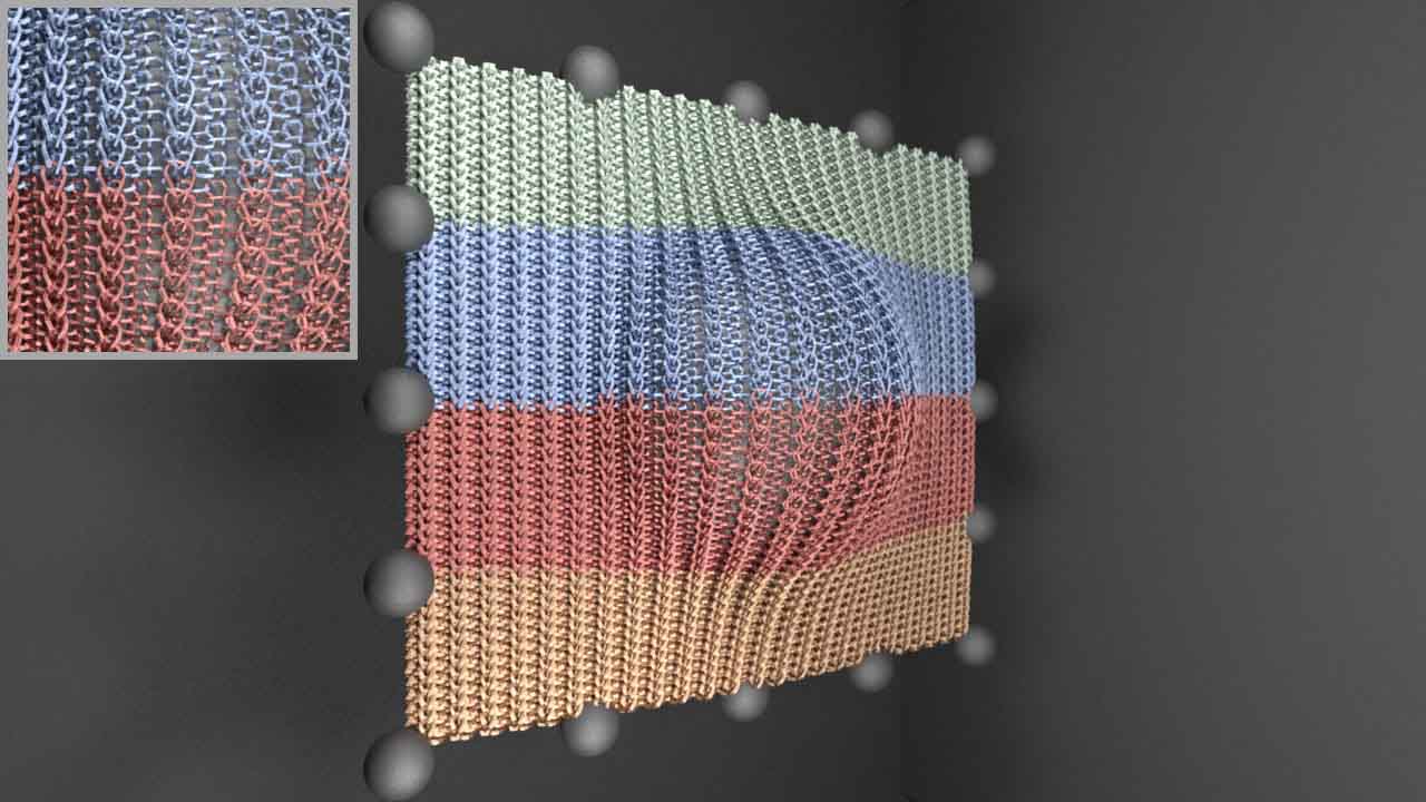 Figure 23
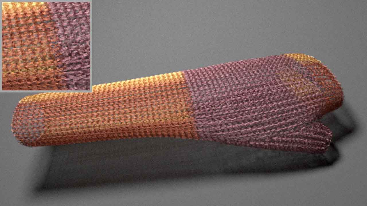 Figure 24
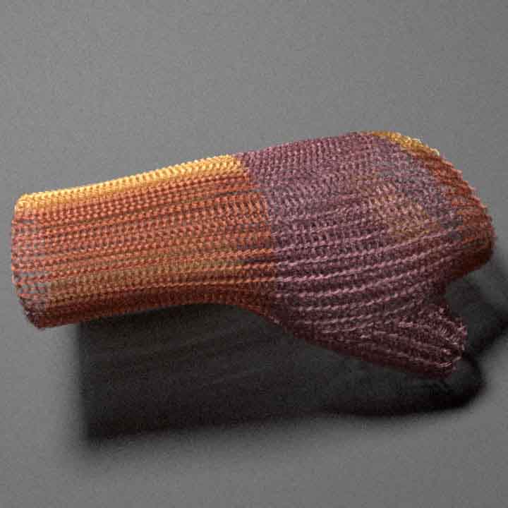 Figure 25
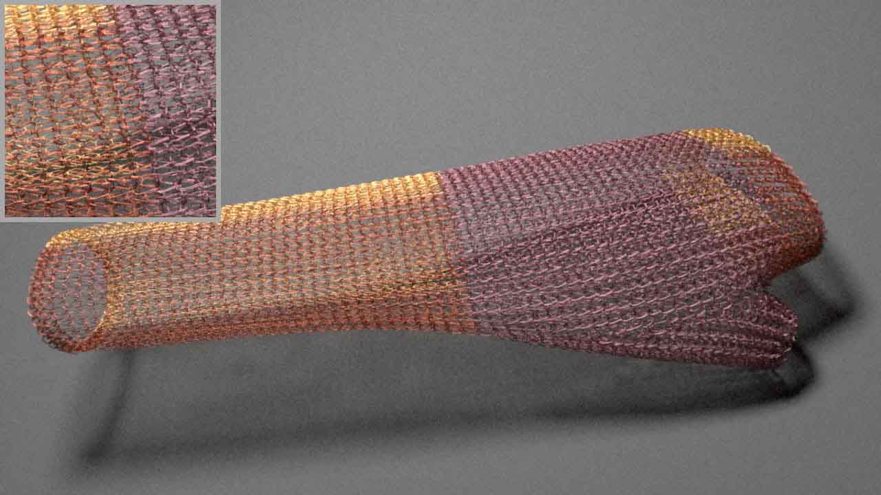 Figure 26
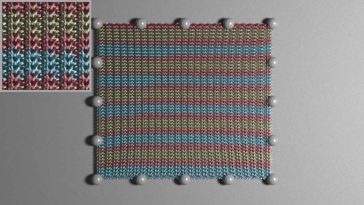 Figure 27
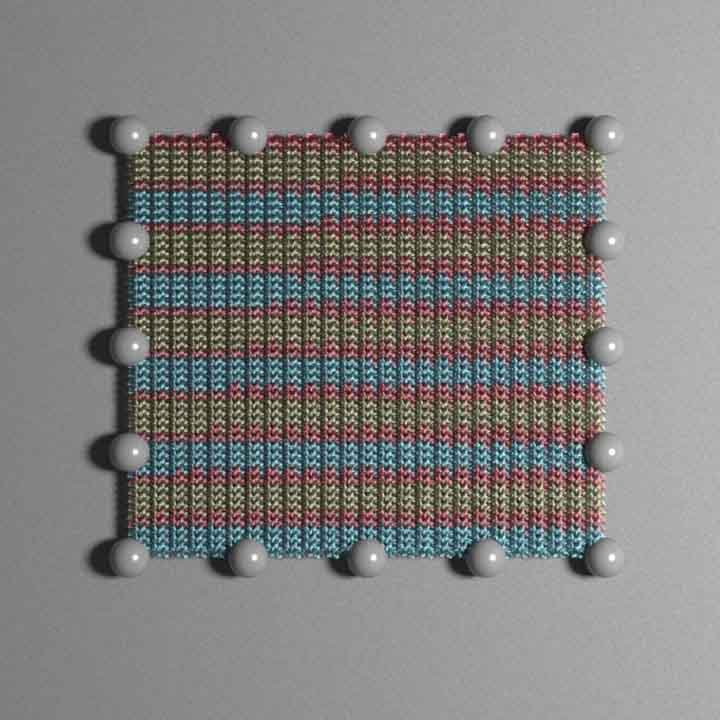 Figure 28
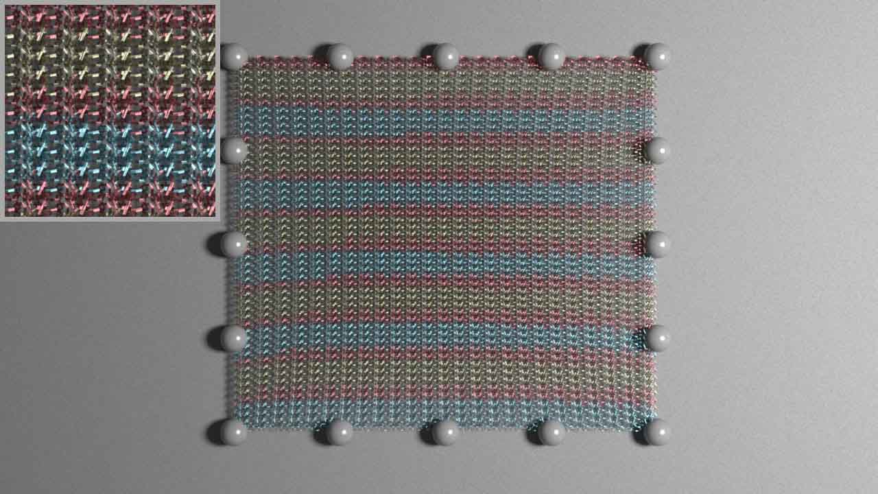 Figure 29
 Figure 30
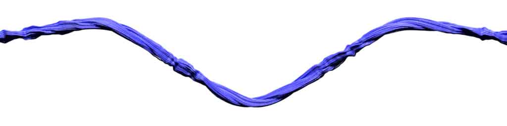 Figure 31
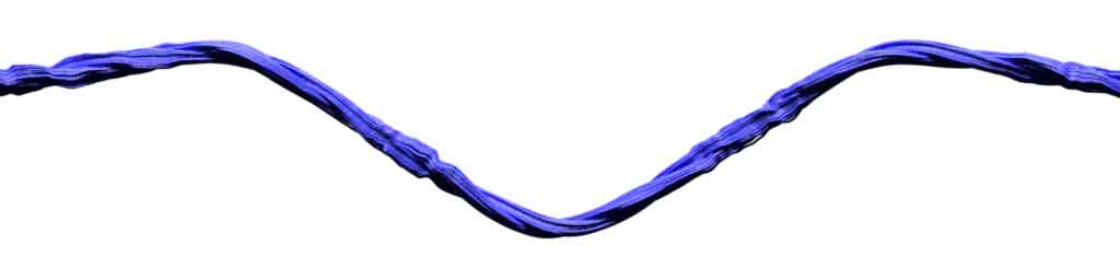 Figure 32
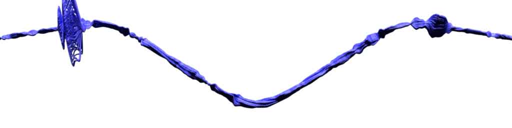 Figure 33
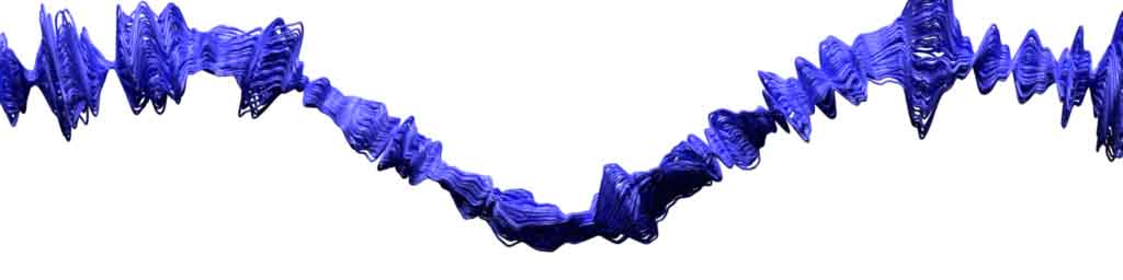 Figure 34
 Figure 35
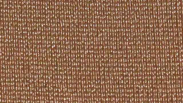 Figure 36
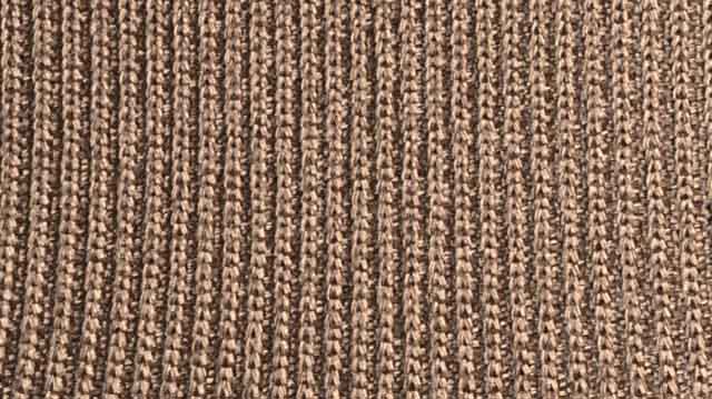 Figure 37
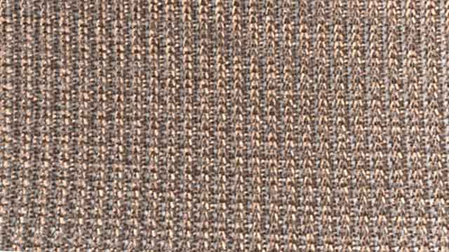 Figure 38
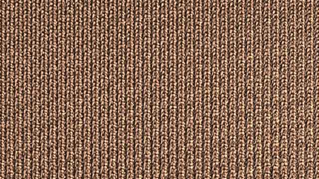 Figure 39
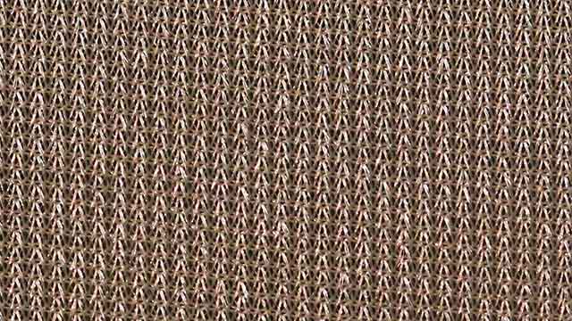 Figure 40
| Param. | Value |
| Scene | # vertices | Fiber-level simulation | Yarn-level simulation | Fiber generation + NN evaluation |
|---|---|---|---|---|
| Figure 13 | 300 | 8 h | 15 min | 20 sec |
| Figure 17-a | 85832 | - | 20 h | 1 min |
| Figure 17-b | 85832 | - | 18 h | 30 sec |
| Figure 17-c | 58545 | - | 28 h | 1 min |
| Figure 18-a | 100000 | - | 9 h | 1 min |
| Figure 18-b | 100000 | - | 10 h | 1 min |
| Figure 18-c | 1266000 | - | 110 h | 10 min |
Peer Reviews
No public reviews on file for this paper yet. If you reviewed it on a platform where reviews are public (OpenReview, ICLR, NeurIPS, ICML), you can paste yours below so the community can read it here.
Videos
No videos yet. Explain this paper in a talk, walkthrough, or lecture? Add one.
Mechanics-Aware Modeling
of Cloth Appearance
Zahra Montazeri, Chang Xiao, Yun (Raymond) Fei, Changxi Zheng, and Shuang Zhao
Zahra Montazeri, Chang Xiao, Yun (Raymond) Fei, Changxi Zheng, and Shuang Zhao Z. Montazeri and S. Zhao was with the Department of Computer Science, University of California, Irvine, CA, 92697.
E-mail: [email protected] C. Xiao, Y. (R.) Fei and C. Zheng are with Columbia University, New York, NY, 10027Manuscript received May 12, 2019; revised May 12, 2019.
Abstract
Micro-appearance models have brought unprecedented fidelity and details to cloth rendering. Yet, these models neglect fabric mechanics: when a piece of cloth interacts with the environment, its yarn and fiber arrangement usually changes in response to external contact and tension forces. Since subtle changes of a fabric’s microstructures can greatly affect its macroscopic appearance, mechanics-driven appearance variation of fabrics has been a phenomenon that remains to be captured.
We introduce a mechanics-aware model that adapts the microstructures of cloth yarns in a physics-based manner. Our technique works on two distinct physical scales: using physics-based simulations of individual yarns, we capture the rearrangement of yarn-level structures in response to external forces. These yarn structures are further enriched to obtain appearance-driving fiber-level details. The cross-scale enrichment is made practical through a new parameter fitting algorithm for simulation, an augmented procedural yarn model coupled with a custom-design regression neural network. We train the network using a dataset generated by joint simulations at both the yarn and the fiber levels. Through several examples, we demonstrate that our model is capable of synthesizing photorealistic cloth appearance in a mechanically plausible way.
Index Terms:
Cloth appearance, cloth mechanics
1 Introduction
It is a universal phenomenon that a material’s microstructure affects its macroscopic appearance profoundly. In light of this, computer graphics has made significant advances toward capturing realistic object appearance by modeling its microstructures (e.g., [9, 16, 10, 23]). Motivated by its utter prominence in virtual senses, cloth appearance has also been modeled microscopically. State-of-the-art micro-appearance models [33, 20, 35] can produce cloth renderings with stunning richness and details, by accounting for the fabric’s micro-geometric structures (i.e., the arrangement of fibers and yarns).
We argue that the microstructures of cloth should be modeled not only geometrically but also mechanically. This is because the appearance-driving arrangement of a fabric’s constituent fibers and yarns is by no means fixed. For instance, a simple stretch of a piece of fabric may thin its yarns, making the fabric more see-through and changing its shininess (see Figure 2). Even without external distortion, the interaction between individual yarns of a cloth can change yarn shapes and cause specific texture patterns to emerge [18, 8]. The mechanical response—the interplay between small-scale filament structures and their material properties—plays a significant role in a fabric’s appearance.
From this vantage point, we introduce a cloth appearance model that incorporates mechanical responses of a fabric’s microstructures for better capturing the fabric appearance and its changes under external forces.
A seemingly straightforward idea is to rely on physics-based simulation to reconfigure the structures of yarns and fibers. However, executing this idea needs to address a significant computational challenge. On the one hand, it has been shown that both the structure of fibers (i.e., how the individual filaments form a yarn) and the structure of yarns (i.e., how the individual yarns are interwoven) are instrumental for fabric appearance [33, 20, 27, 35, 6]. On the other hand, while there exist physics-based models that simulate individual yarns of a cloth [19, 8], simulating individual fibers is intractable, because even for a sizable cloth, a myriad of fibers must be included.
We tackle this challenge through a bi-scale approach: we simulate the cloth only at the yarn level and synthesize the fiber-level details in a mechanics-aware manner during post-processing. The synthesis of fibers is enabled by augmenting the procedural yarn model [27, 35] with spatially varying parameters derived from the simulated yarn states. These parameters are used to deform the procedurally generated fibers in the way that reflect the fabric’s mechanical response. Since the relationship between the fiber-deforming parameters and the simulated yarn-level states is highly complex, we leverage a custom-design regression neural network to learn this relation.
The training dataset of our regression network is generated by running physics-based simulations at both the yarn level (where a cloth yarn is modeled as a single curve) and the fiber level (where a yarn is depicted as a bundle of fiber curves). To make the training simulations tractable, we design the neural network such that they involve only a small yarn segment. Furthermore, to ensure the consistency between the simulations at both scales, we develop a new parameter fitting algorithm that automatically determines the (homogenized) material properties at the yarn level using those from the fiber level.
At runtime, our method simulates the microstructures of a fabric at the yarn level. It then utilizes procedural yarn modeling coupled with the pre-trained regression network to generate the fabric’s fiber-level geometries and adapt them to the simulated yarn states. In this way, we are able to produce diverse and physically plausible fabric appearance (Figure 1).
To our knowledge, this is the first mechanics-aware technique for modeling the appearance of cloth (or any material if that matters): existing techniques offering fiber-level details either rely on measured fiber geometries that are virtually impossible to animate [33, 20], or use procedurally generated fibers with fiber and yarn mechanics completely neglected [27, 35, 24]. Our technique is also independent of the underlying cloth simulation method: although we choose to use a state-of-the-art offline approach for maximized accuracy, other yarn-level simulation approach can be readily used as well. Our major technical contributions include:
- •
A parameter homogenization technique that fits yarn-level mechanical parameters so that yarn centerlines match between fiber-level and yarn-level simulations.
- •
A custom-design regression neural network that learns the mapping from simulated yarn-level states to fiber-deforming parameters.
We validate our method by comparing fiber-level simulations and photographs (Figures 13 and 16). To demonstrate the use of our method, we apply it to a few fabrics under various mechanical deformations, and show their appearance changes in response to the interaction with the environment (Figures 1, 17, and 18).
2 Related Work
Cloth appearance models
Modeling and reproducing the appearance of a cloth has been an active research area in computer graphics for decades. Traditionally, cloth are modeled as 2D thin sheets with the appearance described using generic [30, 2, 31] or specialized surface reflectance models [1, 15, 26]. These models offer adequate quality for reproducing cloth appearance when viewed from a distance where individual cloth yarns are barely visible. On the other hand, they lack the fidelity and details to produce plausible close-up renderings and the generality to capture fabrics’ diverse visual effects (such as strong textures and grazing-angle highlights) usually arising from their characteristic microstructures.
Recently, a family of micro-appearance models has been introduced to model fabric appearance [33, 34, 27, 20, 35, 32, 6, 24, 21]. Unlike earlier methods, these techniques explicitly model fabrics’ fiber-level microstructures using high-resolution volumes or fiber meshes. Since these microstructures largely affect a fabric’s overall appearance, micro-appearance models enjoy the unprecedented details and the generality to capture the appearance of a wide variety of fabrics.
Unfortunately, these models are mechanically agnostic: many of them rely on measured microstructures that cannot be mechanically deformed at all [33, 34, 20, 21]; others use specialized procedures that completely neglect fiber mechanics [27, 35, 32, 24], producing inaccurate overall appearance (e.g., see Figure 2). In short, these models are significantly limited when modeling animated fabrics.
Cloth and yarn simulation
Computer graphics has also seen a long history of simulating cloth and yarns. A thorough review can be found in the survey [29]. Oftentimes, a piece of cloth is modeled as a 2D surface, discretized with a triangular or quadrilateral mesh [3, 13]. Since a real cloth is woven by a set of fiber bundles (or yarns), a more faithful method is to model those yarns directly. The first of such models was introduced by Kaldor et al. [18], and later accelerated in [19].
The main challenge of simulating at yarn level is the high cost of resolving contacts. To address this issue, Cirio et al. [8] introduced sliding constraints to efficiently treat inter-yarn contacts. Our work is built on a Lagrangian/Eulerian approach of resolving contacts [17]. Extending the material point method [28], this approach represents yarns as polylines embedded in a background Eulerian grid, and resolves collisions by modeling them as volumetric deformations. In the same framework, this method can also simulate thin shells, while ignoring bending and twisting forces. This limitation is addressed recently for mesh-based thin shells [14]. We address this limitation for simulating individual yarns by incorporating the elastic rod model [4], similar to the recent work by Fei et al. [11].
Despite of these advances, simulating individual fibers in a sizable cloth remains intractable, because an excessively large number of fibers is needed. While Jiang et al. [17] managed to simulate multiple “threads” per yarn in their examples, the number of threads is still much smaller than the typical number of fibers in a real yarn. In this work, we sidestep the challenge of simulating fibers fully. Our simulation still performs at the yarn level, but we design a deep neural network to “upsample” the yarn-level simulation results to obtain fiber-level details.
Cloth rendering vs. simulation
Historically, the research on cloth appearance modeling and physics-based simulation advance largely in parallel, probably because the two lines of research have been traditionally considered from different physical perspectives (optics vs. mechanics). Although cloth simulation results are often demonstrated with realistic rendering, it is very rare, if not at all, that a cloth appearance model has benefited from physics-based simulation. In this work, we show that the two seemingly separated types of models can work in tandem, yielding an improved cloth appearance model.
3 Method Overview
The structure of fabrics is complex at multiple scales. As a whole, a fabric consists of thousands of threads, or yarns, combined via manufacturing techniques like weaving and knitting. Each yarn is, in turn, comprised of tens to hundreds of micron-radius filaments, or fibers. Since a fabric’s yarn and fiber arrangements significantly affects its overall appearance, our goal is to capture cloth’s mechanical response down to the fiber level.
To this end, we leverage physics-based simulation to capture a fabric’s yarn- and fiber-level mechanics. Unfortunately, simulating the dynamics of all fibers in an entire fabric is generally intractable. Instead, we propose to simulate at yarn level (at runtime), and then procedurally generate fibers around simulated yarns in a mechanics-aware manner to complete the appearance model.
To enable mechanics-aware generation of fiber structures, our method consists of three major components:
- •
Training. In our training phase, we simulate a single yarn under a range of conditions at both the yarn and fiber levels. For each pair of simulation results, we compare the simulated fiber curves and procedurally generated ones (guided by the simulated yarn centerline). The discrepancy between the two is learned by a custom-design regression network, one that maps the simulated yarn-level states (i.e., mechanical forces) to the discrepancy-compensating fiber deformations.
- •
Material parameter homogenization. The training step demands consistency between the yarn- and fiber-level simulations. Therefore, given the material properties of individual fibers, we determine their yarn-level counterparts to ensure the consistency between yarn centerlines simulated at both levels (under identical initial conditions). This is achieved by fitting (or homogenizing) yarn-level material parameters using fiber-level simulations.
- •
Runtime. At runtime, we simulate the dynamics of full fabrics only at the yarn level. With individual yarn centerlines and forces along them determined by the simulation, we procedurally generate fibers following these centerlines and use the trained regression network to further adjust the fibers so that they respond to yarn-level forces such as stretching and compression properly.
The pipeline described above is also summarized in Figure 3. In the following sections, we detail our training stage in §4, parameter fitting in §5, and runtime phase in §6.
4 Training Phase
The objective of our training phase is to acquire a mapping between yarn-level deformation and the corresponding fiber reconfiguration. This mapping will be used at run-time to procedurally generate fiber structures in a mechanics-aware manner. To learn the mapping, we simulate a single yarn under a few predetermined configurations at both the yarn and the fiber levels. These training simulations are set up under identical conditions to provide consistent dynamics across both levels.
We will elaborate our simulation models and parameter choices in §5. In this section, we focus on our main training phase. In §4.1, we briefly revisit the procedural approach for generating cloth models with fiber-level details. Then, in §4.2, we show how this procedure can be extended to become mechanics-aware by leveraging a custom-design regression neural network.
4.1 Background: Procedural Modeling of Fiber Geometry
To generate a cloth model with fiber-level details, a procedural approach originated in textile design has been introduced to graphics recently [27, 35]. This approach takes as input a set of yarn centerlines and synthesizes fiber curves around each yarn independently.
For a yarn with its centerline following the -axis, each of the constituent fiber is modeled as a circular helix:
[TABLE]
where , and control the radius, pitch and initial phase of the helix , respectively. When building a procedural yarn, the radius of each fiber is drawn independently from a probability distribution
[TABLE]
where and are two parameters shared by all fibers.
To better model the migration of fibers, Eq. (1) can be extended to allow the helix radius to vary with . A typical implementation of this idea is to have changing under a sinusoidal pattern between two predefined minimal and maximal values. Additionally, real-world yarns usually contain multiple substrands, or plies. In this case, each ply can be described using Eqs. (1, 2). Then, the yarn is formed by twisting all the constituent plies around a common centerline. Please refer to the prior works [27, 35] for more details on fiber migration and multi-ply yarn modeling.
Lastly, given a centerline expressed as a 1D curve parameterized by arc length with normal and binormal , a straight yarn centered at the -axis can be warped to follow this centerline by transforming each fiber to given by
[TABLE]
where and denote the - and -components of , respectively.
4.2 Learning How Fibers Deform
The procedural model outlined in Eqs. (1–3) does not capture the deformation of yarns due to their mechanical responses (e.g., contacting with other yarns and objects or being stretched).
To address this problem, we augment the procedural yarn model with a cross-sectional affine transformation that varies spatially. Specifically, transforms each fiber to:
[TABLE]
which can in turn be warped to follow arbitrary yarn centerlines as before using Eq. (3). Based on this formulation, the mechanics-aware modeling of a fabric’s fiber microstructures boils down to finding proper cross-sectional transformations . This, however, is challenging since cloth fibers usually react to mechanical forces in complicated ways based on their material properties and geometric arrangements.
We aim to obtain the cross-sectional transformations using only results simulated at the yarn level. During these simulations, a yarn is represented as a polyline where each segment is associated with a deformation gradient that describes the local volumetric deformation. We provide more details on physics-based simulation of cloth yarns and fibers in §5.
One naïve approach is to directly use the yarn-level deformation gradients to transform the fibers. Unfortunately, this generally leads to unsatisfactory results, as demonstrated in Figure 4.
We instead leverage a custom-design regression neural network to infer the cross-sectional transformations based on yarn-level deformation gradients . Our goal here is to learn a mapping between the deformation gradients and the cross-sectional deformations so that the latter can be used to deform the procedurally generated fibers via Eq. (4). Since different types of yarns (e.g., cotton vs. silk) generally exhibit distinctive fiber structures that cause the yarns to react to external forces differently, we learn the mapping for each yarn separately.
4.2.1 Training data generation
We generate training data by performing a series of simulations of a single yarn at both the fiber and the yarn levels. To ensure that the training dataset covers a wide range of yarn and fiber deformations driven by mechanical forces, we configure our training simulations to include a single yarn compressed by a few rigid cylinders. We use multiple cylinder arrangements for the simulations (Figure 5), and collect the results as our training dataset.
Training simulations
For each simulation configuration, as shown in Figure 6-a, we use the procedural approach depicted in §4.1 to generate the constituent fibers of a straight yarn as the initial state of the simulation. Then, we quasi-statically move a few rigid cylinders toward the yarn and simulate the mechanical response of the fibers. We record the shape of all fiber curves after each time step.
At the yarn level, we simulate how a yarn centerline reacts to the same quasi-statically moving cylinders (Figure 6-b). Thanks to our parameter homogenization step (which will be detailed in §5), the simulated yarn centerline closely agrees with that from the fiber-level simulation. After each time step, we record the yarn centerline as well as the normal and binormal directions (computed using the simulated twisting angles) and the deformation gradients along the yarn. Using the recorded centerline and normals, we generate fiber curves following the simulated centerline using Eqs. (1–3) with no deformation.
Shape matching
Given results from the simulations at both levels, we now compute along the yarn centerline to compensate for the discrepancy between the simulated fiber curves and the procedurally generated ones. We discretize at the edge centers of the yarn polyline. At each edge center, we define a cross-sectional plane perpendicular to the tangential direction along the centerline. Then, we compute the intersections between the cross-sectional plane and the fiber curves (Figure 6-ab). Let and denote the cross-sectional fiber locations obtained using simulated fiber curves and procedurally generated ones, respectively. Then, the desired cross-sectional transformation should warp to match as closely as possible. This can be formulated as a shape matching problem [25] in 2D. By applying the computed deformations via Eq. (4), the procedurally generated fibers can closely match the fully simulated fibers (Figure 6-c).
4.2.2 Our regression network
Next, we train a regression neural network to learn the relation between deformation gradients simulated at the yarn level and cross-sectional transformations of cross-sectional fiber locations. At runtime, the latter will be estimated using the network without resort to fiber-level simulations.
Input and output
The deformation at any cross section along the yarn mostly depends on the external forces acting at a small neighborhood around the cross section. Thus, when our regression network estimates at a cross section, it takes as input the simulated deformation gradients in a small window around that cross section (Figure 7). In other words, our network acts like a (nonlinear) 1D filter along yarn centerlines.
Transforming training data to local frames
Since simulated yarn curves can be rotated without affecting their internal structures, it is desired for the input and output of our regression network to be rotationally invariant. Yet, our deformation gradients do vary under rotations since they effectively transform individual segments of the yarn polyline from their canonical material spaces (where the tangential direction is aligned with the -axis) to the world space. This observation suggests that we should transform the simulated deformation gradients into a local frame of reference to ensure rotational invariance.
Consider a local neighborhood of cross sections (Figure 7), we define the local frame of reference by specifying the tangent , normal , and binormal at each cross section in the neighborhood. The tangent naturally follows that of the yarn centerline. To determine the normal , we use the principal normal at the central cross section. Let be the tangent at this location and . Then, defines the local frame of reference111Note not to confuse these frames with ones used for procedural fiber generation (3): unlike the latter ones that typically vary smoothly along a yarn centerline, the former frames depend on (and only on) the local yarn geometry around individual cross sections and can differ considerably even between overlapping neighborhoods (e.g., when the yarn curvature changes sign). at the central cross section. Using this frame as a reference, we then determine the local frames for the rest of cross sections in the neighborhood as follows. For a cross section with a tangent direction , we set its normal and binormal as
[TABLE]
where denotes the minimal rotation that aligns with . As a corner case, when the principal normal at the central cross section vanishes, we find a nearest neighbor with non-vanishing principal normal and generate the reference frame there. As we define the normal directions in the rotation-minimizing fashion, the local frame of reference changes smoothly along the centerline within any neighborhood.
Next, we transform the deformation gradients into the local frames of reference using
[TABLE]
where is the original deformation gradient provided by the yarn-level simulation. Then, all the matrices together in a neighborhood serve as an input to the regression network.
Lastly, since the normal and binormal directions given by Eq. (5) generally differ from those given by the yarn centerline, we need to also transform our shape matching result at each cross section into our newly defined local spaces. Let denote the rotation that transforms to . Then, the cross-sectional deformation local to the neighborhood is
[TABLE]
which is also the expected output from our regression network.
Loss function for training
After obtaining the training data involving local deformation gradients and fiber deformation , we train our regression network by minimizing the following loss function:
[TABLE]
where denotes the local deformation gradients from the neighborhood around the -th cross section, is the desired fiber deformation at this cross section, indicates the network output (given the deformation gradients as input), is a constant matrix containing the 2D location of each fiber center averaged over all cross sections, and denotes the 2-norm of a matrix. Intuitively, this loss function involves a parameter loss term that captures the difference between network prediction and the desired output. Additionally, to regularize the network, we introduce an extra regularization term weighted by some . As the matrix is comprised of the cross-sectional locations of a set of fibers, and give the transformed fiber locations using the network prediction and the desired output, respectively. The regularization term then captures the difference between these two transformed 2D point clouds.
Data augmentation
To further improve the robustness of our regression network, we augment our training data by a factor of four. Given a set of local frames in a neighborhood (where indices each cross section in the neighborhood), we compute three additional sets of frames of reference given by , , and for each . For each set of frames, we then compute the corresponding local deformation gradients and fiber transformations via Eqs. (6, 7) and include them in the training dataset. In practice, we found that this data augmentation step greatly improves the stability of our regression network.
Network implementation
Our regression network consists of three fully connected hidden layers with 256 internal nodes each (see Figure 8). We implement this network using the Python-based Keras library [7] with Tensorflow [12]. We split our augmented data into a training set (85%) and a validation set (15%), and optimize the network weights using the Adam method [22].
5 Simulation Model
This section presents our numerical model for both yarn- and fiber-level simulation. The simulation model serves two purposes, i) to generate training data for the deep neural network enriching fiber-level geometries (§4.2), and ii) to perform at runtime yarn-level simulation providing input to the trained deep neural network (§6).
To this end, not only does the simulation model need to capture both yarn- and fiber-level dynamics, the simulated yarn dynamics must also be consistent across both scales. This poses a problem of fitting (or homogenizing) yarn-level material parameters from the fiber-level simulation. While several models have been proposed to simulate yarns, none of them addresses the problem of parameter homogenization—one that this section focuses on.
5.1 Unified Simulation at Yarn and Fiber Level
We simulate textile at both yarn and fiber level in a unified framework, which uses the elastic rod model [5] and a hybrid Lagrangian/Eulerian method based on [17]. We refer to their papers for more details, while briefly reviewing the key components here for describing our parameter homogenization.
Internal force
In fiber-level simulation, each fiber is represented as a polyline; and in yarn-level simulation, a polyline represents a yarn. In both cases, we compute the internal force using the elastic rod model [5]. The internal force is contributed by three types of elastic energies, namely, the stretching, bending, and twisting energy. Following the notation in [5] (summarized in Figure 9), the discrete stretching is defined as
[TABLE]
where is the (stretched) edge length while is the corresponding rest length, and is the stretching coefficient. In addition, the discrete bending and twisting energy are given by
[TABLE]
Here, is the effective rest length of particle , defined as . The scalar is the twisted angle of the polyline at particle , and is its curvature binormal. We refer to [5] for their specific formulas. Lastly, and are the bending and twisting coefficients, respectively. The parameters , , as well as (in Eq. (9)) are material related. They are different in fiber- and yarn-level simulations: the values in yarn-level simulation are the “homogenized” version of those in fiber-level simulation.
External force
Fibers (or yarns) are deformed by external forces such as collision and friction forces. Yet, resolving collision and friction is computationally prohibitive, especially in fiber-level simulation, wherein yarns are modeled explicitly as a large number of fibers. We therefore take a hybrid Lagrangian/Eulerian approach [17], which treats the deformation of fibers (or yarns) volumetrically. In this approach, collision forces are modeled as resistance of compression of the fiber (or yarn) volume, and friction force is viewed as the resistance of shearing of the fiber (or yarn) volume. To model these forces in the discretized setting, each edge is associated with an elastic deformation gradient , which describes the local deformation of the fiber (or yarn) volume near . Particularly, the local material directions of at the rest state is deformed into , the deformed material directions. Applying the QR-decomposition, , yields the orthonormal material directions and the matrix . The latter can be further decomposed into three components (i.e., ) given as follows:
[TABLE]
describes the stretch along the tangential direction of the curve (be it a fiber or yarn), describes the shear along the curve, and indicates the cross-sectional deformation. Similar to [17], we use two quadratic energy functions and to model the energy generated by collision and friction forces. Their specific forms will be described shortly in §5.2. Different from [17], we neglect the stretching component , as the stretching energy is already taken into account in the aforementioned elastic rod model, and the method of [17] does not consider the bending and twisting forces of the curves.
With these energy definitions, the internal and external forces can be computed by taking the derivatives of the energies with respect to particle positions of the polylines. Complete derivations of these forces are detailed in [5] and [17]. In our simulation, we use the Explicit Symplectic Euler (with a time step of ) to advance the states of the curves over time.
Remark
The volumetric view of the external forces offers another advantage for us. The deformation gradient at each edge encapsulates the local deformation (such as stretch, rotation, and shear) due to external forces. Thereby, in yarn-level simulation, provides a concise clue about how the fibers that form the yarn should deform. Naturally, will be fed into the deep neural network for estimating fiber-level geometries, as has been discussed in §4.2.
5.2 Parameter Homogenization
We use the above force models in both fiber- and yarn-level simulations. To ensure consistent yarn dynamics across the two levels, we must set proper material parameters in Eqs. (9) and (10) and the energy functions, and . In fiber-level simulation, material parameters are set based on the physical properties of the fibers (such as silk and cotton). In yarn-level simulation, we need to set the parameters so that the simulated yarn curves, under the same initial condition, closely match the centerlines of the corresponding fiber bundles in the fiber-level simulation (Figure 10).
5.2.1 Fitting parameters of internal forces
We first decide elastic rod parameters (, , and ) in Eqs. (9) and (10) in yarn-level simulation. Because these parameters are independent from each other, we fit their values separately and in a similar fashion. To fit , we quasistatically stretch a fiber bundle by a small distance in the fiber-level simulation, and evaluate the collective stretching force at the end of the fiber bundle. Meanwhile, we quasistatically stretch a yarn of the same length by in the yarn-level simulation. We search for such that the stretching force at the end the yarn matches . Because is proportional to , the value of can be quickly found through a binary search (Figure 11-a). In practice, we find that is not sensitive to the choice of , and we repeat this fitting process multiple times each with a different value, and then take the average. The bending and twisting coefficients ( and ) are obtained in a similar way, as shown in Figure 11-b and -c.
5.2.2 Fitting parameters of external forces
As introduced in §5.1, the external forces are determined by two energy functions and both having quadratic forms. In fiber-level simulation, we use and similar to [17]. Here, are matrix elements defined in Eq. (11). , , and are parameters set according to specific type of fibers. In yarn-level simulation, we use
[TABLE]
where parameters and () are what we need to fit.
Fitting these yarn-level parameters is nontrivial. Unlike the elastic rod parameters, the parameters and are related to the external forces through nonlinear derivatives of and ; their relationships to the forces can not be decoupled, and neither are they proportional to the forces. Consequently, the binary search is not useful. When choosing and , we need to ensure the energy functions and are positive semidefinite—a constraint known as the conic constraint in convex optimization. Moreover, in fiber-level simulation, the deformation gradients (and hence and ) is defined on each finite elements of the fibers, whereas in yarn-level simulation they are defined on the elements of yarns. Caution is needed in estimating yarn-level deformation gradients from fiber-level simulation.
Our parameter homogenization is based on a key observation. Consider a yarn resulted from a fiber-level simulation. Its centerline is what the yarn-level simulation should produce when material parameters are fit properly. Since the elastic rod parameters of yarn-level simulation have already been determined in the previous step, the expected internal forces in yarn-level simulation are known. In general, knowing the internal forces is insufficient to infer the yarn-level external forces. However, if the yarn is in static equilibrium, internal forces must be balanced by external forces. This means that the expected external forces are known as well.
In light of this observation, we use fiber-level simulation to obtain a yarn’s static equilibrium state under collisions, and thereby compute the external forces needed in yarn-level simulation. We then estimate yarn-level deformation gradients, which are in turn used to fit the parameters and () in Eq. (12).
Estimating deformation gradients
We now describe how to estimate yarn-level deformation gradients from fiber-level simulation results. As illustrated in Figure 12, consider a small segment of a yarn. In fiber-level simulation, this segment consists of a set of fiber particles distributed over a group of fibers. Let denote the positions of these particles at the rest state, and be their corresponding position at the deformed state. The yarn-level deformation gradient at the same segment should be able to transform into . This is again a shape matching problem [25, 36] similar to that we encountered in §4.2.1. is obtained by solving a small least-squares problem,
[TABLE]
where is a vector to eliminate the translational difference, jointly optimized with .
Fitting and
External forces are related to and through the derivatives of and with respect to the deformation gradient , because and are computed using . Once the yarn-level external forces and deformation gradients are estimated, we are able to fit the parameters and . A complete exposition of the fitting process involves detailed derivations from the Lagrangian/Eulerian approach [17]. Without interrupting the presentation flow, we defer it in the appendix, a six-dimensional semidefinite-quadratic-linear programming problem.
6 Run-Time Phase
With the preprocessing stages completed, we are now able to generate animated cloth models with fiber-level details. Our runtime pipeline takes the following inputs:
- •
The yarn-level material parameters obtained in the parameter fitting step (§5);
- •
The parameters for procedural generation of fibers via Eqs. (1) and (2);
- •
The pre-trained neural network that maps yarn-level deformation gradients to fiber-level deformations along yarn centerlines (§4).
- •
The initial condition of a fabric for performing yarn-level simulation.
The output of our system at runtime is a collection of animated fiber curves.
Our yarn-level simulation outputs the shape and arrangement of yarn centerlines together with the deformation gradients and normal directions along the yarn. With these information, we first procedurally generate fiber curves using the simulated yarn centerline and normals without deformation.
As demonstrated in Figure 2, neglecting fiber mechanics leads to inaccurate macroscopic appearance. Therefore, we update the cross-sectional fiber locations using deformation matrices estimated by our neural network. Concretely, we apply our neural network as a 1D filter along every yarn of the fabric. For each cross section window, we first transform the simulated deformation gradients into corresponding local frames of reference (§4.2.2), and feed them to the neural network to estimate the cross-sectional deformation matrix . Via the inverse of Eq. (7), this matrix is transformed back to , which is in turn used to transform the fiber curves in Eq. (4). Finally, the fiber-level geometries are ready for rendering the fabric.
7 Results
To generate the training dataset, we simulate a single yarn at both fiber and yarn levels. The material parameters used in fiber-level simulation is listed in Table I. While we use the same set of fiber-level parameters, the fitted yarn-level parameter set may differ, because the yarn-level parameters also depend on the specific fiber structure in the yarn. Nevertheless, the parameters in yarn-level simulation are automatically decided using our parameter fitting algorithm (§5.2). At runtime, only yarn-level simulation is needed. In principle, our technique is independent of the underlying yarn-based simulation method. In practice, we use the anisotropic elastoplasticity model introduced by Jiang et al. [17] for its high physical accuracy. Our training fiber- and yarn-level simulations take 8 days to run on a single workstation (for all configurations). Upon obtaining the training dataset, our regression neural network is trained in 30 minutes.
To render our mechanics-aware cloth models, we fully realize them by procedurally generating all the fibers and deforming them using cross-sectional transformations predicted by our regression network. Our method could be combined with previous realization-minimizing techniques [24] for better rendering performance.
7.1 Validation and Evaluation
Single-yarn results
We validate the accuracy of our method by comparing to photographs and reference simulations at the fiber level. In Figure 13, we show experimental results for three types of yarns, rayon, cotton, and polyester, each using fitted procedural parameters from the previous work [35]. We stretch all these yarns both directly and through a number of 3D-printed cylinders. Both situations are considerably different from our training simulations. Our method is able to accurately estimate the deformation of the yarns’ fiber-level microstructures (Figure 13-c), which cannot be closely captured using previous methods that neglects fiber mechanics (Figure 13-d). Accurate estimation of fiber micro-geometry is crucial for producing fabric appearance at larger scales, as demonstrated at the bottom of the figure. Please refer to the accompanying video for the corresponding animations.
This experiment also validates our parameter homogenization algorithm. The (b1) column of Figure 13 is generated using fiber-level simulation, while the (c1) column is generated using yarn-level simulation with fitted parameters. It is evident that the yarn centerlines resulted from yarn-level simulation with the fitted material parameters is able to closely match those from the fiber-level simulation.
Alternative regression models
To learn the mapping between yarn-level simulated deformation gradients and desired transformations of fiber center, we chose to use a regression neural network due to the complexity of this mapping. Figure 14 demonstrates the performance of several simpler regression models include linear and polynomial regression and Gaussian process. Trained with the same data, our regression network behaves much more stably and provides results with superior visual quality.
Multi-yarn results
Figure 15 shows a comparison between the reference (obtained via fiber-level simulations) and our result. Because explicitly simulating individual fibers is intractable at a large scale, we performed the simulation for a small patch with yarns and tiled the resulting fiber geometries for both the reference (i.e., directly simulating at fiber level) and our method (i.e., enriching the yarn-level simulation) to provide a macroscopic comparison. As shown in the figure, our result resembles the reference at both micro and macro scales, while previous methods fail to capture the yarns’ thinning effect (Figure 15-c).
Lastly, we perform a qualitative comparison between our results and photographs (Figure 16). In this experiment, we take photographs of a real knitted fabric under rest and stretched states. Additionally, we create a virtual model after the physical sample and tweaked the optical parameters to match the appearance in rest states (Figure 16-a1 and b1). Then, we simulate a stretching of this model at the yarn level and apply our technique to the stretched model. Our method (Figure 16-b2) successfully predicts the color change caused by yarn and fiber deformations. Please refer to the accompanying video for an animated version of this comparison.
7.2 Simulated Results
We now demonstrate the effectiveness of our technique via a number of experiments. Please see Table II for detailed statistics and performance numbers.
Our technique can be applied independently to individual yarns of a full fabric. Figure 17 shows rendered results of full knitted textiles. Figure 17-a shows a knitted fabric with a slip-stitch rib pattern being stretched outward, causing the entire fabric to become more see-through. In Figure 17-b, we show a rigid sphere being pushed toward another knitted fabric with the same pattern. The contact force applied by the sphere varies across the surface of this fabric, yielding spatially varying yarn and fiber deformations. Our model is able to reproduce this effect in a visually convincing manner. In Figure 17-c, we show the stretching of a knitted glove modeled after the work by Wu and Yuksel [32]. The mechanical responses of the yarns and fibers in this glove change its macro-scale appearance drastically: the glove not only becomes more see-through but also appears shinier due to the fibers being better aligned. Our technique successfully captures this complex change of appearance without require simulating individual cloth fibers.
Besides knitted fabrics, those fabricated via weaving are also ubiquitous in our daily lives. Although woven fabrics are generally more rigid (i.e., less deformable) compared to their knitted counterparts, our technique manages to capture their mechanics-driven appearance variations. Figure 18-a contains a small woven fabric with a flower logo resulting from its weave pattern. After being stretched horizontally, the weft yarns that follow the stretching direction are thinned more heavily than the warp yarns that are perpendicular to the stretching. This causes the entire fabric to appear less red and more white. Our technique successfully captures this effect (Figure 18-a2). In Figure 18-b, we show a fabric with a twill pattern. This fabric is being pushed onto a static body with a capsule shape which causes the green yarns to stretch more than the yellow yarns. This change of fiber arrangement affects the fabric’s overall appearance, making the regions touching the capsule to be more yellow. Our technique successfully captures this appearance change in colors. Lastly, in Figure 18-c, we show a jacquard fabric being stretched both horizontally and vertically, resulting in complicated yarn and fiber deformations. Our model manages to produce spatially varying appearance changes caused by these deformations (Figure 18-c2), which are mostly absent if fiber-level deformations are neglected (Figure 18-c3).
8 Discussion and Conclusion
Limitations and future work
Since our technique does not simulate fibers explicitly, it cannot capture visually significant effects involving complex fiber-level behaviors. For instance, brushing a yarn can pull out many of its fibers and make the yarn hairier. Capturing effects like this may require explicit simulation of individual fibers. While currently intractable, this problem remains interesting for future investigation. The same computational challenge also arises even in yarn-level simulation when the number of yarns are large. Our pipeline does not critically depend on the particular simulation model that we choose to use. Thus, more efficient yarn-level simulation methods will likely be beneficial for our pipeline.
Further, since yarns in our yarn-level simulation have no explicit “boundaries”, the collision is resolved using volumetric elastic energies. Yet two yarn curves can get very close to each other, causing intersecting fibers. While how to resolve collisions of filament structures in a robust and efficient way remains a chronic challenge in general, improving our technique to reduce fiber intersections is an interesting topic for future research.
Lastly, the procedural model used by our method was previously tested mainly for simple yarns [27, 35]. Generalizing the model and our method to support a wider range of yarns (e.g., artificial and novelty ones) can benefit future applications.
Conclusion
We introduce the first mechanics-aware cloth appearance model capable of capturing the rearrangement of cloth yarns and fibers caused by external forces without simulating individual fibers explicitly. At the core of our technique is an extended modeling procedure that synthesizes cloth fibers and rearrange them based on simulated information only at the yarn level. We leverage a custom-design regression neural network that maps the simulated forces expressed as deformation gradients to cross-sectional affine transformations of fiber centers. To train this network, we use training simulations of a single yarn at both the yarn and the fiber levels and utilize a novel parameter fitting step to ensure the consistency at both scales. Results rendered with our technique demonstrate physically plausible cloth appearance at both micro and macro scales.
Acknowledgments
We thank the anonymous reviewers for their constructive suggestions and comments. This work was supported in part by NSF grants 1453101, 1717178, and 1813553.
The reference list from the paper itself. Each links out to its DOI / PubMed record.
- 1[1] N. Adabala, N. Magnenat-Thalmann, and G. Fei. Visualization of woven cloth. In Proceedings of the 14th Eurographics Workshop on Rendering , pages 178–185, 2003.
- 2[2] M. Ashikmin, S. Premože, and P. Shirley. A microfacet-based brdf generator. In Proceedings of the 27th Annual Conference on Computer Graphics and Interactive Techniques , pages 65–74, 2000.
- 3[3] D. Baraff and A. Witkin. Large steps in cloth simulation. In Proceedings of the 25th Annual Conference on Computer Graphics and Interactive Techniques , SIGGRAPH ’98, pages 43–54, New York, NY, USA, 1998. ACM.
- 4[4] M. Bergou, B. Audoly, E. Vouga, M. Wardetzky, and E. Grinspun. Discrete viscous threads. ACM Transactions on Graphics (TOG) , 29(4):116, 2010.
- 5[5] M. Bergou, M. Wardetzky, S. Robinson, B. Audoly, and E. Grinspun. Discrete elastic rods. ACM transactions on graphics (TOG) , 27(3):63, 2008.
- 6[6] A. Carlos, C. Carlos, G. Diego, O. M. A., L. Jorge, and J. Adrian. An appearance model for textile fibers. Comput. Graph. Forum , 36(4):35–45, 2017.
- 7[7] F. Chollet. Keras: The python deep learning library. https://keras.io , 2018.
- 8[8] G. Cirio, J. Lopez-Moreno, D. Miraut, and M. A. Otaduy. Yarn-level simulation of woven cloth. ACM Trans. Graph. , 33(6), Nov. 2014.