CLT for non-Hermitian random band matrices with variance profiles
Indrajit Jana

TL;DR
This paper establishes the Gaussian fluctuation behavior of linear eigenvalue statistics for non-Hermitian random band matrices with varying bandwidth and variance profiles, providing explicit formulas for the variance in different regimes.
Contribution
It derives explicit formulas for the variance of eigenvalue fluctuations in non-Hermitian band matrices with continuous variance profiles, covering all bandwidth regimes and connecting to previous results.
Findings
Gaussian fluctuations for eigenvalue statistics when u in (0,1]
Explicit variance formulas depending on the variance profile
Variance convergence as bandwidth shrinks relative to matrix size
Abstract
We show that the fluctuations of the linear eigenvalue statistics of a non-Hermitian random band matrix of increasing bandwidth with a continuous variance profile converges to a , where and is the test function. When , we obtain an explicit formula for , which depends on , and variance profile . When , the formula is consistent with Rider and Silverstein (2006) \cite{rider2006gaussian}. We also independently compute an explicit formula for i.e., when the bandwidth grows slower compared to . In addition, we show that as .
Click any figure to enlarge with its caption.
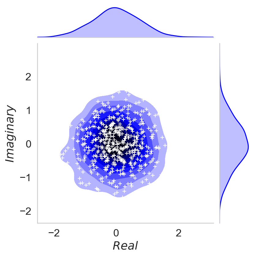 Figure 1
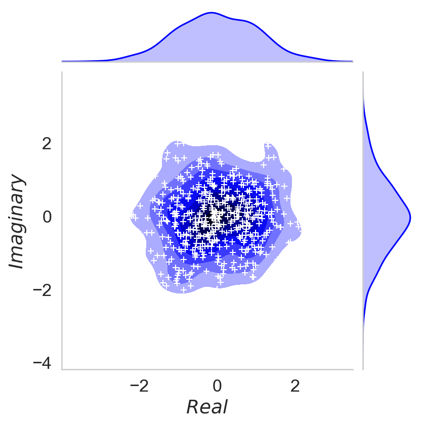 Figure 2
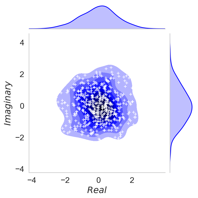 Figure 3
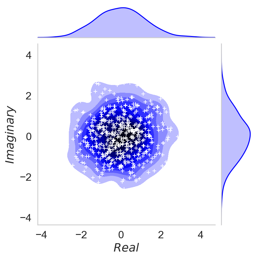 Figure 4
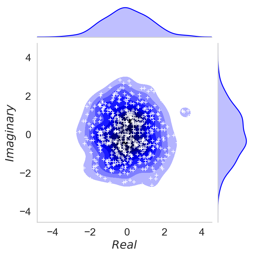 Figure 5
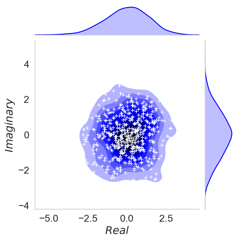 Figure 6
Peer Reviews
No public reviews on file for this paper yet. If you reviewed it on a platform where reviews are public (OpenReview, ICLR, NeurIPS, ICML), you can paste yours below so the community can read it here.
Videos
No videos yet. Explain this paper in a talk, walkthrough, or lecture? Add one.
Taxonomy
TopicsRandom Matrices and Applications · Algebraic structures and combinatorial models · Molecular spectroscopy and chirality
CLT for non-Hermitian random band matrices with variance profiles
Indrajit Jana
School of Basic Sciences, IIT Bhubaneswar, India, 752050
Abstract.
We show that the fluctuations of the linear eigenvalue statistics of a non-Hermitian random band matrix of increasing bandwidth with a continuous variance profile converges to a , where and is the test function. When , we obtain an explicit formula for , which depends on , and variance profile . When , the formula is consistent with Rider and Silverstein (2006) [33]. We also independently compute an explicit formula for i.e., when the bandwidth grows slower compared to . In addition, we show that as .
**Keywords: ** Random band matrices, random matrices with a variance profile, central limit theorem, linear eigenvalue statistics.
1. Introduction
In this article, we consider the linear eigenvalue statistics of random non-Hermitian band matrices with a variance profile. Let be an random non-Hermitian matrix and be its eigenvalues. Define the empirical spectral measure (ESM) of as
[TABLE]
where is unit point mass at . It was shown, in a series of papers, that if the entries of are i.i.d. random variables with zero mean and unit variance, then asymptotically converges to the uniform density on the unit disc in [19, 5, 16, 38, 39]. However, if the entries are not identically distributed, the limiting law may be different. In particular, when the entries of the matrix are multiplied by some predetermined weights, the matrix is called a random matrix with a variance profile. Limiting ESM of such matrices were found in [13].
In an analogous way to classical probability, limiting ESM is the law of large numbers for random matrices. One might be interested in finding fluctuations of such convergence after proper scaling, which is the central limit theorem (CLT) in classical probability. In the case of random matrices, we would be studying CLT of the sequence of random measures (the ESMs). One way to study such object is by studying for some test function . This brings the question from the space of random measures to the space of real/complex valued random variables. More precisely, we define the linear eigenvalue statistics of with respect to a test function as
[TABLE]
We consider the limiting distribution of . Limiting behavior of such quantities were studied in [22, 37, 27], [11, section 5] for Hermitian matrices; and in [4, 26, 21, 35] for Hermitian band matrices.
In this article, we consider non-Hermitian matrices whose entries are complex valued random variables. Distributional limit of such objects was found in [30, 7, 32, 33, 34], which was later extended in [2, 31, 8, 25]. CLT for polynomial and real valued were studied in [30]. More recently, CLT for products of random matrices were established in [14, 20]; and words of random matrices were studied in [15].
In both the cases [33, 30], the matrix was a full matrix without any variance profile. Recently, for polynomial test functions, it was shown that for random symmetric/non-symmetric matrices with a variance profile converges to in total variation norm [1]. However, since the results in [1] were stated in a very broad context, the exact expression of was difficult to find.
The main contribution of this article is calculating for random band matrices with a variance profile. In [33], the variance was calculated in the process of proving the CLT. The same procedure does not yield the variance in our case. So, the proof of CLT and calculation of variance is done using two separate methods. An non-periodic (and periodic) band matrix of bandwidth is obtained by keeping many off-diagonal vectors around the main diagonal (and around the corners), and setting rest of the off-diagonal vectors to zero.
A precise definition of random band matrix is given in the Definition 2.1. In particular, we show that if we have a periodic band matrix with , then our results are consistent with that of [33]. In this context, we would also like to mention that while in full matrix case the unscaled converges to a Gaussian distribution, in band case we need to scale it by . This shows a significant difference in between full and band matrices. In the first case remains constant, while in the latter case it grows as .
The article is organized as follows. In Section 2, we enlist the notations and definitions. The main theorem is formulated in Section 3, and the proof is given in Section 4. In the process of the proof, we need the norm of the random matrix to be bounded almost surely, which is discussed in appendix A. Variance of the limiting distribution is calculated in Section 5.
Acknowledgment: The author gratefully acknowledges many technical discussions with Brian Rider. The author also conveys thanks to Alexander Soshnikov; and Kartick Adhikari, Koushik Saha for mathematical discussions and sponsoring a visit to UC Davis; and providing constructive feedbacks about the manuscript. In addition, the author appreciates many constructive feedback provided by the referees.
2. Preliminaries and notations
For convenience, we do not indicate the size of a matrix in its name. For example, to denote an matrix , we simply write instead of . In addition, throughout this paper we use the following notations;
[TABLE]
Definition 2.1** (Band matrix with a variance profile).**
Let , and be a piece-wise continuous function supported on such that it is continuous at [math] and . Define a periodic function and a non-periodic function as follows
[TABLE]
In particular, on any compact subset of . Let be a set of i.i.d. random variables for each , and .
- (1)
When , define a periodic band matrix of bandwidth as
[TABLE] 2. (2)
When , define non-periodic band matrix of bandwidth as
[TABLE]
and a periodic band matrix of bandwidth as
[TABLE]
In this context, let us also define the band index set , and the band diagonal matrix as follows
[TABLE]
In particular, we observe that if and for all , then
[TABLE]
where is the th column of , which is one of the in the above.
In the above definition, we notice that if we take , then it yields band matrices without any variance profile i.e., identical variances. We also observe that if the periodic band matrix is a full matrix then .
We would also like to mention that when , we are considering only periodic band matrices; and when , we are considering both periodic and non-periodic band matrices. In short, we are not considering non-periodic band matrices when . The CLT may still be true for non-periodic band matrices with . However, our method of variance calculation does not work in this case; as outlined in Remarks 5.1, 5.2.
Definition 2.2** (Poincaré inequality).**
A complex random variable is said to satisfy Poincaré inequality with constant if for any differentiable function , we have . Here is identified with .
Here are some properties of Poincaré inequality
- (1)
If satisfies Poincaré inequality with constant , then also satisfies Poincaré inequality with constant for any . 2. (2)
If two independent random variables satisfy the Poincaré inequality with the same constant , then for any differentiable function , i.e., also satisfies Poincaré inequality with the same constant . 3. (3)
[3, Lemma 4.4.3] If satisfies Poincaré inequality with constant , then for any differentiable function
[TABLE]
where . Here is identified with . In the above, denotes the norm of the -dimensional vector at ; and . In particular if is a Lipschitz function with lipschitz constant , then .
For example, Gaussian random variables and compactly supported continuous random variables satisfy Poincaré inequality.
3. Main result
Condition 3.1**.**
Let be an i.i.d. set of complex-valued continuous random variables, and be one of the random band matrices as defined in the Definition 2.1. Assume that
- (i)
and for all , 2. (ii)
s are continuous random variables with bounded density and satisfy the Poincaré inequality with some universal constant . In particular, for all and for some universal constant . 3. (iii)
Either of the following is true.
- (a)
, and for all ; , 2. (b)
and for all .
Here the Poincaré inequality is assumed for both as well as to unify the proof. However in the latter case i.e., , the proof may go through using the techniques of [33] without Poincaré inequality. Also in (iii)(a), it suffices to take (see (4.19)) for some . But we assume for simplicity.
The above conditions implies that for some fixed almost surely as . We shall discuss this in more details in appendix A.
Theorem 3.2**.**
Let be one of the random band matrices of bandwidth as defined in the Definition 2.1 such that condition 3.1 holds. Let be analytic on for some and bounded elsewhere.
Then as ,
[TABLE]
where ,
[TABLE]
and
[TABLE]
Here
[TABLE]
We give the proof in Section 4 and variance is calculated in Section 5. Before going into the proof, we would like to make some remarks about the above theorem. First of all, the theorem is stated for ; not for . To the best of our knowledge, the circular law for random band matrices is not known for . If the circular law is true for random band matrices, we would asymptotically have
[TABLE]
Then asymptotically we would have .
Secondly, if is a non-Hermitian full matrix with a continuous variance profile , then . Limiting ESM of such matrices was discovered in [12]. The following corollary provides a CLT for such matrices.
Corollary 3.3**.**
Let be a non-Hermitian random matrix with a variance profile as defined in Definition 2.1 such that condition 3.1 holds. Let be analytic on for some and bounded elsewhere.
Then as ,
where ,
[TABLE]
[TABLE]
It should be noted that we can also have without having a full matrix; for example, by replacing many off diagonals of a full matrix by zeros. The above corollary along with Theorem 3.2 asserts that the limiting Gaussian distribution will be unchanged by doing so. In addition to the above corollary, we discuss a few more particular cases.
- (I)
If we have the full matrix with i.i.d. entries, then , and . In that case, . As a result,
[TABLE]
The above is the same as the expression obtained in [33]. In particular, if , then for all . A numerical evidence of this fact is outlined in table 1. 2. (II)
Let and be a periodic band matrix as defined in Definition 2.1 with variance profile . Consider the monomial test function . Then as a consequence of Theorem 3.2, we have , where
[TABLE]
and . The above equality follows from the fact that
[TABLE] 3. (III)
Let and , then where
[TABLE]
The above follows from the second part of the Theorem 3.2 and the fact that
[TABLE]
The last equality of (3.1) was obtained by establishing a connection to Irwin-Hall distribution which is outlined in Section 5.4. In addition if is even, one can also write
[TABLE]
where is an Eulerian number. In combinatorics, counts the number of permutations of the numbers in which exactly elements are greater then the previous element. 4. (IV)
We have the following table regarding integrals of the function [29].
[TABLE]
From the above equations, we obtain
[TABLE]
Figure 3 shows some simulations done in Python. We have taken periodic random band matrix with i.i.d. complex variables. We run the simulation for test functions and varying bandwidth.
4. Proof of the Theorem 3.2
We adopt the methods based on [33, 35]. Let us define the event
[TABLE]
where is the same as in Lemma A.3. From Lemma A.3 we also have that
[TABLE]
So, if is analytic on , then on the event we may write
[TABLE]
where . While the above is true for any such function , the readers may think of as a linear combination of from theorem 3.2. Let us define
[TABLE]
Now we decompose as
[TABLE]
In the due course, we would like to show that
[TABLE]
and converges to an appropriate Gaussian process.
Proof of 4.2.
First of all since the entries of are continuous random variables, . Which implies that . Therefore
[TABLE]
∎
Proof of 4.3.
To prove (4.3), we expand on for as follows
[TABLE]
On , the last term is bounded by for all .
Now from the condition 3.1(ii, iii) and boundedness of , we shall show that for any
[TABLE]
where is a universal constant.
Under 3.1(iii)(a), it follows that . Otherwise under condition 3.1(iii)(b), . Therefore non-trivial contributions in (in terms of ) are obtained when each random variable appears at least three times. There are at most different ways to partition in which each partition size at least three. In each case, , and the expectation is bounded by (by condition 3.1(ii)). On the other hand, due to normalization by , the denominator is . Combining the two, we have the result (4.5).
Using the equation (A.3) along with Hölder’s inequality, we have
[TABLE]
for and large enough . Here is a universal constant.
In addition, . As a result taking expectation in (4.4) after multiplying by , and using (4.6), (4.5) we have
[TABLE]
where for all , the constant depends uniformly on and . This completes the proof of (4.3).
∎
Therefore, asymptotically we may write
[TABLE]
Thus, proving the Theorem 3.2 is equivalent to proving the following proposition.
Proposition 4.1**.**
The sequence is tight in the space of continuous functions on , and converges in distribution to a Gaussian process with covariance kernel
[TABLE]
Remark 4.2**.**
Note that since is continuous and , we have for all , . Here stands for the Fourier transform of . Therefore is well defined for and analytic on for any . On the other hand, s are analytic. Therefore the value of is same for any . This justifies the integrals in the Theorem 3.2 are over instead of .
Now, we move to the proof of Proposition 4.1. By Cramér-Wold device, it suffices to show that for any and for which
[TABLE]
is real; converges to a Gaussian random variable with mean zero and variance . In this Section, we shall show that it converges to a Gaussian process with mean zero and unknown variance. The exact computation of variance is done in Section 5.
We use the martingale difference technique from Lemma B.1 to establish the above. Let be the averaging with respect to the th column of , and . Clearly, and . We write as
[TABLE]
where . Clearly, is a martingale difference sequence with respect to the filtration . Rewrite (4.14) as
[TABLE]
Clearly, is a martingale difference sequence with respect to the filtration . Notice that . Therefore, condition of Lemma B.1 is equivalent to
[TABLE]
And the condition of Lemma B.1 is equivalent to
[TABLE]
Thus proving the Proposition 4.1 is equivalent to showing the tightness of and (4), (4.17), (4.18). We do the following general reductions before the proof.
Let be obtained by setting the th column of to zero, and , where . The resolvent identity yields . We show that replacing by in (4.15) is asymptotically same in probability.
[TABLE]
Therefore using resolvent identity and Lemma B.2, we have
[TABLE]
where
[TABLE]
We notice that is a product of two independent random variables. Intuitively, conditioned on , almost surely. We give the exact estimate below.
Define . Then using the property 3 in Definition 2.2 and the fact that for , we have
[TABLE]
where . The factor is obtained by using Definition 2.2(1) and the fact that each entry of is scaled by the variance profile and . Now, taking and using the fact that we have . Hence by Borel–Cantelli lemma, we have . In addition, we also get that
[TABLE]
We notice that
[TABLE]
Because is independent of the th column . Consequently,
[TABLE]
Now we show that the above expectation exists. Let be the pdf of . Since the pdf of each are bounded (condition 3.1(ii)), by Young’s convolution inequality, . So for any and large enough ,
[TABLE]
where is a universal constant. Taking further expectation,
[TABLE]
Similarly also using (4.19), . Therefore, we have
[TABLE]
where the switching between and can be justified by the dominated convergence theorem and (4.21). The above technique rewrites in terms of derivative of an analytic function, which will allow us to estimate via the following basic fact from complex analysis;
[TABLE]
where is analytic on .
4.1. Proof of tightness
This part is similar to Section 3.2 in [33]. In this subsection, we show that is tight in , the space of continuous functions on . In other words, for any there exists a compact set such that
[TABLE]
However, the compact sets in the space of continuous functions are the space of equicontinuous functions.
Let us define,
[TABLE]
By (4.19), and simple union bound
[TABLE]
The last equality follows from the assumption that . Consequently,
[TABLE]
for any . Now, (4.24) follows from Markov’s inequality and the following condition;
[TABLE]
uniformly for all and . In what follows, the methods are similar to [33]. For the sake of completeness, we outline it here.
Using the resolvent identity, we can write
[TABLE]
Thus, in the view of (4.15)
[TABLE]
Using resolvent identity and Lemma B.2,
[TABLE]
In the view of (4.20), we have . Therefore we can rewrite (4.26) as
[TABLE]
Since is a martingale difference sequence,
[TABLE]
Therefore, proving (4.25) is equivalent to showing that
[TABLE]
uniformly for all and . However, applying the same method as described in (4.19), we can get similar tail estimates for etc. (with or in the rhs of (4.19)). Now since on , using the estimate in s, we have (4.27).
4.2. Proof of (4)
Expanding up to two terms and using (4.19), (4.22), (4.23) we have
[TABLE]
Substituting the above in (4), we obtain
[TABLE]
which proves the result.
4.3. Proof of (4.17)
Using condition 3.1(iii), (4.19) and expanding up to two terms, we see that
[TABLE]
Thus, using (4.22), (4.23) and the above we have
[TABLE]
which proves (4.17).
4.4. Proof of (4.18)
Expanding up to two terms and using (4.19), (4.22) we have
[TABLE]
where
[TABLE]
As a result, (4.18) becomes
[TABLE]
Now since on , is a sequence of uniformly bounded analytic functions on . Therefore by Vitali’s theorem (eg. [40, Theorem 5.21]), proving (4.18) equivalent to show that converges in probability.
Since is a martingale difference sequence, we have if . As a result,
[TABLE]
Limit of the above is calculated in Section 5. Here we show that .
Recall
[TABLE]
Let , and be a smooth function such that
[TABLE]
Let us define and
[TABLE]
We note the following estimate
[TABLE]
Using the Lemma A.3, we have
[TABLE]
For notational simplicity, let us denote
[TABLE]
where denotes the diagonal matrix by taking square root of each entry of the diagonal matrix . Then . Since s satisfy Poincaré inequality, we have
[TABLE]
The first sum stops at because is constant as a function of columns of . On the other hand, we have
[TABLE]
Consequently,
[TABLE]
Denoting and using the facts that , we have
[TABLE]
Using the above estimates, (4.1), and the fact that we have,
[TABLE]
No using the estimate (4.28) and the assumption , we conclude that
[TABLE]
5. Calculation of the variance
Let us first find the variance for monomial test functions. Let us define .
5.1. Case I:
The matrix in Definition 2.1 is periodic.
[TABLE]
In the above expression, the maximum contribution (in terms of ) occurs when all the indices in the loop are distinct and the loop overlaps with the loop . The reasoning is similar to (4.5). Once the indices are fixed, the loop must be same as the loop . However, they can overlap in different ways by rotating .
Now the first index can be chosen in different ways. After that, while choosing the remaining many indices, due to the band matrix structure, each index has to be within neighborhood of the previous index such that the final index is also within neighborhood of the first index as well.
This last condition imposes an additional constraint which is not present in the full matrix cases. However, these band constraints are completely handled by the weight profile . Therefore using the structures of s from Definition 2.1, we have
[TABLE]
where denotes the fold convolution, and
[TABLE]
is the th Fourier coefficient of . Note that in any fold convolution, the integral is taken over many variables only (as in 5.1). In our context, this can also be explained by the fact that for each chosen index , we have freedom to choose the indices only.
Remark 5.1**.**
The integral (5.1) is taken over , because for all . However, the values of the variables may fall outside in principle. But using the periodicity of , we can bring it back to . The above calculation does not work for non-periodic band matrices while .
5.2. Case II:
The band matrix in Definition 2.1 is periodic. In that case, we compute
[TABLE]
where
[TABLE]
Remark 5.2**.**
In the above, if the band matrix was not periodic, we can make the above integration over i.e., fold convolution, by taking far off from the origin. We can do that because of . Thus, the above calculation will also go through for non-periodic band matrices. However, the same approach can not be implemented in (5.1), as in that case . So, we need the matrix to be periodic when .
5.3. Covariance kernel of
In the view of (4.5), we notice that if then
[TABLE]
If , then
[TABLE]
Therefore using (5.2), Lemma A.3 for , and proceeding as (4.4), (4.6) on page 4.4 we have,
[TABLE]
where the last expression follows from the fact that . If we take in the above expression, we obtain
[TABLE]
Alternatively when , using (5.5),
[TABLE]
5.4. Connection to Irwin-Hall distribution & Eulerian numbers
Suppose the weight profile . Then (5.4) can be written as , where
[TABLE]
and . Let and be the pdf of . Since follows the Irwin-Hall distribution, the density of is given by
[TABLE]
For a geometric derivation of the above formula, see [28]. On the other hand, the characteristic function of is given by
[TABLE]
Using the inversion formula,
[TABLE]
Therefore,
[TABLE]
where is an Eulerian number for even . counts the number of permutations of in which exactly elements are bigger than the previous element. The above establishes (3.1).
Appendix A
In this section we discuss about norm of random non-Hermitian matrices. A sharp almost sure bound on the spectral radius of non-Hermitian random matrices can be found in [17, 18].
Theorem A.1**.**
[18]** Let be a sequence of random matrices with real valued i.i.d. for each . Assume that for each ,
- (i)
** 2. (ii)
** 3. (iii)
* for all and for some .*
Let
[TABLE]
Then almost surely.
We see that in our context if a full random matrix satisfies the condition 3.1, then it also satisfies the above condition and as a result, almost surely as . However, the above theorem does not take a variance profile into account. The following theorem from [6] estimates the norm of a symmetric random matrix with a variance profile.
Theorem A.2**.**
[6, Corollary 3.5]** Let be a real symmetric matrix with , where are independent centered random variables and are give scalars. If for some and all , then
[TABLE]
where depends on only.
Using the above theorem along with Poincaré inequality, we have the following lemma.
Lemma A.3**.**
Let be an random matrix as in the Theorem 3.2. Then there exists such that
[TABLE]
where is a universal constant. In particular,
[TABLE]
Proof.
First of all, we may write , where both and are real valued matrices. Then we can estimate . Therefore without loss of generality, let us consider be a real valued matrix. Consider
[TABLE]
and apply theorem A.2 on to obtain the same bound for . In our case, or as described in Definition 2.1. Since and is a piece-wise continuous function, and . As a result, there exists such that
[TABLE]
Here we note that we need to grow at least as . In fact, this is a sharp condition. Otherwise, the matrix norm may be unbounded [10, 23].
Secondly, implies that is a Lipschitz1 function. Therefore applying the properties of Poincaré inequality as described in Definition 2.2, we have
[TABLE]
where .
Equation (A.2) can be seen from the equation (A.1) along with the application of Borel-Cantelli lemma with . Equation (A.3) can be justified as follows,
[TABLE]
We would like to remark that the lemma is also true for column removed matrices , and the same proof will go through. ∎
We finally would like to remark that although the Theorem A.2 gives a constant bound on the norm of the matrix with a variance profile, the constant is not that sharp unlike Theorem A.1. However, we expect that for matrices with continuous variance profile, the correct norm bound should be . This was remarked in [24, Remark 4.11]. In our case, this limit is equal to . As we have mentioned in remark 4.2 that eventually it suffices to take only.
Appendix B
Here we list down the two key ingredients; martingale difference CLT, and Sherman-Morrison formula. Interested readers may find the proofs in the included references.
Lemma B.1**.**
[9, Theorem 35.12]** Let be a martingale difference array with respect to a filtration . Suppose for any ,
- (i)
, 2. (ii)
* as .*
Then .
Lemma B.2** ([36], Sherman-Morrison formula).**
Let and be two invertible matrices, where . Then
[TABLE]
The reference list from the paper itself. Each links out to its DOI / PubMed record.
- 1[1] K. Adhikari, I. Jana, and K. Saha. Linear eigenvalue statistics of random matrices with a variance profile. ar Xiv preprint ar Xiv:1901.09404 , 2019.
- 2[2] Y. Ameur, H. Hedenmalm, and N. Makarov. Fluctuations of eigenvalues of random normal matrices. Duke mathematical journal , 159(1):31–81, 2011.
- 3[3] G. W. Anderson, A. Guionnet, and O. Zeitouni. An introduction to random matrices . Number 118. Cambridge University Press, 2010.
- 4[4] G. W. Anderson and O. Zeitouni. A CLT for a band matrix model. Probab. Theory Related Fields , 134(2):283–338, 2006.
- 5[5] Z. Bai et al. Circular law. The Annals of Probability , 25(1):494–529, 1997.
- 6[6] A. S. Bandeira and R. Van Handel. Sharp nonasymptotic bounds on the norm of random matrices with independent entries. The Annals of Probability , 44(4):2479–2506, 2016.
- 7[7] R. Bauerschmidt, P. Bourgade, M. Nikula, and H.-T. Yau. The two-dimensional coulomb plasma: quasi-free approximation and central limit theorem. ar Xiv preprint ar Xiv:1609.08582 , 2016.
- 8[8] F. Bekerman, T. Leblé, S. Serfaty, et al. Clt for fluctuations of β 𝛽 \beta -ensembles with general potential. Electronic Journal of Probability , 23, 2018.