Non-equilibrium three-dimensional boundary layers at moderate Reynolds numbers
Adri\'an Lozano-Dur\'an, Marco Giometto, George I. Park, Parviz Moin

TL;DR
This study investigates non-equilibrium three-dimensional boundary layers at moderate Reynolds numbers, revealing a self-similar reduction in Reynolds stress due to flow displacement and pressure-strain effects, with implications for turbulence modeling.
Contribution
It introduces a multiscale model explaining Reynolds stress reduction in non-equilibrium 3D turbulence, validated through direct numerical simulations at Reynolds numbers up to 1,000.
Findings
Reynolds stress decreases with 3D strain and flow displacement.
Flow regimes follow a self-similar evolution pattern.
Pressure-strain correlation reduction inhibits Reynolds stress generation.
Abstract
Non-equilibrium wall turbulence with mean-flow three-dimensionality is ubiquitous in geophysical and engineering flows. Under these conditions, turbulence may experience a counter-intuitive depletion of the turbulent stresses, which has important implications for modelling and control. Yet, current turbulence theories have been established mainly for statistically two-dimensional equilibrium flows and are unable to predict the reduction in the Reynolds stress magnitude. In the present work, we propose a multiscale model which explains the response of non-equilibrium wall-bounded turbulence under the imposition of three-dimensional strain. The analysis is performed via direct numerical simulation of transient three-dimensional turbulent channels subjected to a sudden lateral pressure gradient at friction Reynolds numbers up to 1,000. We show that the flow regimes and scaling properties…
Click any figure to enlarge with its caption.
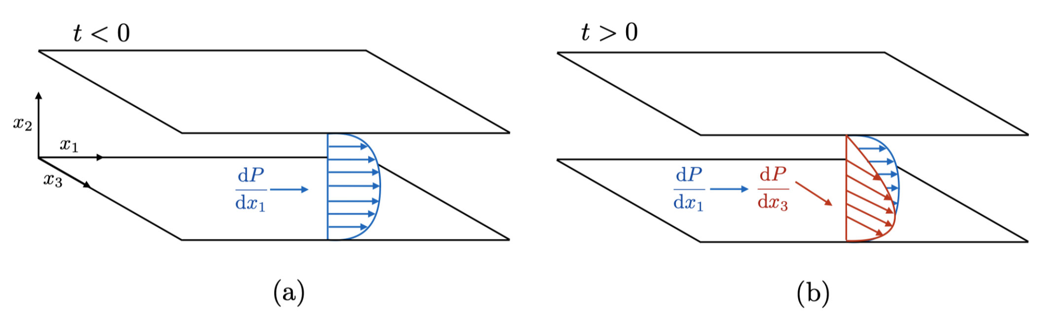 Figure 1
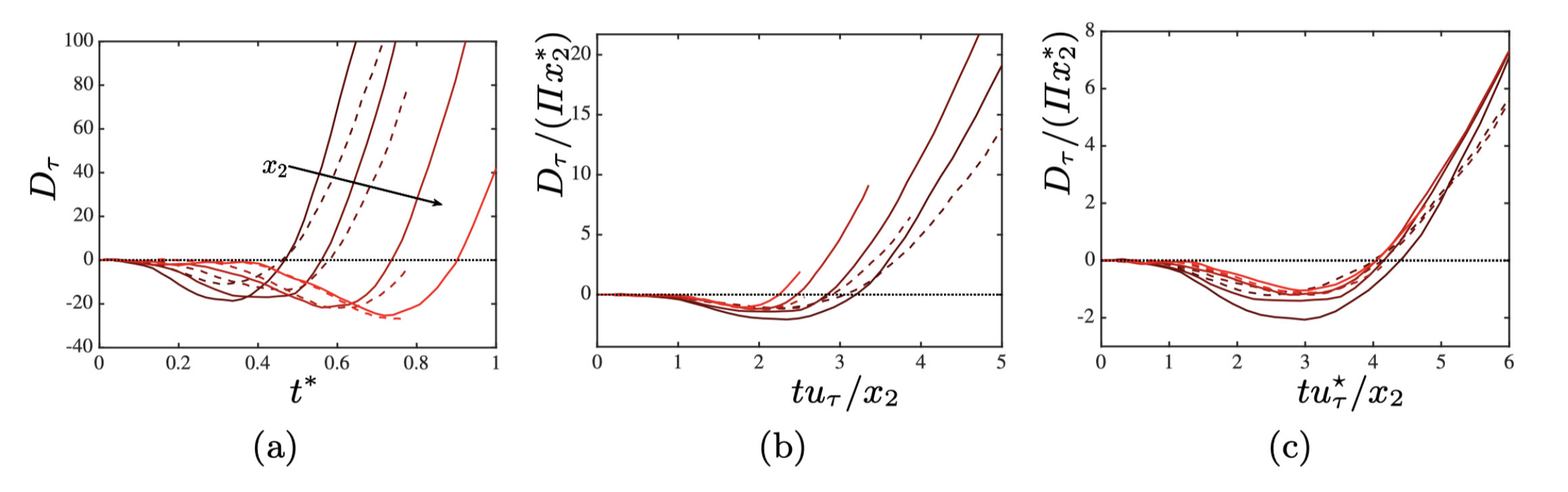 Figure 10
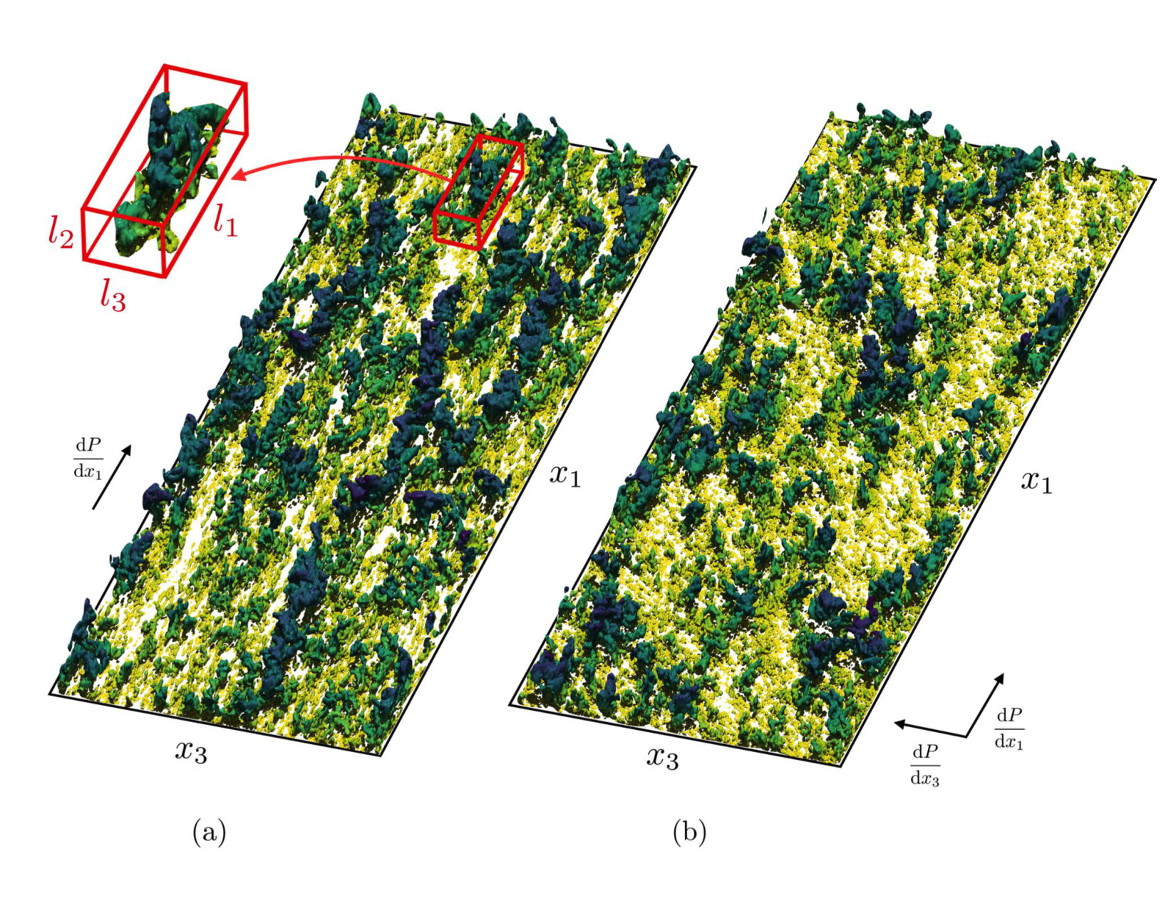 Figure 11
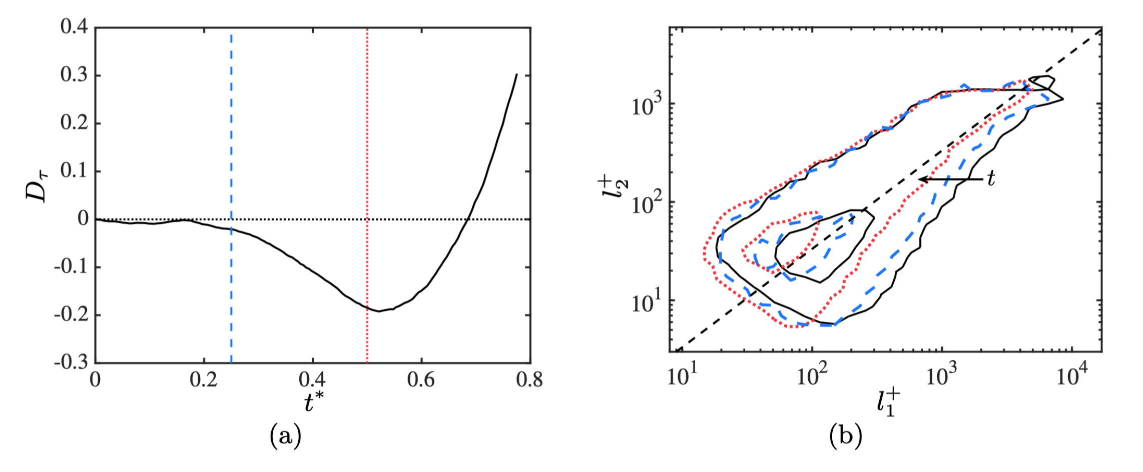 Figure 12
 Figure 13
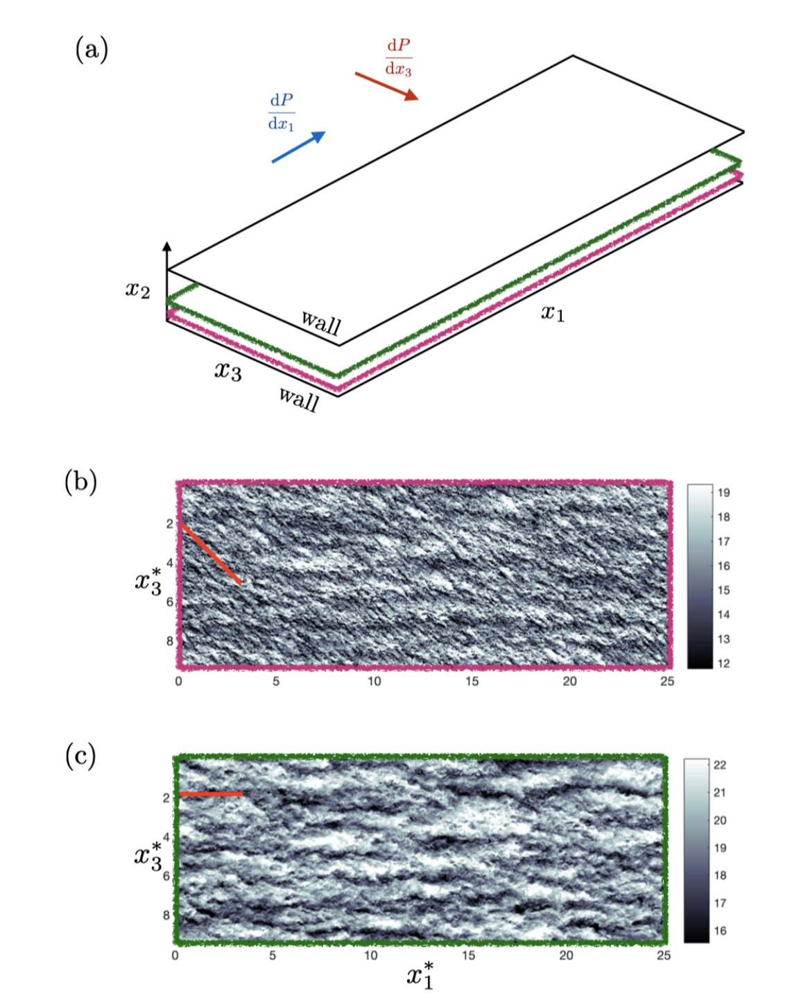 Figure 14
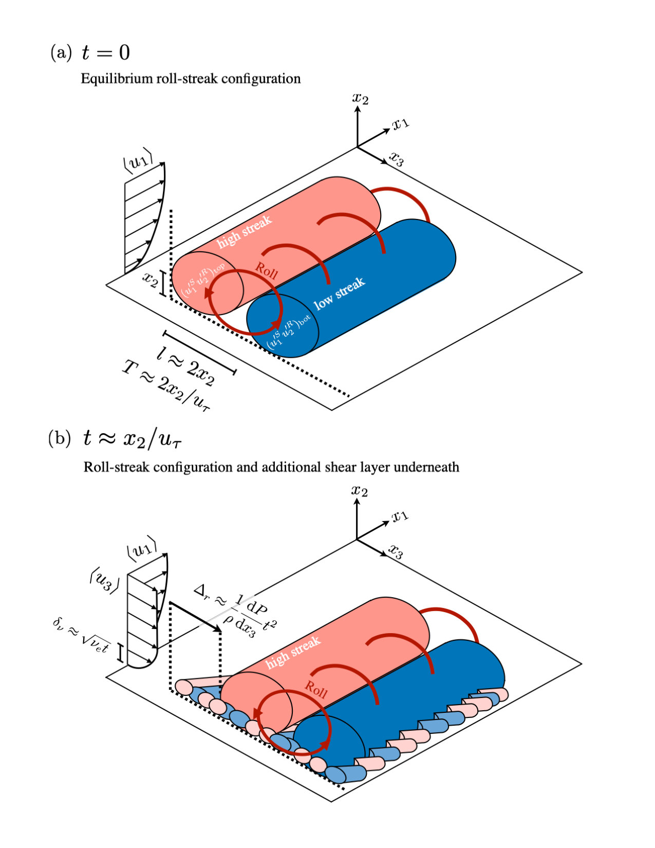 Figure 15
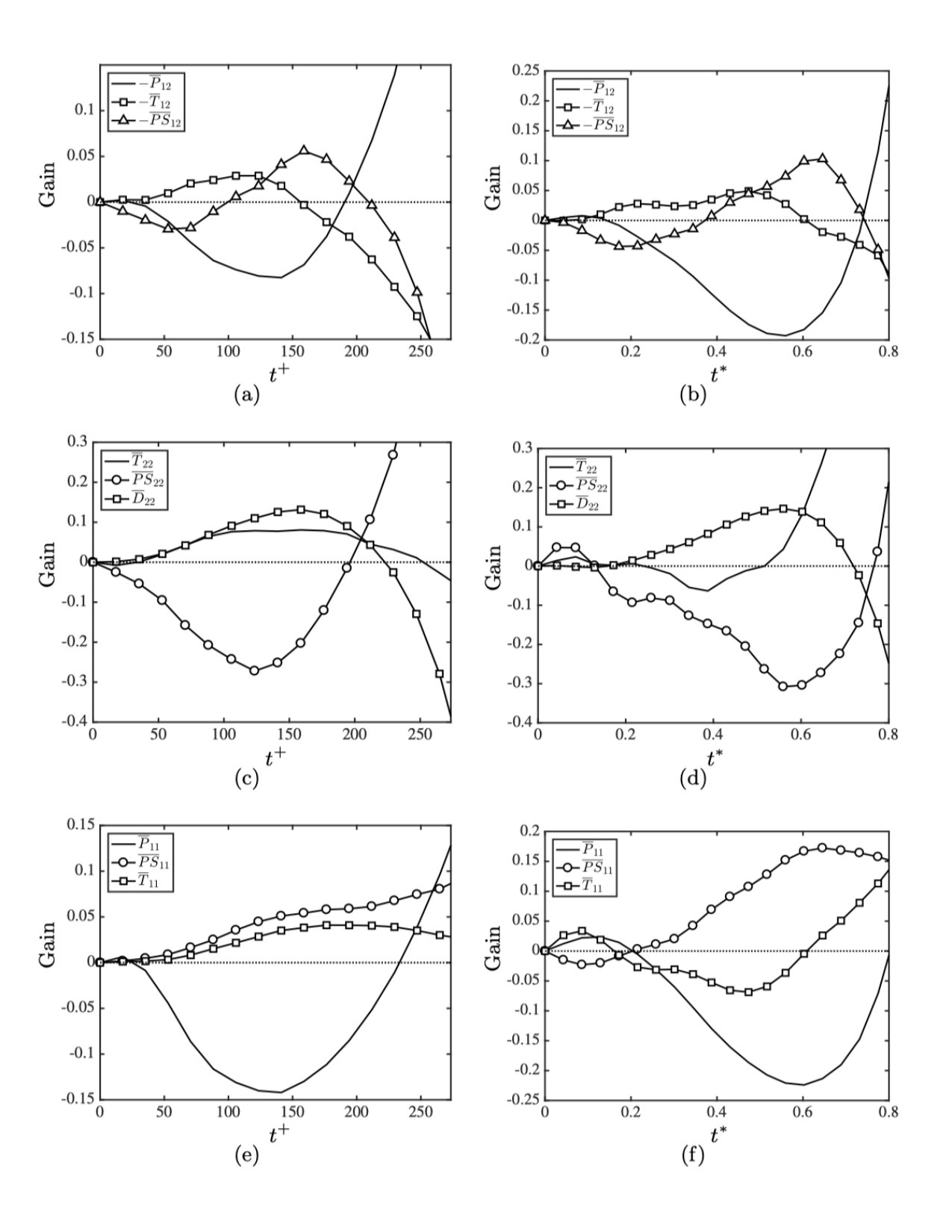 Figure 16
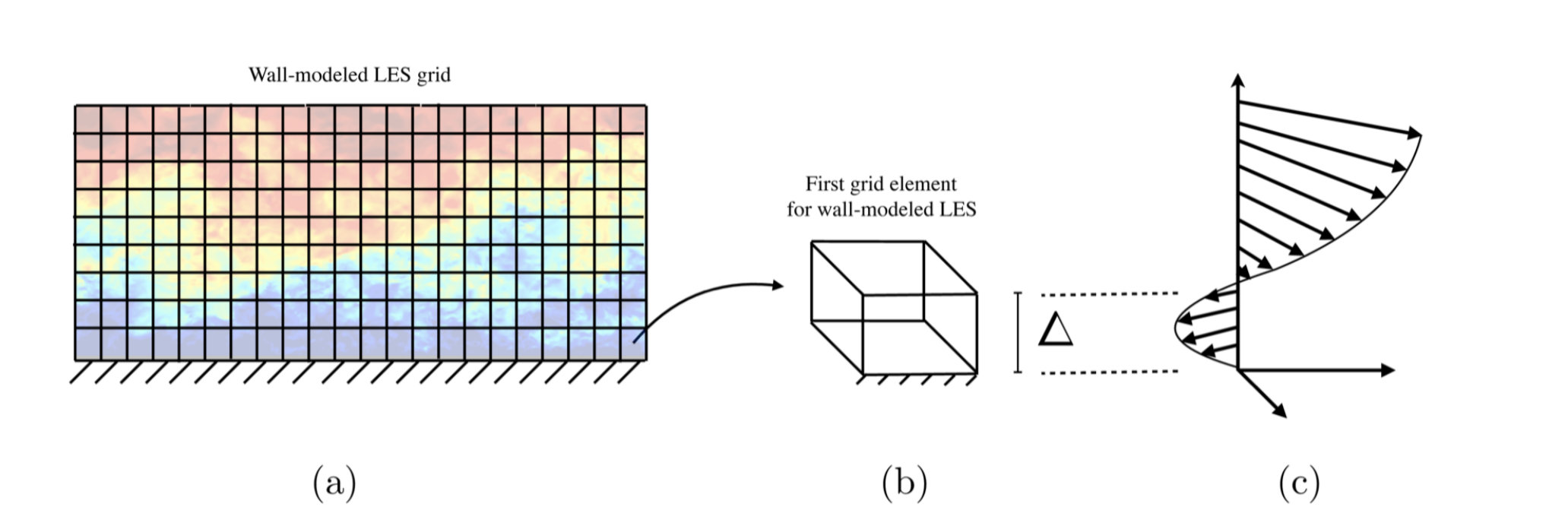 Figure 17
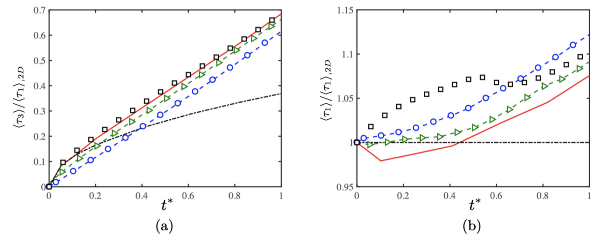 Figure 18
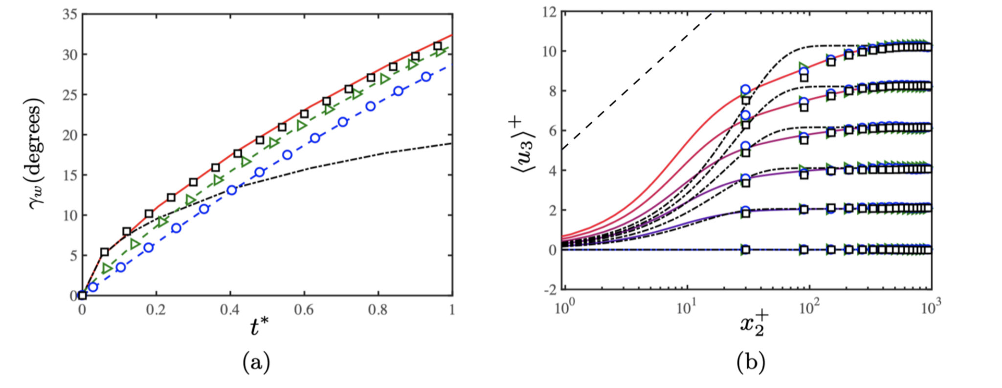 Figure 19
 Figure 2
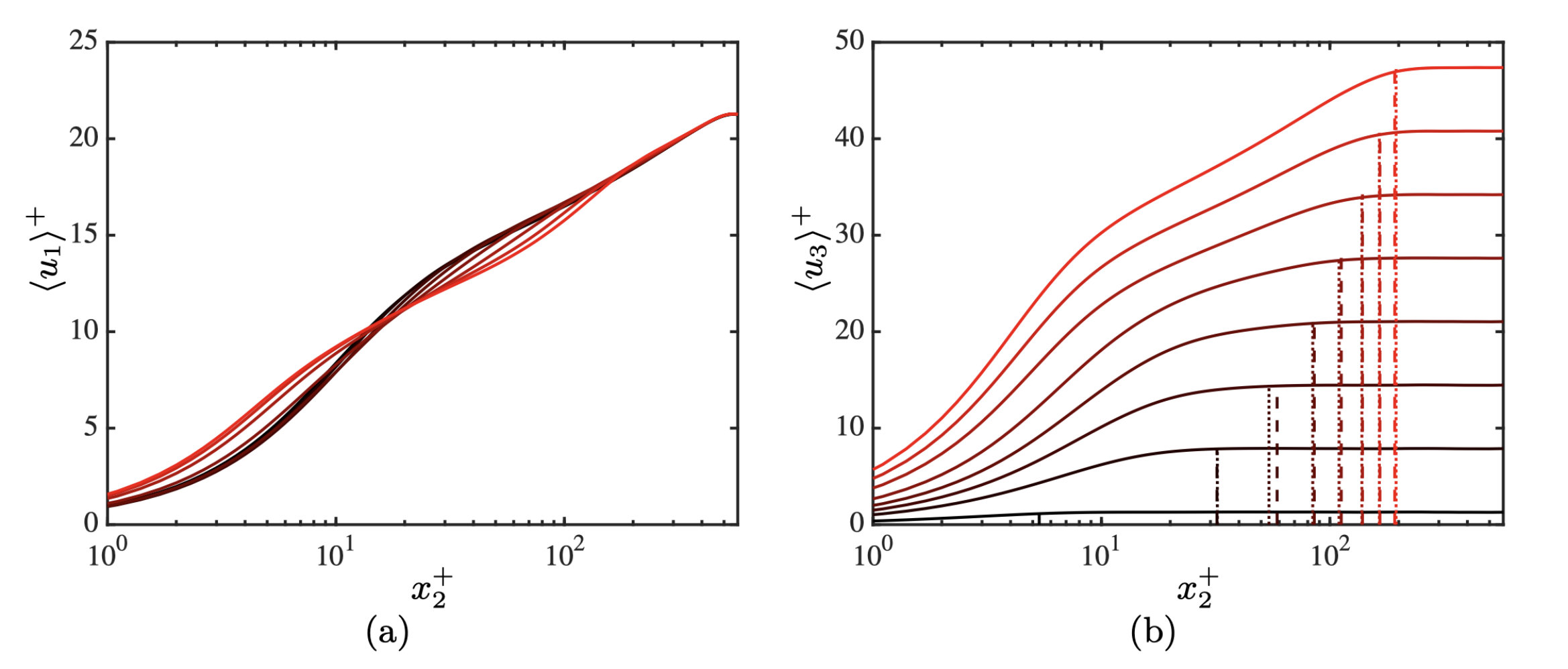 Figure 3
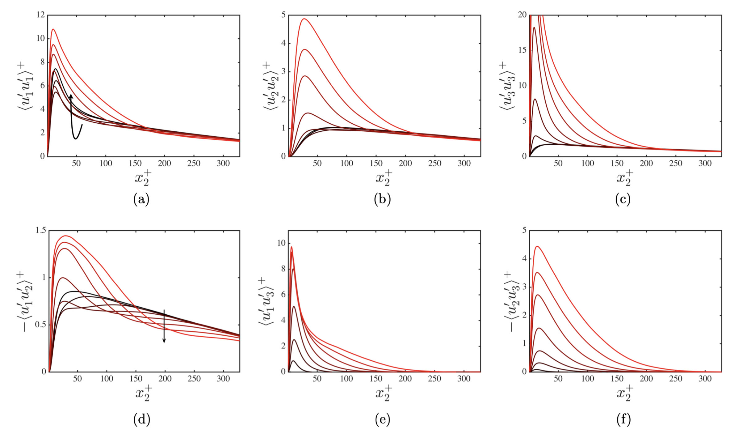 Figure 4
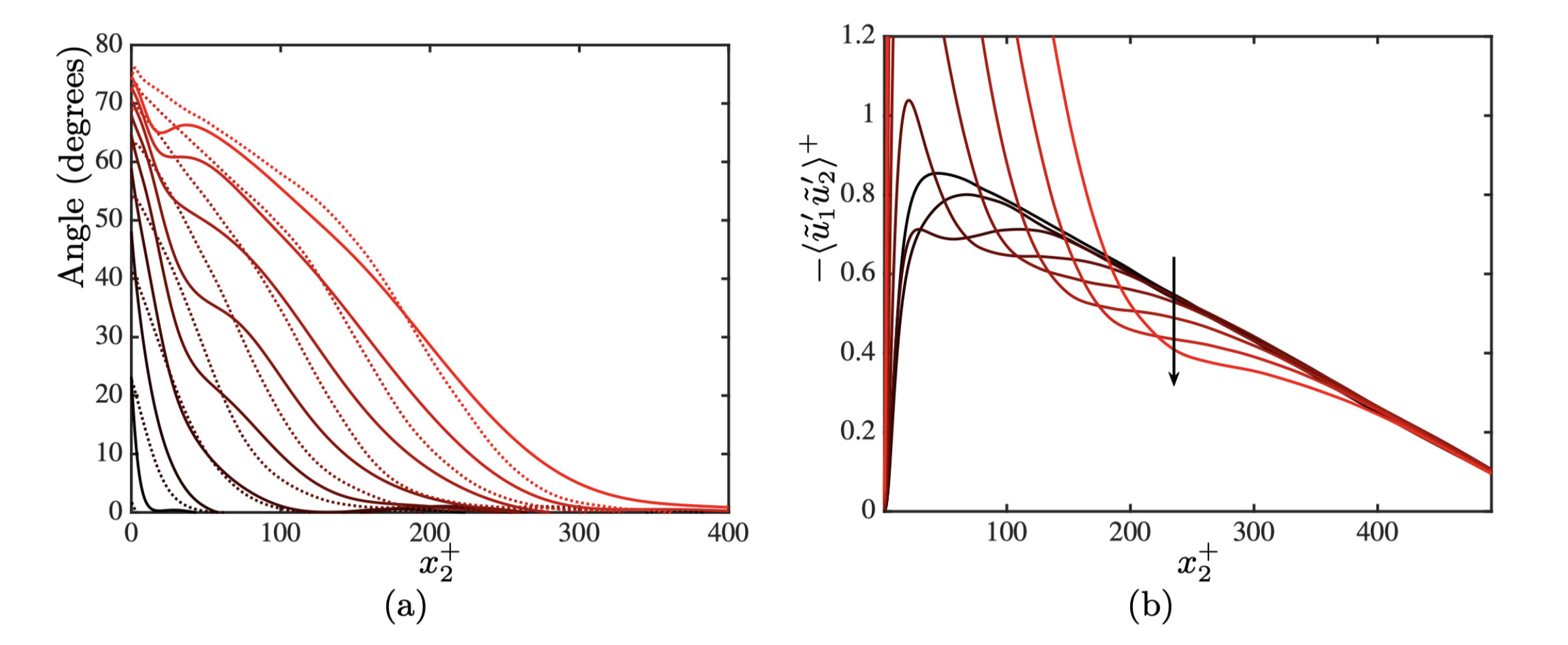 Figure 5
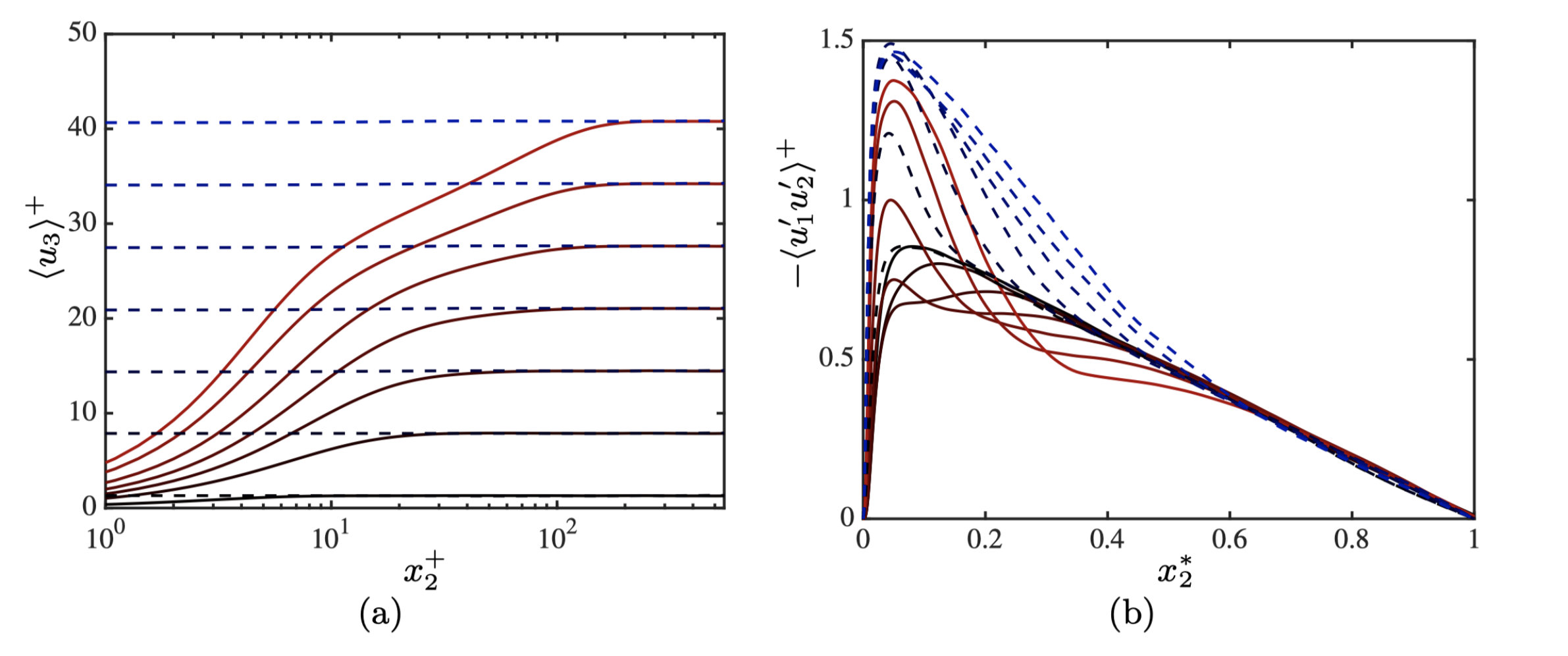 Figure 6
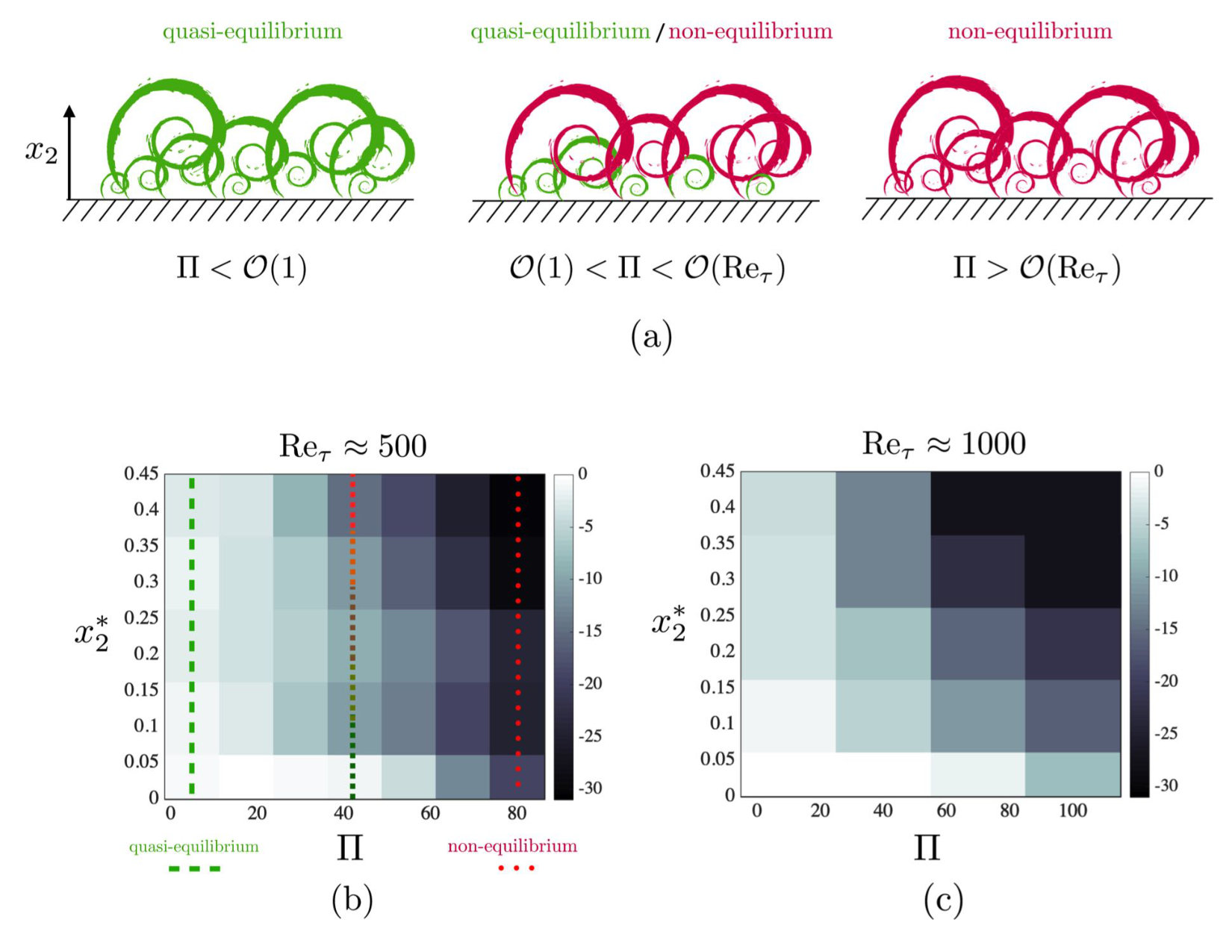 Figure 7
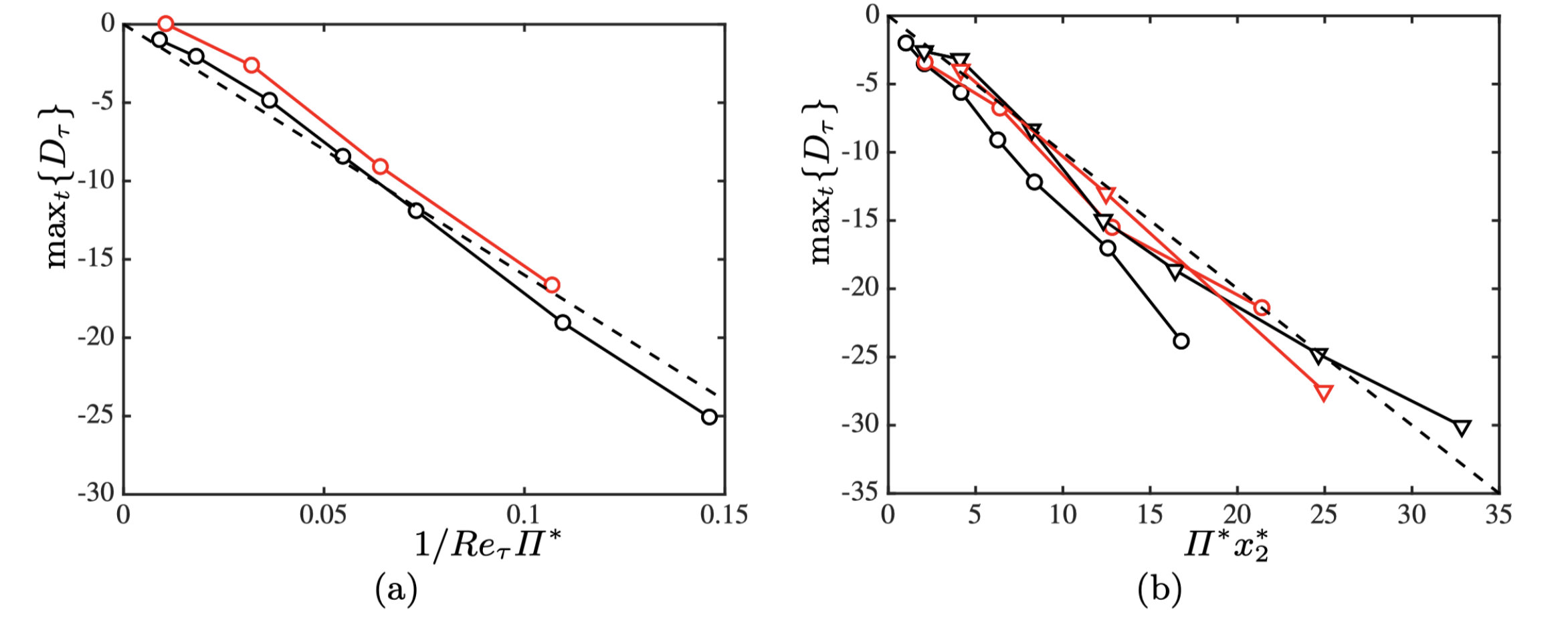 Figure 8
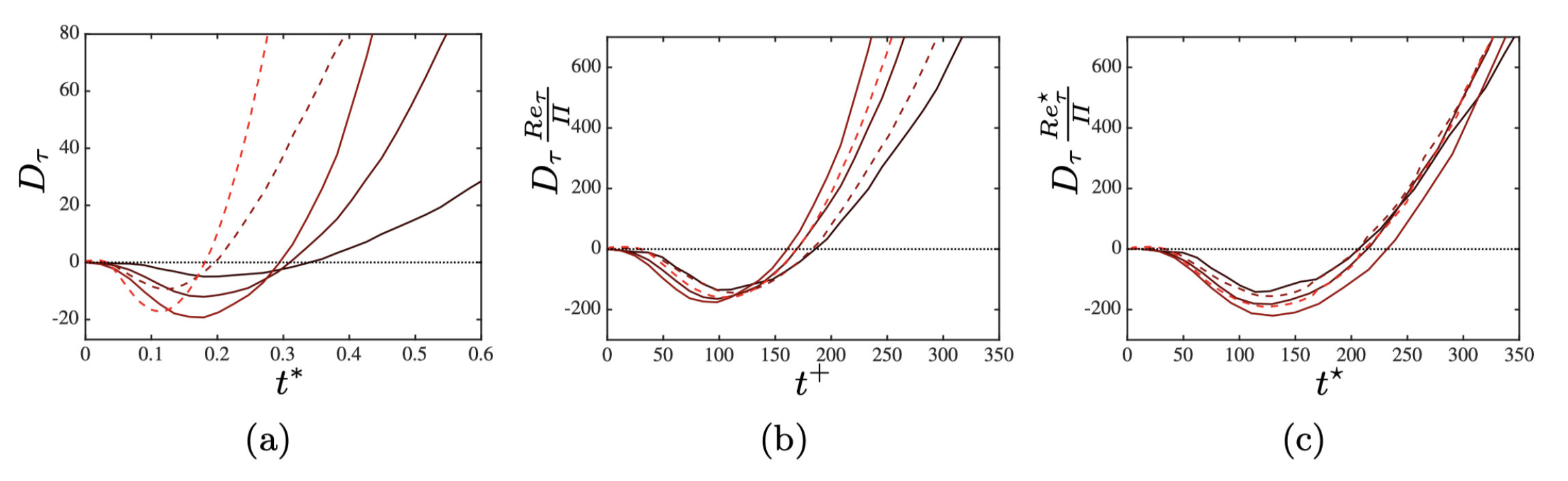 Figure 9
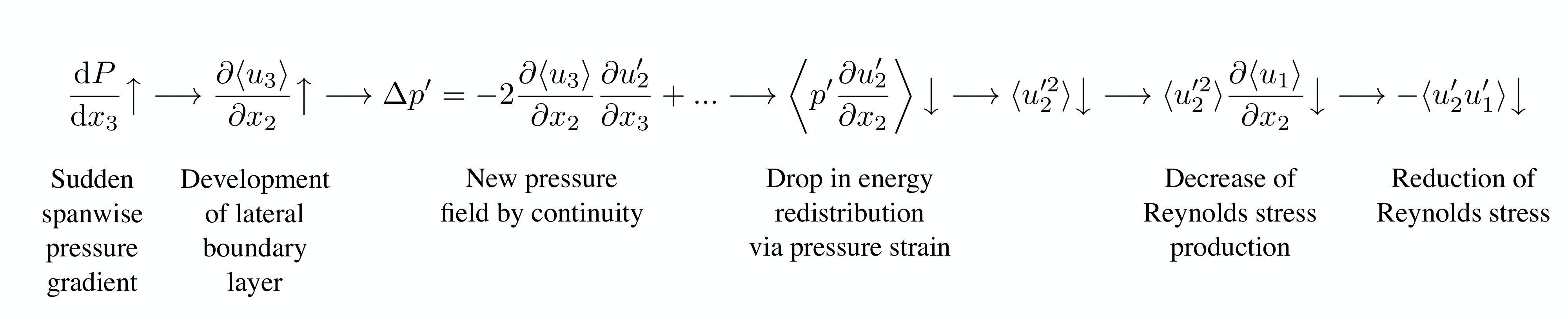 Figure 20
| 546 | 8.92 | 4.46 | 0.26 | 6.5 | 0,5,10,20,30,40,60,80 | 10 | ||||
| 934 | 7.36 | 4.29 | 0.35 | 6.7 | 0,10,30,60,100 | 5 |
Peer Reviews
No public reviews on file for this paper yet. If you reviewed it on a platform where reviews are public (OpenReview, ICLR, NeurIPS, ICML), you can paste yours below so the community can read it here.
Videos
No videos yet. Explain this paper in a talk, walkthrough, or lecture? Add one.
Non-equilibrium three-dimensional boundary layers at moderate Reynolds numbers
Adrián Lozano-Durán1\corresp
Marco Giometto2
George I. Park3
& Parviz Moin1
1Center for Turbulence Research, Stanford University, California 94305, USA
2Department of Civil Engineering and Engineering Mechanics, Columbia University, New York, 10027, USA
3Department of Mechanical Engineering and Applied Mechanics, University of Pennsylvania, Philadelphia, Pennsylvania 19104, USA
Abstract
Non-equilibrium wall turbulence with mean-flow three-dimensionality is ubiquitous in geophysical and engineering flows. Under these conditions, turbulence may experience a counter-intuitive depletion of the turbulent stresses, which has important implications for modelling and control. Yet, current turbulence theories have been established mainly for statistically two-dimensional equilibrium flows and are unable to predict the reduction in the Reynolds stress magnitude. In the present work, we propose a multiscale model which explains the response of non-equilibrium wall-bounded turbulence under the imposition of three-dimensional strain. The analysis is performed via direct numerical simulation of transient three-dimensional turbulent channels subjected to a sudden lateral pressure gradient at friction Reynolds numbers up to 1,000. We show that the flow regimes and scaling properties of the Reynolds stress are consistent with a model comprising momentum-carrying eddies with sizes and time scales proportional to their distance to the wall. We further demonstrate that the reduction in Reynolds stress follows a spatially and temporally self-similar evolution caused by the relative horizontal displacement between the core of the momentum-carrying eddies and the flow layer underneath. Inspection of the flow energetics reveals that this mechanism is associated with lower levels of pressure-strain correlation which ultimately inhibits the generation of Reynolds stress. Finally, we assess the ability of the state-of-the-art wall-modelled large-eddy simulation to predict non-equilibrium, three-dimensional flows.
keywords:
1 Introduction
Our current understanding of wall turbulence is largely rooted in studies of equilibrium boundary layers with two-dimensional (2-D) mean velocity profiles (i.e., contained in a plane). However, non-equilibrium turbulence with mean-flow three-dimensionality is the rule rather than the exception in most geophysical and engineering flows. Prominent examples of the former are Ekman layers and spirals, flow in complex terrain, tornadoes, and river bends, while industrial flows include flow over swept-wing aircrafts and hulls of marine vehicles, around buildings and obstacles, within turbomachines, etc. Despite the ubiquity of such flows, fundamental questions remain unanswered regarding the structural changes of wall turbulence under three-dimensional (3-D) non-equilibrium conditions, challenging our intellectual ability to comprehend and predict wall turbulence in broader scenarios. In the present work, we study the transition of statistically stationary 2-D turbulence to non-stationary 3-D states induced by the sudden application of a spanwise pressure gradient. Our emphasis is on the multiscale structure of wall-bounded turbulence at moderately high Reynolds numbers.
The vast majority of the fundamental studies on wall turbulence has focused on a narrow subset of equilibrium 2-D wall-bounded flows (2DTBL) such as turbulent channels (Kim et al., 1987; Lee & Moser, 2015), pipes (Wu et al., 2015; Pirozzoli et al., 2018), and flat plates boundary layers (Spalart, 1988; Sillero et al., 2013, 2014; Wu et al., 2017). These studies have unravelled constitutive characteristics of the near-wall turbulence, including its self-sustaining nature (Jiménez & Moin, 1991; Jiménez & Pinelli, 1999; Panton, 2001; Flores & Jiménez, 2010; Hwang & Cossu, 2011; Hwang, 2015; Farrell et al., 2016, 2017), the coherent structure and geometry of the flow (del Álamo & Jiménez, 2006; Kawahara et al., 2012; Lozano-Durán et al., 2012; Dong et al., 2017; McKeon, 2017), the life cycle of the momentum-carrying eddies (Lozano-Durán & Jiménez, 2014b; Hwang & Cossu, 2010; Cossu & Hwang, 2017), and the wall-attached structure of the flow in the logarithmic layer (Marusic et al., 2013; Hwang & Bengana, 2016; Chandran et al., 2017; Marusic & Monty, 2019; Cheng et al., 2019), among others. Unfortunately, theories built upon equilibrium wall-turbulence have had limited impact on our ability to predict 3-D boundary layers (3DTBL) and to grasp the physics underlying the extensive collection of numerical and experimental observations. This is principally due to the violation of the temporal/spatial homogeneity of the flow and the unidirectionality of the mean shear, which are foundational assumptions of 2DTBL absent in 3DTBL. Consequently, the knowledge established largely for equilibrium 2DTBL, such as the law-of-the-wall (Prandtl, 1925; Millikan, 1938; Coles & Hirst, 1969), the scaling laws for the velocity and energy spectra (Perry & Abell, 1975, 1977; Zagarola & Smits, 1998; Morrison et al., 2004; del Álamo et al., 2004; Marusic et al., 2013; Vallikivi et al., 2015; Hoyas & Jiménez, 2006; Klewicki et al., 2007; Chandran et al., 2017), structural models of the flow (Townsend, 1976; Adrian et al., 2000; Meneveau & Marusic, 2013; Agostini & Leschziner, 2017; Lozano-Durán & Bae, 2019; Jiménez, 2018; Marusic & Monty, 2019), and reduced-order models (Rowley & Dawson, 2017; Durbin, 2018; Bose & Park, 2018), cannot be generalised trivially to non-canonical 3DTBL.
Often, 3DTBL are classified according to their state as either in equilibrium or in non-equilibrium. Townsend (1961) was the first to coin the term ‘equilibrium layer’ to define a portion of the boundary layer in which the rates of production and dissipation of turbulent kinetic energy are equal. De Graaff & Eaton (2000) suggested a more restrictive definition where the total shear stress is balanced by the shear stress at the wall. A comprehensive theory of equilibrium and self-similar flow motions in the outer region of turbulent boundary layers can be also found in the works by Castillo & George (2001) and Maciel et al. (2006, 2018). Here, we refer to equilibrium flow simply as that in statistically stationary state. Despite equilibrium 3DTBL, such as the Ekman layer, are of paramount importance (see e.g. Spalart (1989); Coleman et al. (1990); Littell & Eaton (1994); Wu & Squires (1997); Coleman et al. (2000)), the subject of the present work is the non-equilibrium response of 3DTBL, which is one of the most challenging cases for the current turbulence theories. In addition to their equilibrium state (or lack thereof), 3DTBL are also classified according to the mechanisms by which the three-dimensionality is incorporated into the flow. In this respect, 3DTBL can be labelled as ‘viscous-induced’ when the three-dimensionality is a direct consequence of the viscous effects propagating from the solid boundaries (e.g., moving walls, accelerating frames of reference,…), or as ‘inviscid-induced’ when the 3-D flow is the result of space-varying body forces or pressure gradients (such as those triggered by the presence of complex geometries or by baroclinic effects in atmospheric flows). These two mechanisms are usually referred to as pressure-driven and shear-driven in the literature, although such a nomenclature may lead to confusion in some situations. Here we are concerned with the first kind, i.e. ‘viscous-induced’ 3DTBL, which are relevant for turbomachinery applications and large-scale wind farms, just to mention two examples, albeit it is worth noting that in many real life scenarios three-dimensionality is induced by a combination of the two mechanisms.
From the early works by Bradshaw & Terrell (1969) and Van den Berg & Elsenaar (1972), it was readily noted that 3DTBL exhibit a response contrary to the common expectations from their 2-D counterparts. Such counter-intuitive effects manifest themselves in the reduction of the tangential Reynolds stress and the misalignment of the Reynolds stress and mean shear vectors. These observations have been reported for both equilibrium and non-equilibrium 3DTBL, albeit the effects are exacerbated in the latter. The pioneering studies on 3DTBL were laboratory experiments. Bradshaw & Terrell (1969) presented the first set of Reynolds stress measurements in an yawed flat plate as a surrogate of an ‘infinite’ swept wing. They observed a lag between the Reynolds stress angle and the mean velocity gradient angle despite the mild three-dimensionality of the flow. Subsequent experiments by Johnston (1970), Van den Berg et al. (1975) and Bradshaw & Pontikos (1985) confirmed the aforementioned behaviour in similar set-ups. In a succeeding series of studies, Van den Berg & Elsenaar (1972), Elsenaar & Boelsma (1974) and Van den Berg et al. (1975) further showed that the intensity of the Reynolds stress for a given amount of turbulent kinetic energy (a.k.a. Townsend’s structure parameter) dropped below the commonly reported value in 2-D flows, establishing the second main counter-intuitive effect of 3DTBL.
Over the past decades, a variety of additional experimental studies on 3DTBL have been performed, each characterised by the different mechanism utilised to induce three-dimensionality in the flow. Among them, we can highlight 3DTBL over wedges (Anderson & Eaton, 1987, 1989; Compton & Eaton, 1997), rotating cylinders (Furuya & Fujita, 1966; Bissonnette & Mellor, 1974; Lohmann, 1976; Driver & Hebbar, 1987, 1989, 1991), rotating disks (Littell & Eaton, 1994), flow within the bend of ducts (Schwarz & Bradshawt, 1993; Schwarz & Bradshaw, 1994; Flack, 1993; Flack & Johnston, 1994), swept steps and bumps (Flack, 1993; Webster et al., 1996), and wing-body junctions (Ölçmen & Simpson, 1992, 1995). More recently, Kiesow & Plesniak (2002, 2003) used particle-image velocimetry (PIV) to acquire detailed information of the flow structure at varying degrees of cross-flow generated by moving belts. The large body of literature on experimental 3DTBL until the 1990s is summarised in the reviews by Fernholz & Vagt (1981), van den Berg et al. (1988), Eaton (1995) and Johnston & Flack (1996).
The advent of direct numerical simulation (DNS) and large-eddy simulation (LES) led to an increase in the number of numerical investigations of 3DTBL. Computational studies carried out to date include channel flows subject to transverse pressure gradients (Moin et al., 1990; Sendstad, 1992; Coleman et al., 1996a; He et al., 2018), flat plates with time-dependent free-stream velocity (Spalart, 1989), rotating disks (Littell & Eaton, 1994; Wu & Squires, 2000), Couette flows with spanwise pressure gradient (Holstad et al., 2010), and concentric annulus with rotating inner wall (Jung & Sung, 2006), among others. Coleman et al. (1996a, b, 2000) computed DNS of initially 2-D fully-developed turbulence subjected to mean strains, emulating the effect of rapid spatially-varying changes of the pressure gradients in ducts or diffusers. Wu & Squires (1997, 1998) performed LES of the swept bump proposed experimentally by Webster et al. (1996), while other numerical investigations have introduced three-dimensionality in flow by the impulsive motion of walls in the spanwise direction (Howard & Sandham, 1997; Le, 1999; Le et al., 1999), by spanwise oscillating walls (Jung et al., 1992), and by a sustained lateral displacement of a finite section of the wall (Kannepalli & Piomelli, 2000).
The current consensus among the experimental and numerical studies above is that three-dimensionality of the mean flow is typically accompanied by a decrease of the tangential Reynolds stress, the reduction of drag, and the misalignment of the mean Reynolds stress vector and mean shear vector. Given that equilibrium 2-D turbulence is commonly enhanced by the addition of mean shear, the previous results are non-trivial to interpret. Accordingly, there have been multiple attempts to reconcile the non-intuitive flow response with the traditional structural organisation of near-wall turbulence (Jiménez & Moin, 1991; Jiménez & Pinelli, 1999; Schoppa & Hussain, 2002). Most structural studies of 3DTBL depart from the premise that 2DTBL are structurally ‘optimal’ for the generation of Reynolds stress, and that 3DTBL are essentially a distorted, less efficient version of the former. Lohmann (1976) postulated one of the first structural pictures of the flow by suggesting that transverse shear was responsible for the break up of quasi-streamwise vortices into smaller structures. Bradshaw & Pontikos (1985) further hypothesised that eddies were tilted away from their preferred alignment by the spanwise strain, which impeded the production of Reynolds stress. Eaton (1991) stated that low-speed streaks are inhibited by the mean cross-flow, which reduces the number of ejections (and hence of Reynolds stress) generated via streak instability and breakdown. Kannepalli & Piomelli (2000) also observed significant disruption of the near-wall streaks at both the leading and trailing edge of the moving wall section as the flow adjusts to the new wall boundary conditions. Later PIV measurements by Kiesow & Plesniak (2002) confirmed a significant alteration of the near-wall flow physics, with significant disruption of the streak length compared to 2DTBL. On the other hand, the works by Anderson & Eaton (1989), Sendstad (1992), Littell & Eaton (1994), Eaton (1995), and Chiang & Eaton (1996), have centred the attention on the strong asymmetry between vortices of different sign rather than on streaks as the main cause for stress reduction. They argued that the intrinsic structure of 3DTBL favour either a sweep or a ejection, which reduces the efficiency of the boundary layer to produce Reynolds stress. The LES by Wu & Squires (1997) supported the structural model proposed by Littell & Eaton (1994). However, Jung & Sung (2006) rendered the latter scenario invalid in a concentric annulus by analysing the distinctive flow features using conditional analysis.
Finally, it is worth mentioning that the peculiarities of 3DTBL are expected to undermine the performance of modelling techniques built on and validated for 2DTBL. Especially concerning is the development and testing of wall models for LES, motivated by the need to bypass the inner wall region in order to reduce computational costs (Chapman, 1979; Choi & Moin, 2012). Early wall models relying on equilibrium assumptions have yielded fair predictions in simple flows, but are known to be suboptimal in more complex configurations (Larsson et al., 2016). This has motivated recent efforts to develop new wall models accounting for non-equilibrium effects (Balaras et al., 1996; Wang & Moin, 2002; Yang et al., 2015; Park & Moin, 2014), free of tunable parameters (Bose & Moin, 2014; Lozano-Durán et al., 2017; Bae et al., 2018a), and capable of delivering robust predictions for non-canonical flow settings (see for instance the recent review by Bose & Park, 2018). Note that, in general, wall models are not effective at transferring information of the flow structure from the inner to the outer layer (Piomelli & Balaras, 2002). Hence, the current flow set-up characterised by a spanwise boundary layer growing from the wall is a challenging testbed for wall-model LES (WMLES).
The primary foci of this work are the investigation of the scaling properties of 3DTBL, absent in previous numerical studies at low Reynolds numbers, and the elucidation of the structural mechanisms responsible for Reynolds stress deficit during the initial transient. The insight gained in used to envision a multiscale structural model consistent with the scalings and structural changes observed. We also inspect the implications of three-dimensionality and non-equilibrium state for WMLES. A preliminary version of this work can be found in Giometto et al. (2017). The paper is organised as follows. The numerical set-up and database are presented in §2. The analysis of the scaling and flow structure of the flow is discussed in §3. In §4, we focus on the comparison of selected quantities for DNS and wall-modelled LES. Finally, conclusions are offered in §5.
2 Problem set-up and numerical database
We perform a series of DNS of incompressible turbulent channel flow subjected to a sudden imposition of a transverse pressure gradient (Moin et al., 1990). The problem set-up is sketched in figure 1. This flow configuration, yet simple, has proven successful in capturing the essential features of non-equilibrium 3DTBL. The calculation is initialised with a 2-D fully-developed equilibrium channel flow. At , a mean spanwise pressure gradient is applied, inducing a transient acceleration of the flow in the spanwise direction. During this process, the channel flow is driven in the streamwise direction by the usual mean streamwise pressure gradient. Our focus is on the initial transient succeeding the application of the transverse pressure gradient.
Two Reynolds numbers are considered, namely and , both defined at , where is the channel half-height, is the friction velocity at , and is the kinematic viscosity. The density of the fluid is . The streamwise, wall-normal, and spanwise directions are represented by , , and , respectively, and the corresponding velocities are , , and . The pressure is denoted by . The size of the computational domain is for cases at , and for cases at . According to previous studies (Lozano-Durán & Jiménez, 2014a), these domain sizes should suffice to accommodate the largest structures populating the logarithmic layer (Marusic et al., 2013). Wall (or inner) units, , are obtained by normalising flow quantities by and , and outer units, , are defined in terms of and . The streamwise and spanwise mean pressure gradients are and , respectively. A campaign of simulations at different and multiple spanwise mean pressure gradients are performed with spanwise to streamwise mean pressure gradient ratios ranging from . Several runs are considered for each and by initialising the simulations with various temporally-uncorrelated 2-D equilibrium turbulent channel flows. The set of simulations is summarised in table 1. Examples of the instantaneous streamwise velocity at two time instants are shown in figure 2 for at .
The simulations are performed by discretising the incompressible Navier-Stokes equations with a staggered, second-order accurate, centred, finite difference method (Orlandi, 2000) in space, and a explicit third-order accurate Runge-Kutta method (Wray, 1990) for time advancement. The system of equations is solved via an operator splitting approach (Chorin, 1968). Periodic boundary conditions are imposed in the streamwise and spanwise directions, and the no-slip condition is applied at the walls. The code has been validated in turbulent channel flows (Lozano-Durán & Bae, 2016; Bae et al., 2018b) and flat-plate boundary layers (Lozano-Durán et al., 2018). The streamwise and spanwise grid resolutions are uniform and denoted by and , respectively. The wall-normal grid resolution, , is stretched in the wall-normal direction following an hyperbolic tangent. The time step is such that the Courant-Friedrichs-Lewy condition is always below 0.5 during the run. Details on the parameters of the numerical set-up are included in table 1.
3 Analysis of non-equilibrium 3DTBL
The present section is devoted to, first, the identification of universal scaling laws for the tangential Reynolds stress in the 3-D transient channel flow described in §2, and second, the scrutiny of the structural and energetic alterations of the flow during the transient. A large number of studies have been dedicated to the scaling of quantities of interest in fully-developed 2DTBL (see e.g., Millikan, 1938; Klewicki et al., 2007; Monkewitz et al., 2008). Recent efforts have been facilitated by the increased availability of numerical data at high Reynolds numbers with an appreciable scale separation between the inner and outer layers. On the contrary, advances in non-equilibrium 3DTBL have been hindered by the lack of high Reynolds number flow datasets. Similar limitations apply to the analysis of structural changes on the flow.
The next section offers an overview of the time evolution of the one-point statistics during the transient period, followed by a discussion on the role of the no-slip wall. Then, we classify the flow regimes and analyse the scaling laws concerning the time history of the tangential Reynolds stress. The time-dependent, 3-D structural changes undergone by the flow are discussed at the end of the section, where we propose a structural model consistent with our observations.
3.1 Overview of one-point statistics
We select the channel flow at with as a representative case to illustrate the non-equilibrium response of the flow succeeding the imposition of the lateral pressure gradient. The systematic analysis for various and is presented in §3.3. For , the system attains an new statistically steady state corresponding to a 2-D channel flow at higher and mean-flow direction parallel to the vector . We focus on the initial transient dominated by 3-D non-equilibrium effects for . The statistical quantities of interest are computed by averaging the flow in the homogeneous directions, over the top and bottom halves of the channel, and among different runs. The averaging operator is hereafter denoted by , and velocity fluctuations are signified by . Fluctuating velocities are measured with respect to the time-evolving mean velocity profiles in the streamwise and spanwise direction, and , respectively.
The mean velocity profiles are shown in figure 3 at several time instants. The streamwise mean velocity undergoes mild changes in shape (figure 3a), and the main outcome of the lateral pressure gradient is the development of a spanwise boundary layer of thickness (figure 3b). The growth of is initially governed by viscous diffusion, i.e., for . A rough estimation of is given by (Moin et al., 1990), and the initial viscous growth can be neglected at high . For , turbulent diffusion prevails and , where is the turbulent eddy-viscosity. Assuming the mixing-length hypothesis, , then , i.e. the spanwise boundary layer grows linearly in time regardless of in first order approximation. The prediction of , included in figure 3(b), highlights the validity of the previous assumptions after the initial viscous phase. The inertial core of the channel, , is accelerated by the mean spanwise pressure gradient such that , which controls the additional spanwise shear, . In summary, the sudden imposition of results in the emergence of a spanwise boundary layer diffusing upwards the wall linearly in time, , accompanied by an additional mean shear proportional to .
The time evolution of the mean Reynolds stresses is shown in figure 4. Considering that the flow is subjected to the additional strain , the classic theory anticipates an increase of the Reynolds stresses under the equilibrium assumption , where is the rate-of-strain tensor and is the Kronecker delta. Figure 4 shows that the behaviour of is consistent with the equilibrium prediction for long times. However, and experience a vigorous depletion during the first stages of the transient, whereas the other stresses remain roughly constant inconsistent with the equilibrium assumption. The reduction in magnitude of those stresses comprising hints to a deficiency in the streak generation cycle triggered during the transient, and the structural origin of such a deficiency is discussed in §3.5. A similar equilibrium argument applies to the angle of Reynolds stress direction, , and mean shear direction , which are expected to satisfy in equilibrium 2DTBL. As seen from figure 5(a), the equilibrium condition is not met for the angles; the Reynolds stress direction lags behind the mean direction closer to the wall and leads further away. We will focus most of our attention on the tangential Reynolds stress, , because the initial non-equilibrium response is most vividly manifested on that component, although other metrics can be defined to measure non-equilibrium effects such as the classic Townsend’s structure parameter Townsend (1976).
It could be argued that the drop in in figure 4(d) is an artefact of the static frame of reference . The direction given by is no longer co-planar to the mean shear vector, which is the primal source responsible for the injection of kinetic energy into the turbulence intensities. To show that the depletion of is not the consequence of observing the flow from the point of view of , we define the wall-normal and time-dependent frame of reference such that points in the direction of the local mean shear vector at each wall-normal location and time instant. The angle between and is given by (figure 5a). The velocity components in the frame of reference are denoted by , \tilde{u}_{2}$$(\equiv$$u_{2}), and . Figure 5(b) demonstrates that the shear-aligned tangential Reynolds stress, , also experiences a strong reduction in magnitude. An alternative frame of reference is that aligned with the principal Reynolds stress direction defined by the angle (Moin et al., 1991). The difference between and is small (figure 5a), and the time history of the Reynolds stresses in the frame of reference of the principal Reynolds stress direction (not shown) is comparatively similar to the results from figure 5(b).
3.2 Reynolds stress depletion due to uniform acceleration
versus lateral boundary layer growth
The drop in occurs in concomitance with the growth of the spanwise shear layer. Thus, it was presupposed in the analysis above that the deficit in originates from the wall and spreads toward the outer layer at the rate dictated by . In this section, we assess whether the Reynolds stress reduction is caused by aforementioned emergence of a strong shear layer or, on the contrary, by the spanwise uniform acceleration of the flow. The discussion is relevant as accelerating flows are a basic resource of experimental facilities (e.g., contractions in wind tunnels), aiming to reduce the turbulence intensity levels and anisotropy (see Batchelor, 1953, pp. 68).
To isolate the effect of the lateral boundary layer from the spanwise acceleration, we conduct a DNS channel flow in a similar set-up to §2 but enforcing free-slip boundary conditions for instead of no-slip walls. The case considered is for at . The time evolution of the mean spanwise velocity and tangential Reynolds stress under such settings are reported in figure 6 and compared with the analogous no-slip case. The free-slip in allows for an accelerating plug flow in , in which wall-blocking effects are still present but the formation of a spanwise shear layer is inhibited (figure 6a). As is apparent from figure 6(b), the spanwise acceleration alone does not entail a reduction of . Hence, we conclude that the spanwise shear layer developing from the wall must be regarded as the source of the counter-intuitive drop of tangential Reynolds stress.
3.3 Flow regimes
We quantify the flow regimes of the transient response of the momentum-carrying eddies (responsible for ) subjected to non-equilibrium effects. We can anticipate that for low values of , the perturbation introduced by the lateral forcing is very gentle and eddies evolve in a quasi-equilibrium state irrespective of their size and lifespan. Conversely, large values of are expected to drive the entire population of eddies at all scales across the boundary out of equilibrium. The non-dimensional parameters governing these flow regimes are and .
The level of non-equilibrium endured by the momentum-carrying eddies can be estimated by assuming that, prior to the application of , the boundary layer is populated by a collection of wall-attached self-similar eddies with sizes proportional to the distance to the wall, , and characteristic velocity (Townsend, 1976). Consistently, the characteristic lifetime of eddies of size is . The smallest momentum-carrying eddies are found close to the wall at due to the limiting effect of viscosity, and their lifetimes reduce to . The largest eddies are constrained by the channel height , with lifetimes . The lateral mean pressure gradient introduces an additional time-scale associated with the spanwise acceleration of the flow . The condition for non-equilibrium is , i.e. the characteristic time to accelerate the flow in the spanwise direction is shorter than the lifetime of the momentum-carrying eddies in order to shove the latter out of the equilibrium state. A similar conclusion is drawn reasoning in terms of the minimum strength of the lateral shear layer \sim$$\mathrm{d}P/\mathrm{d}x_{3}/(\rho u_{\tau}) necessary to disturb the local shear of the wall-attached eddies \sim$$u_{\tau}/x_{2}.
Based on the flow scales discussed above, we differentiate three flow regimes as sketched in figure 7(a). For (), the spanwise pressure gradient is categorised as weak, and all flow scales relax instantly to a quasi-equilibrium state during the transient period. Conversely, for (), the momentum-carrying eddies are unable to adjust to the prompt imposition of the shear regardless of their size. For intermediate values of , eddies coexist in both quasi-equilibrium and non-equilibrium states, the former being the eddies located in the region closer to the wall.
The analysis above is corroborated in figures 7(b) and (c), which show the maximum percentage drop of the tangential Reynolds stress during the transient period after the imposition of the lateral mean pressure gradient, , where is defined as
[TABLE]
Note that the Reynolds stress in (1) is referred to the frame of reference aligned with the mean shear. Similar conclusions are drawn when the stress is referred to . The results in figure 7(b) reveal that the relative reduction in the Reynolds stress attains up to 30%, and that the drop accentuates for increasing and . Figure 7(c) confirms that the trend holds at higher .
The scaling of is inspected in figure 8, which contains various cuts of the -maps shown in figures 7(b) and (c). Within the buffer region (figure 8a), the response of the flow is controlled by the viscous scales. The momentum equation in inner units is given by
[TABLE]
where denotes material derivative, has been neglected, and summation through the repeated index is not meant for the third term on the right-hand side. From (2), we conclude that a similar reduction in the Reynolds stress is obtained across different for identical values of , which is the relevant spanwise to streamwise mean pressure gradient for the buffer region.
For the logarithmic layer thus at high (figure 8b), wall-attached eddies of a given size experience a similar drop in the Reynolds stress when the mean spanwise pressure gradient is normalised by the characteristic scales, and , controlling the eddies. Analysis of the nondimensional equations obtained by introducing the similarity variable reveals that the condition for self-similar Reynolds stress depletion at a given wall-normal distance is obtained by a common value of the compensated spanwise to streamwise mean pressure gradient ratio, , consistent with the results from figure 8(b).
From the scaling analysis above and the numerical results in figure 8, the quantitative drop in Reynolds stress for the flow motions free of viscous effects at a given location is well approximated by
[TABLE]
If we further assume that the self-similar scaling of the flow motions with does not hold below , the inner layer scaling law for the Reynolds stress drop from (3) reduces to
[TABLE]
which is valid for the buffer region and serves as an approximation to the trends observed in figure 8(a).
Finally, a tentative relation delimiting the necessary spanwise forcing to achieve the fully non-equilibrium regime (eddies out of equilibrium across the entire boundary layer), arbitrarily delimited by , is given by
[TABLE]
Equation (5) shows that the lateral mean pressure gradient required to attain the fully non-equilibrium regime increases proportionally to the Reynolds number. The meaning of in this particular flow cannot be unambiguously extrapolated to more general flows configurations. Nonetheless, the time-scale argument used to derived (5) suggest that, in external aerodynamic applications, the inner layer is most likely to be found in a quasi-equilibrium state given the high Reynolds numbers typically encountered in these situations.
3.4 Time evolution of the tangential Reynolds stress
In the previous section we were concerned with the maximum drop in the tangential Reynolds stress without consideration of its time response. Here, we discuss the scaling of the time evolution of for 3-D channels in the fully non-equilibrium regime, i.e., , which is the most intriguing case from the physical viewpoint. As in §3.3, we perform the analysis separately for the buffer region and logarithmic layer, although the former can be thought of as the near-wall limit of the latter.
The time evolution of in the buffer layer is plotted in figure 9 for various pairs of . Three scalings are inspected. Figure 9(a) shows the evolution of as a function of time normalised in outer units. Unsurprisingly, both the intensity of and the time instant for the maximum drop varies considerably among distinct combinations of . Inasmuch as the near-wall eddies do not scale in outer units, the results in figure 9(a) are included only to expose the lack of collapse among cases under an inadequate normalisation. The time-scaling using wall units is tested in figure 9(b). It was argued in §3.3 that the depletion of Reynolds stress within the inner layer is proportional to . Consistently, the results in figure 9(b) are plotted against the compensated Reynolds stress drop, . The new scaling improves the collapse of the results, especially for , above which the time evolution of diverges among cases. The absence of collapse for coincides with the typical lifetime of the momentum-carrying eddies in the buffer layer (Lozano-Durán & Jiménez, 2014b). Thus, (defined at ) is representative of the originally-in-equilibrium near-wall eddies until the generation cycle is restarted and newborn eddies emerge under different flow conditions. Following the previous reasoning, the collapse can be further improved under the assumption that the length and time scales of the newly created eddies are controlled by the local-in-time friction velocity
[TABLE]
The local wall units, denoted by , are analogously defined in terms of and , and the local friction Reynolds number is . The results in figure 9(c) confirm that the local scaling ( versus ) holds for longer times.
The time evolution of for the momentum-carrying eddies across the logarithmic layer is shown in figure 10, where three scaling laws are investigated. The evolution of in outer units is include in figure 10(a). Wall-attached eddies follow an ordered response in time after the sudden imposition of the transverse pressure gradient: eddies closer to the wall react earlier and are the least perturbed, while larger eddies experience a more acute Reynolds stress reduction at later times. The preceding analysis for the buffer region is extended to the logarithmic layer by taking into consideration that the lifetimes of the wall-attached eddies scale as \sim$$x_{2}/u_{\tau}, with a consistent drop in the Reynolds stress proportional to . The self-similar response of wall-attached eddies under the lateral force is evidenced by the improved collapse in figure 9(b), at least for . Analogously to the inner layer, stands as the characteristic velocity scale of the original eddies in the equilibrium state, but does not hold as such for times longer than the lifespan of individual wall-attached eddies, (Lozano-Durán & Jiménez, 2014b). The collapse among cases is perfected by using the local time-scale (figure 9c), which accounts for variations in the momentum transfer controlling the eddies during the transient.
3.5 Structural changes in the conditionally averaged flow field
We examine the structural evolution of the flow in the surroundings of the momentum-carrying eddies. To that end, we identify three-dimensional structures of the intense momentum transfer using the methodology introduced by Lozano-Durán et al. (2012) (see also Lozano-Durán & Jiménez, 2014b; Lozano-Durán & Borrell, 2016). An individual structure (or object) of intense momentum transfer at time is defined as a spatially connected region in the flow satisfying
[TABLE]
where is a thresholding parameter (hyperbolic-hole size, Bogard & Tiederman, 1986) equal to obtained following the analysis by Moisy & Jiménez (2004). It was tested that varying within the range does not change the conclusions below. The original frame of reference defined by is preferred to in order to avoid artificial distortions in the flow due to the time and space variations in . Hereafter, we refer to individual structures of intense events as -structures. Numerically, three-dimensional structures are constructed by connecting neighbouring grid points fulfilling (7) and using the 6-connectivity criteria (Rosenfeld & Kak, 1982). Figure 11 shows the wall-attached -structures identified before and after the imposition of the spanwise pressure gradient. Figure 11 also includes one individual -structure highlighted by the box with red edges.
We focus our attention on the channel at and , but similar results are obtained consistently across different and provided that the latter is large enough to attain the fully non-equilibrium regime. We select three time instants to assess the structural changes in the flow, namely, , , and . The time evolution of is plotted in figure 12(a), which shows that the maximum drop in the tangential Reynolds stress occurs at .
The identification procedure above yields about structures at each time instant after discarding those objects with volumes smaller than wall units. The sizes of the objects are measured by circumscribing each structure within a box aligned to the Cartesian axes, whose streamwise, wall-normal, and spanwise sizes are denoted by , , and , respectively. The minimum and maximum distances of each object to the closest wall are and , respectively, and such that . An example of an individual -structure and its bounding box is included in figure 11(a). We centre our attention on wall-attached -structures, defined as those with (Del Álamo et al., 2006). For the value of selected, wall-attached structures are responsible for more than 60% of the tangential Reynolds stress at all three times considered. Figure 12(b) shows the joint probability density function (p.d.f.) of the sizes of the wall-attached structures, . At , the distribution of sizes is consistent with a geometrically self-similar population of structures akin to the wall-attached eddies envisioned by Townsend (1976). The mode of the p.d.f. follows a reasonably well-defined linear law, consistent with previous studies (Lozano-Durán et al., 2012). From to , the most pronounced modification in the geometry of the structures is a gradual shortening of their streamwise length, while their wall-normal heights are barely affected.
Each -structure can be classified as either an ejection, when the average wall-normal velocity within its enclosed volume is positive, or as a sweep otherwise. Sweeps and ejections are known to be spatially organised in pairs side-by-side along the spanwise direction (Ganapathisubramani, 2008; Lozano-Durán et al., 2012; Wallace, 2016; Osawa & Jiménez, 2018). This sweep-ejection group, representative of a streamwise roll, is the predominant logarithmic-layer flow structure responsible for the generation of tangential Reynolds stress. Consequently, we are interested in examining the modification of the flow around sweep-ejection pairs during the transient period. We denote the centre of gravity of the bounding boxes of the -th sweep and its paring ejection as and , respectively. The wall-normal size of the sweep is and of the ejection . The averaged flow field conditioned to the presence of a sweep-ejection pair is computed by averaging the velocity vector in a rectangular domain along different -th pairs, whose centre coincides with , and it edges are times the average wall-normal height . Then, the conditionally averaged flow around sweep-ejection pairs is given by
[TABLE]
where is the set of sweep-ejection pairs selected to perform the conditional average, and . We also take advantage of the spanwise symmetry of the flow, and is always chosen to be positive towards the sweep. The reader is referred to Lozano-Durán et al. (2012) and Dong et al. (2017) for additional details on the procedure to obtain conditional flow fields.
The averaged flow field conditioned to sweep-ejection pairs with is plotted in figure 13. At (figure 13a), the characteristic flow structure consistent with the statistically in equilibrium state is a streamwise roll flanked by one low-velocity streak and one high-velocity streak. At succeeding times (figure 13b,c), the roll persist, while the intensity and size of the low-velocity streak decrease. The high-velocity streaks and roll are also weakened, but the variations are less pronounced. The second observation is the loss of coherence in a developing layer underneath the low-velocity (green region of low streamwise fluctuating velocity below the white dashed lines in figure 13). During the transient, both low- and high-velocity streaks shorten in the streamwise direction in accordance with the geometric analysis in figure 12(b). Although not shown, the results above are also applicable to sweep-ejection pairs across different ranges of when the times are appropriately scaled by , i.e. the modifications in the flow are self-similar in space and time.
The message from figure 14 is that the main structural alteration during the transient is the weakening of the low-velocity streaks, which is in turn associated with the loss of coherence of the flow within a growing layer underneath the streamwise rolls. The aforementioned loss of coherence may be the consequence of the relative displacement of wall-parallel layers at different heights and the additional mean spanwise shear which enhances the generation of smaller flow scales. This is illustrated in figure 14, which contains the instantaneous streamwise velocity at two wall-normal distances; one closer to the wall at influenced by the additional shear from the lateral boundary layer, and another farther from the wall at still unaffected.
3.6 Structural model
On the basis of the above observations, we propose a conceptual model that accounts for the changes undergone by the flow. The model is sketched in figure 15. The key elements are the low- and high-velocity streaks and their relative alignment with respect to the streamwise roll. At a given wall-normal distance and , the flow is configured in an equilibrium array of rolls and streaks with their centres at , sizes , and lifetimes (Lozano-Durán & Jiménez, 2014b). The tangential Reynolds stress at is the result of the wall-normal momentum transport conducted by the rolls and the arrangement of streaks in the equilibrium state. The momentum transfer at can be modelled as the sum of two contributions,
[TABLE]
where represents the wall-normal transport of the high-velocity streak, , by the downward motion of the roll, , above . Conversely, is the wall-normal transport of the low-velocity streak, , by the upward motion of the roll, , below . The intensities of and are adjusted to produce a total momentum transfer equal to , although the discussion is extensive to other values.
At half the lifespan of the eddies , the spanwise boundary layer extends up to , based on the estimations in §3.1, and remains below the centre of the rolls located at . Simultaneously, the upper flow is laterally displaced by . For values of larger than the spanwise coherence of the roll-streak structure, namely , the centre of the rolls is misaligned with the underneath streaks within the lateral boundary layer. The latter streaks are also altered by , which increases the local Reynolds number and triggers the emergence of smaller scales. These changes originate a new flow configuration which is less efficient in producing compared to the equilibrium state. The new momentum transfer at can be modelled similarly to (9) by assuming that is barely affected, whereas provides a deficient momentum transfer such that
[TABLE]
where is a damping factor accounting for the reduction in the Reynolds stress generation due to the loss of streak coherence within the lateral boundary layer. The functional form of is modelled by assuming that the loss of streak coherence is, in first order approximation, linearly proportional to the relative spanwise mean shear,
[TABLE]
such that for . If we consider the approximations and (see §3.1), then
[TABLE]
Equation (14) can be re-arranged as , which coincides with the maximum Reynolds stress depletion from (3).
Additionally, the model above predicts that the condition for non-equilibrium of flow structures at height is given by , which in non-dimensional form yields . In order to disturb the wall-parallel layers at all heights across the boundary layer, should be fixed in wall units and such that , also consistent with the estimation of provided in §3.3.
The scenario promoted above is self-similar: the continuous depletion in time of the Reynolds stress in figure 5(b) is the result of the time-ordered disruption of streaks and rolls from their natural equilibrium by the growth of the spanwise boundary layer. The above mechanism also shares some similarities with the physical arguments pertaining to the modification of near-wall turbulence in the presence of oscillating walls characteristic of drag reduction studies (Jung et al., 1992; Laadhari et al., 1994; Choi & Clayton, 2001; Choi et al., 2002; Ricco & Quadrio, 2008), although our model is tailored for multiscale flows and uniform accelerations.
Finally, it is worth noting that the reduction of the Reynolds stress has been mainly modelled on the basis of non-equilibrium effects rather than on the three-dimensionality of the mean flow and, therefore, is not constrained to the application of additional mean pressure gradients only in the spanwise direction. Accordingly, the model also predicts that a sudden forcing in the streamwise direction would encompass a decrease of the Reynolds stress as long as the relative shift between wall-parallel layers is capable of misaligning the cores of the roll and the streaks underneath. As it is well-known that streaks are longer than wider across the logarithmic layer by a factor of 3 to 6, we can anticipate that suddenly imposed streamwise mean pressure gradients are less efficient in decreasing the Reynolds stress than their spanwise counterparts. This view is supported by the studies by He & Seddighi (2013), He & Seddighi (2015) Seddighi et al. (2015), and Mathur et al. (2018), who showed that channel flows subjected to streamwise mean pressure gradients exhibit a similar, but less exacerbated, counter-intuitive response of flow consistent with the model presented here.
3.7 Time evolution of the tangential Reynolds stress budget
We examine the reduction of from the Reynolds-stress budget viewpoint to complement the physical insight gained from the structural analysis in §3.5. We use the static frame of reference to avoid the complexity of additional terms of the form in the budget equation. Following Mansour et al. (1988), the dynamic equation for the component is given by
[TABLE]
where the terms in the right-hand side of (15) are the Reynolds stress production (), dissipation (), turbulent diffusion (), pressure strain (), pressure diffusion (), and viscous diffusion () defined as
[TABLE]
In order to obtain quantities that are only a function of time, we introduce the average along -bands, which is indicated by . The wall-normal bands inspected are and , which lie within the buffer region and logarithmic layer, respectively. The gains produced by the budget components for , , and are defined as
[TABLE]
where , , and represent the gain in the Reynolds-stress budget equation for , , and , respectively. Note that is defined such that contributes to increasing the magnitude of . We analyse the channel flow at and , in which case the maximum drop in occurs at and for the bands in the buffer region and logarithmic layer, respectively.
The gains are reported in figure 16 as a function of time. We discuss first the results for the buffer layer region . Figure 16(a) shows the time evolution of , , and . The remaining terms are not significant in magnitude nor they play any relevant role in the discussion below and they are omitted for the sake of simplicity. The main contributor to the destruction of is the drop in production , which can be traced back to a deficit on the pressure-strain correlation in the budget equation for (figure 16c). Similarly, the decline of the streaks is the consequence of a lower production (figure 16e), also caused by the drop in .
The sequence of events is similar farther away from the wall as seen in figures 16(b,d,f) for . The main sink of tangential Reynolds stress arises from the turbulent production . The reduction in is connected to the lower pressure-strain correlation in the budget equation of akin to the situation described for the buffer region. The decay of the streaks is similarly governed by the drop in the production of streamwise Reynolds stress , with some additional contribution by the turbulent diffusion .
The process of Reynolds stress reduction is then sequentially described by (i) the growth of the spanwise boundary layer , which (ii) inhibits the redistribution of energy to via pressure-strain correlation, followed by (iii) the weakening of the production of tangential Reynolds stress, which (iv) eventually causes the drop in . The terms involved at each step of the process are summarised in figure 17. A similar effect has been observed in transitional boundary-layer flows subjected to spanwise wall oscillations (Hack & Zaki, 2015). Our findings are consistent with the previous theory on transversely strained boundary-layer flows by Moin et al. (1990) and Coleman et al. (1996a) and extends the results to the outer layer of wall bounded turbulence. The leading role of in the drop of is also consistent with the structural model promoted in §3.5, where it was argued that the deficient transport of momentum by the streamwise rolls has its origin on the displacement among fluid layers induced by .
4 Applications to wall-modelled LES
We study the predictive capabilities of WMLES in non-equilibrium 3-D channel flows at . As discussed in previous sections, this relatively simple flow set-up entails fundamental features of 3DTBL that may challenge the available model formulations. The rapid temporal and wall-normal variations in the strain and vorticity, as illustrated in figure 18, have the potential of rendering turbulence closure models calibrated to equilibrium turbulence of limited utility. Additionally, the accurate prediction of the wall-shear angle and Reynolds stress magnitude is also of paramount importance in external flows over wings or bluff bodies, as it can directly affect the force exerted on the bodies through modification of circulation, downwash effects, pressure redistribution, and strength of separation.
Recent studies of WMLES in transient 3-D channel flows include the works by Carton de Wiart et al. (2018), Yang et al. (2019) and Bae et al. (2018a). Carton de Wiart et al. (2018) investigated the performance of WMLES in an ample set of cases including acceleration in the streamwise direction, and showed that WMLES is capable of predicting the wall stress with a reasonable degree of accuracy. Yang et al. (2019) also attained good results using wall modelling via physics-informed neural networks, while Bae et al. (2018a) employed a novel parameter-free dynamic wall model to predict the wall stress in a flow configuration similar to the present set-up.
4.1 Wall models
At the coarse near-wall grid resolutions of WMLES, the usual no-slip condition ceases to produce an accurate estimate of the momentum drain at the wall. Hence, wall models are responsible for estimating the wall-shear stress. The LES equations are integrated in time using the wall-shear stress provided by the wall model as a Neumann boundary condition instead of the no-slip condition. The kinematic no-penetration condition is maintained for the impermeable walls of the channel. Three wall models are investigated in the present work: the equilibrium wall model by Kawai & Larsson (2012), and the non-equilibrium wall models by Park & Moin (2014) and Yang et al. (2015). We briefly summarise the main characteristics of each model and the modifications performed in the present work with respect to their original formulations.
The model by Yang et al. (2015) accounts for non-equilibrium effects while retaining a moderate complexity. This model assumes a parametric velocity profile in the near-wall region, where the coefficients are determined by enforcing a set of physical constraints. These include the continuity of the profile, the LES matching condition at a specified wall distance, and the compliance with the vertically integrated momentum equation, among others. The model is usually referred to as integral wall model (IWM), since the momentum integral constraint is crucial in accounting for non-equilibrium effects. In the original formulation, the wall-model input is averaged in time to regularise the wall-shear stress, which otherwise was found to cause numerical instabilities. In the present study, given the statistically unsteady nature of the flow, the time averaging is replaced by spatial averaging along wall-parallel planes. To comply with the outer LES equations, we modify the original formulation by Yang et al. (2015) to account for the spanwise pressure forcing.
The non-equilibrium wall model by Park & Moin (2014, 2016) solves the full Reynolds-averaged Navier-Stokes equations on a separate near-wall mesh with a mixing-length type eddy-viscosity closure which dynamically accounts for the resolved portion of the turbulence in the wall-model domain. This formulation is the most comprehensive amongst the considered wall-stress models, and accounts for non-equilibrium effects embedded into the original Navier-Stokes equations. Herein, this model is termed NEQWM. In order to avoid the skin-friction over prediction, the resolved turbulent stress is evaluated on the fly, and it is then subtracted from the modelled stress. Similarly to the IWM, the formulation by Park & Moin (2014) was adjusted to account for the spanwise pressure forcing. This turned out to be particularly important in order to provide the required dominant balance in the momentum conservation equation for the initial times of the transient.
Lastly, the equilibrium wall model (EQWM) of Kawai & Larsson (2012) is derived from the NEQWM by retaining only the wall-normal diffusion terms. The model involves a simple ordinary differential equation, which is solved along the wall-normal direction on each wall face (Wang & Moin, 2002). Consistent with the one-dimensional nature of the model, the spanwise mean pressure gradient vector was projected to the local flow direction at the matching location, and this was added to the EQWM equation as a momentum source term. A similar term was added to the energy equation for consistency.
4.2 Numerical set-up
The codes used for wall-modelled calculations are different from the solver presented for DNS, mainly because the wall models were conveniently available in other well-validated LES codes. The calculations using the NEQWM and EQWM are conducted using the code CharLES, which is an unstructured-grid finite-volume LES code for compressible flows developed at the Center for Turbulence Research and currently maintained by Cascade Technologies, Inc. The nominal spatial accuracy of the code is second order, but the reconstruction scheme upgrades to a fourth-order accuracy on uniform Cartesian grids (Herrmann, 2010; Khalighi et al., 2011). The dynamic Smagorinsky model (Moin et al., 1991; Lilly, 1992) is used as subgrid-scale (SGS) model in the filtered conservation equations. The bulk Mach number is fixed at 0.2 for comparison with the incompressible DNS solution.
For the IWM, we use the LESGO solver (LESGO, 2019). The code solves the incompressible filtered Navier-Stokes equations in half channel with a staggered grid, using a pseudo-spectral approach in the wall-parallel directions and a second-order central finite difference scheme in the wall-normal direction. The scale-dependent Lagrangian-dynamic Smagorinsky model is used as SGS model (Bou-Zeid et al., 2005).
The LES grid resolution is uniform in the three spatial directions and equal to = (180, 60, 133) or = (0.2, 0.06, 0.14). The size of the computational domain is , which yields a total of 265,980 grid cells distributed as , in the streamwise, wall-normal, and spanwise directions, respectively. The internal grids for EQWM and NEQWM have 30 to 40 cells stretched along the wall-normal direction. Additionally, the NEQWM shares the same wall-parallel resolution as the LES grid. The wall-normal exchange between the wall model and the LES is located at the centroids of the third grid cell away from the wall, .
The calculations are initialised with a 2-D channel flow in the statistically steady state at . Then, a spanwise pressure gradient of is applied to induce a cross-stream shear layer as in §2. The transverse mean pressure gradient selected is relatively low in order to mimic the fact that at high Reynolds numbers, the near-wall layer is in a quasi-equilibrium state as discussed in §3.3. The simulations are run for one eddy-turnover time based on the streamwise friction velocity, .
4.3 Results and discussion
Figure 19 shows the time evolution of the streamwise and spanwise mean wall-stress components denoted by and , respectively. We discuss first the predictions for . A general observation from figure 19(a) is that the NEQWM produces a fairly accurate prediction of throughout the transient. For short times (), the NEQWM predictions are closely followed by those from IWM, while the EQWM results in 50% to 25% under-prediction of throughout the initial transient. The EQWM and the IWM still capture correctly the growth rate of for . For , the errors by NEQWM and IWM are roughly 2%, whereas the error for the EQWM is 10%. As a reference, the laminar response of the flow is also included in the figure, which shows that the spanwise wall stress agrees with the laminar solution for .
The time evolution of is plotted in figure 19(b). Note that the variations in are only up to 10% and well below the changes undergone by , which are up to 70%. The EQWM and the IWM predict the wall-stress throughout the transient within 5% and 2% error, respectively. The NEQWM predicts a relatively faster variation in for compared to IWM and EQWM, with deviations from the DNS up to 7%. In all cases, the errors decay as time advances. As expected, none of the wall-models is able to reproduce the initial reduction in for . Such a decrease in the streamwise wall-stress component is the result of the complex flow dynamics discussed in §3. The wall-models investigated are based on the eddy viscosity assumption; increasing shear rates in the flow results in additional strain rates. Hence, it comes as no surprise that WMLES consistently exhibits an approximately monotonic increase in after the sudden spanwise pressure gradient is applied due to the additional transverse straining of the flow in the near-wall region.
Time evolution of the wall-shear angle, defined as , is shown in figure 20(a). The performance of the wall models resembles the trends reported for . This similarity is easily understood by noting that the relative time-variations in are modest compared to the variations in . The development of the mean spanwise velocity over one eddy-turnover time is shown in figure 20(b). All the WMLESs considered provide an excellent prediction of the boundary layer growth. The spanwise velocity profile develops its own logarithmic region for , although the slope is substantially smaller than that of equilibrium channel flows. The agreement is observed in the turbulent flow region, where contributions from the SGS models and the wall-models are expected to play a role in the mean spanwise momentum balance. These findings highlight the capability of current WMLES and SGS models to predict the mean spanwise velocity profile that arises in response to mild transverse pressure perturbations. Although not shown, the mean streamwise velocity undergoes only minor changes in time from its initial 2-D state, and good agreement is also found between DNS and WMLES.
In summary, our results show that the expected errors in WMLES of non-equilibrium 3-D flows are reduced for increasing degree of modelling complexity. However, factors such as intricacy in model implementation or computational cost can favour the adoption of the simplest wall-models, especially for flow configurations with only moderate non-equilibrium 3-D effects.
5 Conclusions
Non-equilibrium turbulent boundary layers with mean-flow three-dimensionality (3DTBL) are ubiquitous in engineering and geophysical flows. Under these conditions, the flow is known to exhibit counter-intuitive behaviours such as Reynolds stress depletion, wall friction reduction, and misalignment of the Reynolds stress vector and mean shear, among others. However, previous studies on 3DTBL have been hampered by their low Reynolds numbers due to computational constrains, or by the scarcity of time-resolved 3-D data in experimental studies. In the present work, we have investigated the transient response of the tangential Reynolds stress in a turbulent boundary layer with 3-D mean velocity under non-equilibrium conditions. We have focused our analysis on the multiscale response of the self-similar momentum-carrying eddies in the flow, which is the scenario expected at the Reynolds numbers encountered in real-world applications.
We have performed a series of DNS of fully-developed incompressible turbulent channel flow subjected to a sudden spanwise mean pressure gradient. A variety of spanwise to streamwise mean pressure ratios have been considered ranging from to 100. The sudden imposition of the forcing is followed by a continuous change of the mean-flow magnitude and direction, in which 3-D non-equilibrium effects prevail. The present set-up is one of the simplest flows enabling the study of 3-D non-equilibrium wall turbulence, while maintaining homogeneity in the streamwise and spanwise directions. We have considered two moderately high Reynolds numbers, namely and , to uncover the scaling properties of 3DTBL.
Non-equilibrium effects are observed in both the original frame of reference as well as in the time- and wall-normal-dependent frame of reference aligned with the mean shear. The non-equilibrium response of the flow is controlled by the two non-dimensional parameters of the problem, namely and . By assuming that wall turbulence can be apprehended as a multiscale collection of wall-attached momentum-carrying eddies with sizes and lifetimes proportional to and , respectively, we have established that the maximum depletion of the tangential Reynolds stress is proportional to . Therefore, larger eddies are more prone to experience non-equilibrium effects than the smaller eddies closer to the wall. Accordingly, the flow can be classified into three distinctive flow regimes. For , the sudden spanwise pressure gradient is too modest to alter the statistical equilibrium of the momentum carrying eddies. Conversely, for the imposed mean spanwise pressure gradient is strong enough to leave out of equilibrium eddies at all the scales across the boundary layer, i.e., from the smallest buffer-layer eddies up to the very large scale motions populating the outer region. For , the boundary layer attains an intermediate state in which eddies closer to the wall evolve in quasi-equilibrium, whereas eddies further from the wall are influenced by the non-equilibrium effects.
We have examined the time history of the tangential Reynolds stress for cases in the fully non-equilibrium regime. The momentum-carrying eddies undergo an ordered response in time: first, the smallest eddies (closer to the wall) reduced their Reynolds stress contribution, followed by the larger eddies (farther from the wall), and so forth. During the initial transient, the results collapse across several wall-normal distances and the two Reynolds numbers inspected when the Reynolds stress drop is assumed to be proportional to and the time is scaled by , consistent with the multiscale population of eddies discussed above. The collapse is further improved for longer times by noting that the characteristic equilibrium velocity and time scales ( and , respectively) are no longer representative of eddies in a non-equilibrium state, which are instead controlled by the local-in-time scales and . Our results unveil for the first time the self-similar response of non-equilibrium 3DTBL at high Reynolds numbers and provides the appropriate scaling framework for future flow comparisons.
We have proposed a structural model for non-equilibrium 3DTBL rooted on the insight obtained from the physical analysis of the flow. The model comprises streamwise rolls and streaks at different scales which are initially in the statistically equilibrium state. The imposition of the mean spanwise pressure gradient results in the relative misalignment between the core of rolls and the flow underneath, which leads to a less efficient configuration of the Reynolds stress production. The formulation of the model is consistent with the self-similar nature of the eddy response, and explains in a comprehensive manner the findings reported above. The scenario promoted here is supported by DNS results of the averaged velocity field conditioned to regions of intense Reynolds stress, which corroborate the loss of coherence of the layer underneath the core of the rolls. Hence, the new structural representation of the flow entails a quantitative advance of the current leading theories on transversely strained boundary layers. Careful inspection of the Reynolds stress budget reveals that the effect of pressure-strain correlation is key in the reduction of Reynolds stress within the additional spanwise shear layer, and that this is the case for all wall-normal heights.
Finally, the predictive capabilities of three state-of-the-art LES wall-modelling techniques have been assessed for 3-D channel flows at and . The models investigated are the equilibrium wall model by Kawai & Larsson (2012) (EQWM), and the non-equilibrium wall models by Park & Moin (2014) (NEQWM) and Yang et al. (2015) (IWM). As expected, wall models with a higher degree of complexity yield more accurate predictions of the mean wall-shear, although the overall performance of the three models is similar. For short times, the NEQWM yield the best prediction of the magnitude of the spanwise wall-shear and the angle of the mean wall stress vector. The prediction by IWM and EQWM follow in accuracy those by NEQWM. The larger deviations between wall models are obtained during the early times of the transient (), while the three models are in relatively good agreement with the DNS results for longer times (). Unsurprisingly, none of the wall models considered is able to account for the initial deficit of Reynolds stress and drag reduction due to the nature underpinning their eddy-viscosity formulation. We have argued that the near-wall layer remains in a quasi-equilibrium state at high Reynolds numbers, which explains the fair performance of WMLES based on equilibrium assumptions in transient 3-D boundary layers.
Acknowledgements
This investigation was funded by the Office of Naval Research (ONR), Grant N00014-16-S-BA10. The authors acknowledge the assistance of Prof. Xiang I.A. Yang in performing the wall-modelled simulations with IWM.
The reference list from the paper itself. Each links out to its DOI / PubMed record.
- 1Adrian et al. (2000) Adrian, R. J., Meinhart, C. D. & Tomkins, C. D. 2000 Vortex organization in the outer region of the turbulent boundary layer. J. Fluid Mech. 422 , 1–54.
- 2Agostini & Leschziner (2017) Agostini, L. & Leschziner, M. 2017 Spectral analysis of near-wall turbulence in channel flow at Re τ = 4200 subscript Re 𝜏 4200 \mathrm{Re}_{\tau}=4200 with emphasis on the attached-eddy hypothesis. Phys. Rev. Fluids 2 , 014603.
- 3del Álamo & Jiménez (2006) del Álamo, J. C. & Jiménez, J. 2006 Linear energy amplification in turbulent channels. J. Fluid Mech. 559 , 205–213.
- 4del Álamo et al. (2004) del Álamo, J. C., Jiménez, J., Zandonade, P. & Moser, R. D. 2004 Scaling of the energy spectra of turbulent channels. J. Fluid Mech. 500 , 135–144.
- 5Anderson & Eaton (1987) Anderson, S. D. & Eaton, J. K. 1987 Experimental study of a pressure-driven, three-dimensional, turbulent boundary layer. AIAA journal 25 (8), 1086–1092.
- 6Anderson & Eaton (1989) Anderson, S. D. & Eaton, J. K. 1989 Reynolds stress development in pressure-driven three-dimensional turbulent boundary layers. J. Fluid Mech. 202 , 263–294.
- 7Bae et al. (2018 a ) Bae, H. J., Lozano-Durán, A., Bose, S. T. & Moin, P. 2018 a Dynamic wall model for the slip boundary condition in large-eddy simulation. J. Fluid Mech. pp. 400–432.
- 8Bae et al. (2018 b ) Bae, H. J., Lozano-Durán, A., Bose, S. T. & Moin, P. 2018 b Turbulence intensities in large-eddy simulation of wall-bounded flows. Phys. Rev. Fluids 3 , 014610.