State-domain Change Point Detection for Nonlinear Time Series Regression
Yan Cui, Jun Yang, Zhou Zhou

TL;DR
This paper introduces a nonparametric method for detecting and estimating change points in the state domain of nonlinear time series, extending traditional time domain approaches with kernel-based techniques.
Contribution
It proposes a novel density-weighted anti-symmetric kernel method for change point detection in the state domain of nonlinear time series, including estimation of their number and locations.
Findings
Theoretical validation of the detection and estimation procedures.
Effective change point detection demonstrated on real data.
Method outperforms existing approaches in nonlinear settings.
Abstract
Change point detection in time series has attracted substantial interest, but most of the existing results have been focused on detecting change points in the time domain. This paper considers the situation where nonlinear time series have potential change points in the state domain. We apply a density-weighted anti-symmetric kernel function to the state domain and therefore propose a nonparametric procedure to test the existence of change points. When the existence of change points is affirmative, we further introduce an algorithm to estimate the number of change points together with their locations. Theoretical results of the proposed detection and estimation procedures are given and a real dataset is used to illustrate our methods.
Click any figure to enlarge with its caption.
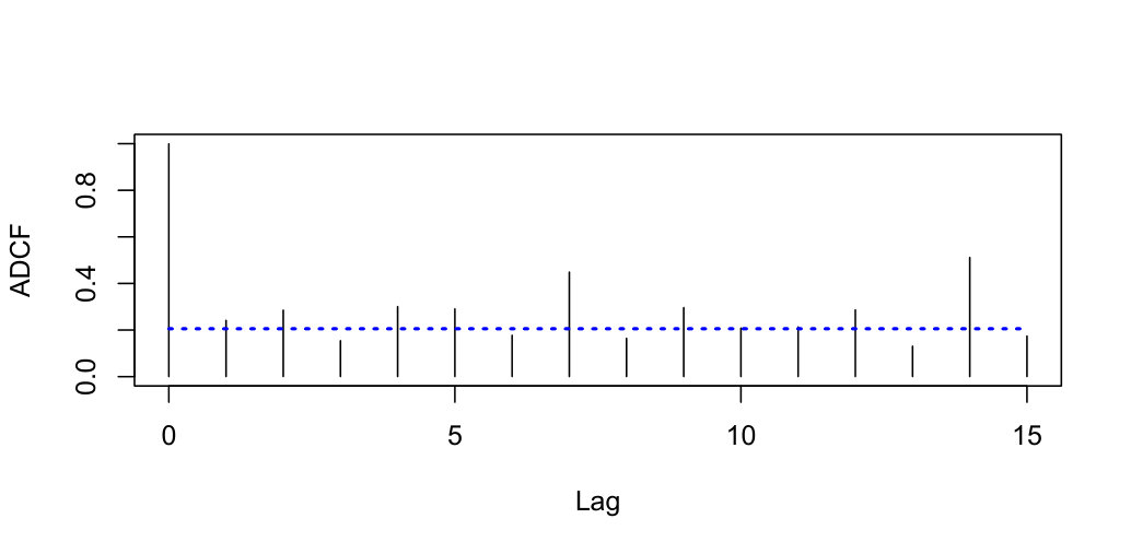 Figure 1
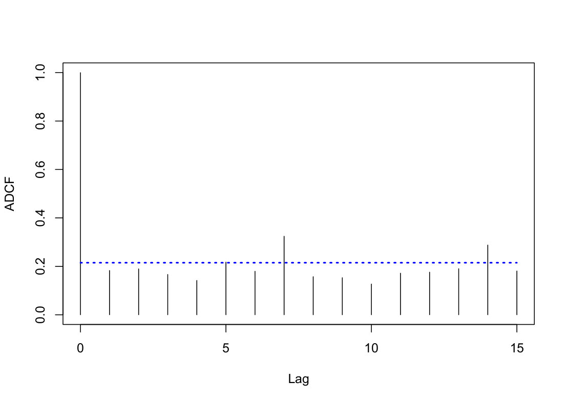 Figure 2
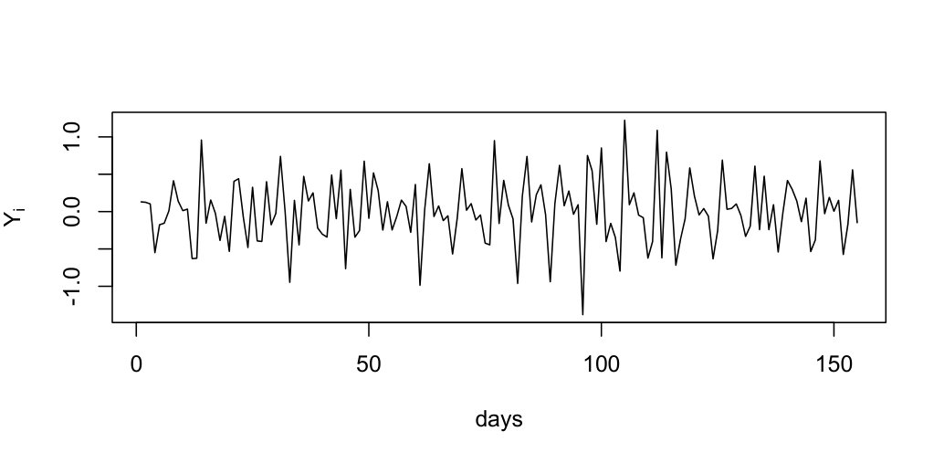 Figure 3
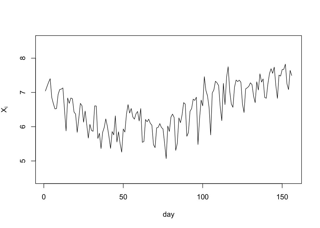 Figure 4
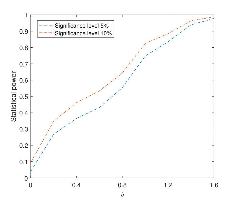 Figure 5
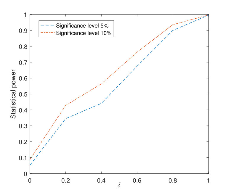 Figure 6
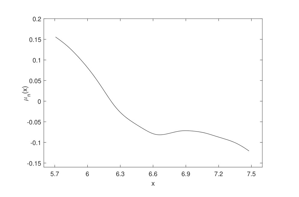 Figure 7
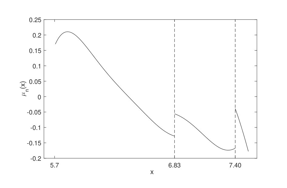 Figure 8
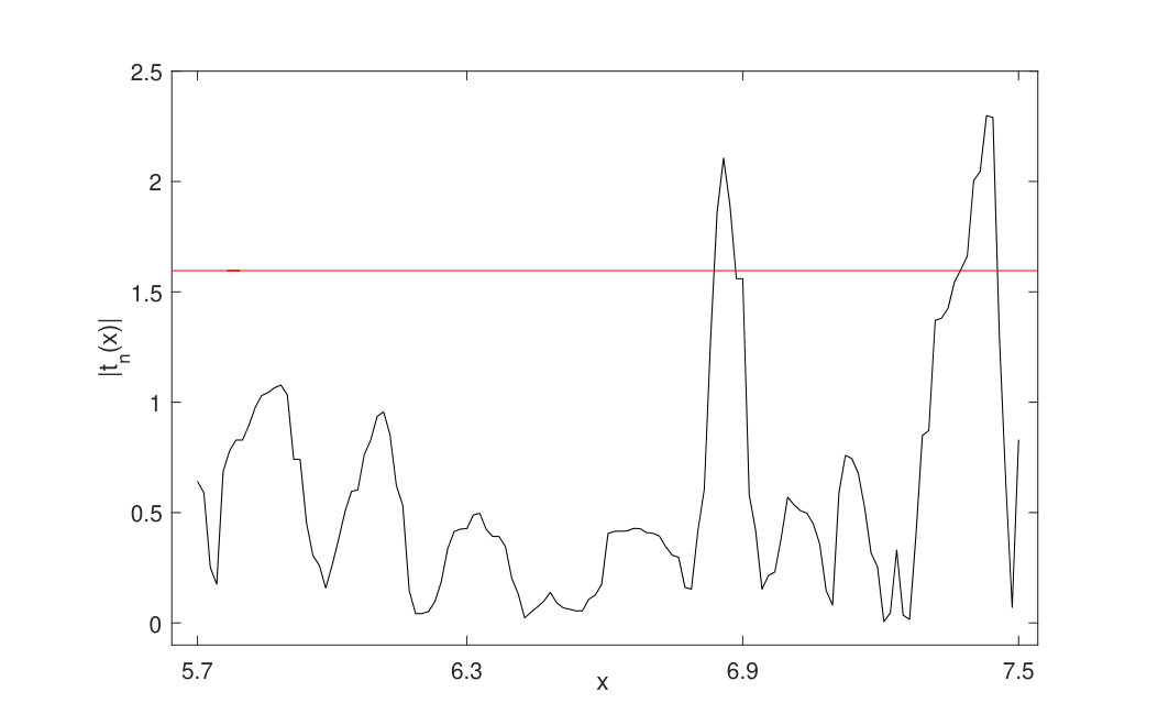 Figure 9
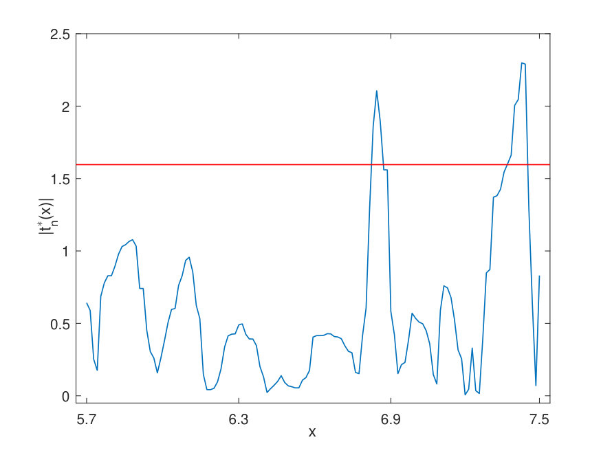 Figure 10
| Model A | 0.2 | 0.4 | 0.6 | 0.8 | |
|---|---|---|---|---|---|
| 0.240 | 0.321 | 0.412 | 0.523 | ||
| 0.046 | 0.055 | 0.064 | 0.067 | ||
| 0.048 | 0.052 | 0.060 | 0.065 | ||
| 0.053 | 0.049 | 0.050 | 0.065 | ||
| 0.103 | 0.109 | 0.132 | 0.131 | ||
| 0.096 | 0.092 | 0.119 | 0.138 | ||
| 0.099 | 0.092 | 0.109 | 0.126 |
| Model | B | C | D | E | ||
|---|---|---|---|---|---|---|
| 0.040 | 0.044 | 0.050 | 0.060 | |||
| 0.066 | 0.041 | 0.054 | 0.054 | 0.195 | ||
| 0.056 | 0.051 | 0.057 | 0.054 | |||
| 0.085 | 0.106 | 0.124 | 0.105 | |||
| 0.102 | 0.092 | 0.114 | 0.092 | 0.258 | ||
| 0.093 | 0.101 | 0.112 | 0.095 | |||
| Case 1 | MADE | MSE | Percentage | |
|---|---|---|---|---|
| =0 | 200 | 0.0451 | 0.0055 | 90.51 |
| 500 | 0.0195 | 0.0014 | 93.77 | |
| 800 | 0.0134 | 0.0006 | 94.51 | |
| Case 2 | MADE | MSE | Percentage | |
| 200 | 0.0519 | 0.0059 | ||
| 0.0757 | 0.0069 | |||
| 500 | 0.0508 | 0.0043 | 86.59 | |
| 0.0496 | 0.0042 | |||
| 800 | 0.0386 | 0.0028 | 89.80 | |
| 0.0362 | 0.0024 |
| 0.5 | 0.3 | 0.1 | |||||
|---|---|---|---|---|---|---|---|
| Para. | 0.042 | 0.175 | 0.831 | 0.904 | 1 | 1 | |
| 0.095 | 0.282 | 0.897 | 0.906 | 1 | 1 | ||
| Nonpara. | 0.069 | 0.256 | 0.406 | 0.646 | 0.792 | 0.910 | |
| 0.131 | 0.378 | 0.540 | 0.761 | 0.861 | 0.940 |
| MADE | MSE | ||
|---|---|---|---|
| Nonpara. | 200 | 0.1055 | 0.0143 |
| 500 | 0.0519 | 0.0066 | |
| 800 | 0.0367 | 0.0041 | |
| Para. | 200 | 0.0340 | 0.0027 |
| 500 | 0.0178 | 0.0012 | |
| 800 | 0.0098 | 0.0004 |
Peer Reviews
No public reviews on file for this paper yet. If you reviewed it on a platform where reviews are public (OpenReview, ICLR, NeurIPS, ICML), you can paste yours below so the community can read it here.
Videos
No videos yet. Explain this paper in a talk, walkthrough, or lecture? Add one.
Taxonomy
TopicsControl Systems and Identification · Advanced Control Systems Optimization
State-domain Change Point Detection for Nonlinear Time Series Regression
Yan Cui1,2
,
Jun Yang3
and
Zhou Zhou1
1 Department of Statistical Sciences, University of Toronto, Canada
2 Institute for Advanced Study in Mathematics, Harbin Institute of Technology, China
3 Department of Statistics, University of Oxford, United Kingdom
Abstract.
Change point detection in time series has attracted substantial interest, but most of the existing results have been focused on detecting change points in the time domain. This paper considers the situation where nonlinear time series have potential change points in the state domain. We apply a density-weighted anti-symmetric kernel function to the state domain and therefore propose a nonparametric procedure to test the existence of change points. When the existence of change points is affirmative, we further introduce an algorithm to estimate the number of change points together with their locations. Theoretical results of the proposed detection and estimation procedures are given and a real dataset is used to illustrate our methods.
Key words: Change-point detection; Nonlinear time series; Nonparametric hypothesis test; State domain.
1. Introduction
Consider the following state-domain nonlinear auto-regression
[TABLE]
where is an unknown regression function, is a martingale difference sequence such that almost surely. Special cases of Eq. 1 include threshold AR models (Tong, 1990), exponential AR models (Haggan & Ozaki, 1981) and ARCH models (Engle, 1982), among others. Furthermore, Eq. 1 can be viewed as a discretized version of the diffusion model
[TABLE]
where is the instantaneous return or drift function, and is a continuous-time martingale. In the literature, the special case of Model \reftagform@2 with has been widely discussed to understand and model nonlinear temporal systems in economics and finance, where denotes the standard Brownian motion and is understood as the volatility function. Among others, Stanton (1997), Chapman & Pearson (2000) and Fan & Zhang (2003) considered the nonparametric estimation of and . Zhao (2011) addressed the model validation problem for Eq. 2. In particular, Eq. 2 can be used to model the temporal dynamics of financial data with being interest rates, exchange rates, stock prices or other economic quantities. Among others, Zhao & Wu (2006) considered kernel quantile estimates of Eq. 2 for the exchange rates between Pound and USD. Liu & Wu (2010) constructed simultaneous confidence bands for and with the U.S. Treasury yield curve rates data. See also the latter papers for further references. Observe that we allow the error process to be general martingale differences in \reftagform@1 which significantly expands the applicability of our theory and methodology in economic applications. As pointed out by one referee, conditional moment restrictions in dynamic economic models routinely arise from Euler/Bellman equations in dynamic programming, which are martingale differences. Furthermore, asset returns, due to the no-arbitrage theory, are (semi)martingales. Hence, their (demeaned) returns are martingale differences.
Throughout this article, following Chapter 6.3 of Fan & Yao (2003), we shall call \reftagform@1 a state-domain nonlinear regression model. The term “state domain” originated from the celebrated state-space models (e.g. Kalman (1960) and Shumway & Stoffer (2000, Chapter 6)) where the dynamics of a sequence of state variables ( in Eq. 1) are driven by a group of control variables ( in Eq. 1) through the nonlinear state equation \reftagform@1. Therefore in this article the term “state domain” refers to the Euclidean space in which the variables on the axes are the state variables. Observe that the state-domain nonlinear regression \reftagform@1 aims to characterize the relationship between and past values (states) of the time series through a discretized stochastic differential equation. On the contrary, time-domain nonlinear regression (see e.g. Fan & Yao (2003), Chapter 6.2)
[TABLE]
with describes the relationship between and time.
To date, most investigations on the nonparametric inference procedure of Eq. 1 are based on the assumption that the underlying regression function is continuous, which may cause serious restrictions in many real applications. In fact, in parametric modeling of nonlinear time series, various choices of with possible discontinuities have drawn much attention in the literature. One of the most prominent examples is the threshold model proposed by Tong & Lim (1980), in which regime switches are triggered by an observed variable crossing an unknown threshold. Also, AR model with regime-switch controlled by a Markov chain mechanism was introduced by Tong (1990). In economics, the expanding phase and contracting phase are not always governed by the same dynamics, see Tiao & Tsay (1994); Durlauf & Johnson (1995); McConnell & Perez-Quiros (2000) and other references therein. As a result, the occurrence of abrupt changes in the state-domain regression function is common and detecting as well as estimating them are of vital importance. Motivated by this, in the current paper we focus on the situation where the regression function is piece-wise smooth on an interval of interest with a finite but unknown number of change points. More precisely, there exist such that is smooth on each of the intervals ; that is, on the interval
[TABLE]
where is the total number of change points. Throughout this article, we assume is fixed.
To our knowledge, there exist no results on change point detection of the state-domain regression function in the literature. The purpose of this paper is twofold. First we want to test whether is smooth or discontinuous on the interval ; that is to test the null hypothesis of Eq. 4. By sliding a density-weighted anti-symmetric kernel through the state domain, we shall suggest a nonparametric test statistic and non-trivially apply the discretized multivariate Gaussian approximation result of Zaitsev (1987) to establish its asymptotic distribution. Additionally, the Gaussian approximation results also directly suggest a finite sample simulation-based bootstrapping method which improves the accuracy of the test in practical implementations. Second, if , we reject the null hypothesis and subsequently want to locate all the change points. In this case, we propose an estimation procedure and establish the corresponding asymptotic theory on the accuracy of the estimators. Finally, the above theoretical results are of general interest and could be used for a wider class of state-domain change point detection problems.
There is long-standing literature in statistics discussing jump detection of the time-domain nonlinear regression model \reftagform@3 where occasional jumps occur in an otherwise smoothly changing time trend . It is impossible to show a complete reference here and we only list some representative works. Müller (1992) and Eubank & Speckman (1994) employed a kernel method to estimate jump points in smooth curves. Wang (1995) suggested using wavelets and provided a review of jump-point estimation. Two-step methods were considered by Müller & Song (1997) and Gijbels et al. (1999) to study the asymptotic convergence properties of the jumps. Later, Gijbels et al. (2007) suggested a compromise estimation method which can preserve possible jumps in the curve. Zhang (2016) considered the situation where the trend function allows a growing number of jump points. In econometrics, there is a significant body of literature discussing time-domain jump detection in jump diffusion models; see for instance Bollerslev et al. (2008); Jiang & Oomen (2008); Lee & Mykland (2012) and the references therein. On the other hand, it is well known that state-domain asymptotic theory is very different from that of the time domain (see, for instance Fan & Yao (2003), Chapter 6). In our specific case, uniform asymptotic behavior of our test statistic on is arguably more difficult to establish than the corresponding problem in the time domain. In the current paper, we establish that, unlike time-domain change point detection problems of \reftagform@3 where the long-run variances of the process are of crucial importance in the asymptotics, state-domain change point detection theory of \reftagform@1 heavily depends on the conditional variances and densities of the process . We also provide an estimation procedure using simulated critical values to detect and locate the change points. We show that, when the jump sizes have a fixed and positive lower bound, the method will asymptotically detect all the change points with a preassigned probability and an accuracy which is much smaller than , where is the length of the time series.
The rest of the paper is organized as follows. In Section 2, we introduce the model framework and some basic assumptions. Section 3 contains our main results, including a nonparametric test to determine the existence of change points and a procedure for estimating the number of change points together with their locations. Practical implementation based on a bootstrap procedure and a suitable method for bandwidth selection are discussed in Section 4. Section 5 reports some simulation studies. A real data application of daily COVID-19 infections in Germany is carried out in Section 6. Section 7 contains all the proofs of the theoretical results in Section 3.
2. Model Formulation and Basic Assumptions
Throughout this paper, we use the following notations. A random vector if . For two random variables and , denotes the conditional distribution function of given and denotes the conditional density. Furthermore, for function with , we let be the conditional expectation of given . Finally, stands for the indicator function.
Assume that the process is stationary and causal. Following Wu (2005), we assume that is a Bernoulli shift process such that
[TABLE]
where the function is a measurable function such that the process exists and is a shift process, where are independent and identically distributed (i.i.d.) random variables. Furthermore, is a martingale difference sequence satisfying almost surely. From Eq. 5, one can interpret the transform as the underlying physical mechanism, with and being the input and output of the system, respectively.
Similarly, we assume
[TABLE]
where is a measurable function such that exists. To facilitate the main results, we first introduce the time series dependence measures in Wu (2005) associated with and . Assume , and let
[TABLE]
where is a coupled process of with replaced by an i.i.d. copy . Then, we define the physical dependence measures of as
[TABLE]
Let if . Thus for measures the dependence of the output on the single input . We refer to Wu (2005) for more details on the physical dependence measures.
Similarly, we define the physical dependence measures for the errors as
[TABLE]
where . Let if .
Suppose that is observed. Recall and we aim to test the null hypothesis that the regression function is smooth. To this end, we introduce a density-weighted anti-symmetric kernel function , which is defined by
[TABLE]
where is a kernel function supported on with and . The data-dependent weights and are defined by
[TABLE]
where is the bandwidth satisfying and . Note that and are one-sided kernel density estimators. Hence can be approximated by , where is the density function of . Observing that is an anti-symmetric function, we then call a density-weighted anti-symmetric kernel function. By sliding this kernel function through the state domain, we are able to test whether has change points. More specifically, the quantity is a boundary kernel estimation of , where and are the right and left limits of at . Thus, if is a continuous point of , this quantity will be approximately zero at . However, if is discontinuous at , the quantity will be approximately equal to the jump size of at . To establish our first main result, we need the following regularity conditions:
- (a)
There exist such that and . 2. (b)
Assume where . 3. (c)
For the same defined in Condition (b), assume that , , and for some . 4. (d)
The density function of is positive on for some and there exists a constant such that
[TABLE] 5. (e)
is differentiable over , the right derivative and the left derivative exists and . The Lebesgue measure of the set is zero. Furthermore, and .
For the above regularity conditions, Condition (a) specifies the allowable range of the bandwidth. Condition (b) puts a mild moment restriction on . Condition (c) requires that the quantities and satisfy the geometric moment contraction (GMC) property. The GMC property is preserved in many linear and nonlinear time series models such as the ARMA models and the ARCH and GARCH models; see Shao & Wu (2007) for more discussions. Furthermore, denote , which measures the cumulative dependence of on . Then if Condition (c) holds, it is easy to see that which indicates short-range dependence of . With Condition (d), we require that the density and conditional density of exist and are bounded. Moreover, has bounded derivatives up to the second order. Condition (e) puts some restrictions on the smoothness and order of the kernel function . In particular, indicates that is a second-order kernel which has both positive and negative parts on .
3. State-domain Change Point Detection and Estimation
In this section, we propose a test on the existence of change points in and an algorithm to estimate the number and locations of the change points when is discontinuous.
3.1. Test for the existence of change points.
With the foregoing discussion, we introduce a nonparametric statistic based on the density-weighted anti-symmetric kernel to test whether model Eq. 1 has change points in the state domain regression function on . By proper scaling, our test statistic is defined as
[TABLE]
where . In practice, since and are unknown, we use the kernel density estimator and Nadaraya–Watson (NW) estimator to replace and , respectively. The kernel density estimator is given by
[TABLE]
where is a general kernel function with and is the bandwidth sequence satisfying and . Let be the square of the estimated residuals, where
[TABLE]
is the NW estimator of , then the NW estimator of is given by
[TABLE]
The following remark provides the uniform consistency of the estimated density and conditional variance functions.
Remark 3.1*.*
Under Condition (a) for both bandwidths and with , Condition (c), Condition (d), and Condition (e), we have
[TABLE]
where and
[TABLE]
Similarly, for , under the conditions of Theorem 3.2, we also have
[TABLE]
See Section 8.1 for the proof.
Let be the density function of and . We have the following main result on the asymptotic properties of the proposed test statistic.
Theorem 3.2**.**
Let be fixed. Recall the piece-wise formulation of Eq. 4, let and be the -neighborhoods of the intervals and , respectively. Let be the collection of the change points, be the -neighborhood of . Assume that Condition (a)-Condition (e) hold with for some and satisfies
[TABLE]
then
[TABLE]
where and
[TABLE]
with .
Proof.
See Section 7.1. ∎
Theorem 3.2 is a general result which establishes the asymptotic theory of the test statistic. In practical implementation, we will use the density estimates and variance estimates instead of and to calculate as discussed before. Therefore, we have the following corollary.
Corollary 3.3**.**
Denote . Under the conditions of Theorem 3.2 and further assume the bandwidth , then the asymptotic result of Theorem 3.2 holds for ; this is
[TABLE]
Note that in Corollary 3.3, we have added the assumption with the purpose of ensuring the consistency of and on . When there is no change point in , we have similar results as shown in the following remark, which suggests that under the null hypothesis, after proper scaling and centering, our test statistic converges to a Gumbel distribution asymptotically.
Remark 3.4*.*
Assume holds. We further assume that and the remaining conditions of Corollary 3.3 hold. Then, , , which implies . Therefore, the previous theorem reduces to
[TABLE]
Denote the jump-size of at as ; that is, . Next, we consider the alternative hypothesis with . When holds true, it is easy to see that the proposed test has an asymptotic power as . In other words, with some preassigned level and as , we have
[TABLE]
Once the null hypothesis of no change point is rejected, one would be interested in detecting the number of change points together with their locations, which we discuss in Section 3.2.
3.2. Change-point Estimation
Suppose there exist a fixed number of change points on , which are denoted by , with the minimum jump size . In this paper, we assume which is allowed to decrease with . The idea for estimating the number and locations of the change points is to search for local maximas of which exceed the critical value of the test. To be more specific, we propose in the following a procedure for change point estimation.
- •
For a fixed level , perform the bootstrap procedure described in Section 4.1 to determine the critical value, say .
- •
Set .
- •
Starting from the interval , find the largest of that exceeds the critical value and denote its location as , then rule out the interval from to get .
- •
Repeat the previous step until all significant local maximas are found. In other words, on the remaining intervals are all below .
- •
Denote the number of detected change points by and re-order the estimated change points as .
The following theorem provides an asymptotic result for and .
Theorem 3.5**.**
Under the conditions of Theorem 3.2, we further assume that is differentiable over with , the right derivative and the left derivative exist and . The Lebesgue measure of the set is zero. If then for any given level , we have
[TABLE]
for any such that
Proof.
See Section 7.2. ∎
Theorem 3.5 reveals that for any given small probability , with asymptotic probability , our proposed procedure will correctly estimate all the change points with an accuracy . It is important to mention that when , that is, when the jump sizes have a fixed lower bound, the smallest order for is , which is smaller than . It can also be seen as a product of and the optimal convergence rate of time-domain change-point estimators established in Müller (1992). Hence, we conjecture that our rate is nearly optimal for state-domain change point detection.
4. Practical Implementation
4.1. The bootstrap procedure
It is well known that the convergence rate of the Gumbel distribution in Theorem 3.2 is slow. As a result, a very large sample size would be needed for the approximation to be reasonably accurate. To overcome this issue, we propose a simulation-based bootstrap procedure to improve the finite-sample performance of the proposed test. The bootstrap procedure is as follows.
- •
Generate i.i.d. standard normal random variables .
- •
Compute the quantity defined in Eq. 26 for many times and calculate its th quantile as the critical value of our test.
For the proposed boostrap procedure, we have the following theoretical results which shows that, with proper scaling and centering, has the same asymptotic Gumbel distribution.
Proposition 4.1**.**
Denote and
[TABLE]
where are i.i.d. standard normal random variables and is its density. Assume , Condition (a), Condition (e) hold and satisfies
[TABLE]
Then we have
[TABLE]
Proposition 4.1 shows that and have the same asymptotic Gumbel distribution with proper scaling and centering under the null hypothesis. Therefore, the th quantile of can be estimated consistently by calculating the empirical th quantile of with a large number of replications by the bootstrap procedure. We reject the null hypothesis at level if . When implementing the procedure described in Section 3.2 for estimating the change points, we also suggest using to find the detection region. Our numerical experiments suggest that the bootstrap method yields more accurate results than those based on the asymptotic limiting distribution under small or moderate sample sizes.
4.2. Bandwidth selection
The bandwidth used in can be chosen based on classic bandwidth selectors for nonparametric kernel density estimation. However, the choice of bandwidth for test statistic and for the estimated variance can be quite nontrivial and are usually of practical interest. In this paper, we adopt the standard leave-one-out cross-validation criterion for bandwidth selection suggested by Rice & Silverman (1991):
[TABLE]
where and are the kernel estimators of and computed with all measurements with the th subject deleted, respectively. For example, a cross-validation bandwidth can be obtained by minimizing with respect to , i.e., , where is the allowable range of . The bandwidth selection for is similar.
5. Simulation Study
In this section, we carry out Monte Carlo simulations to examine the finite-sample performances of our proposed test and estimator. Throughout the numerical experiments, the Epanechnikov kernel is used for estimating the density and conditional variances. On the other hand, we adopt the higher-order kernel function in the form in the expression of , where is the kernel function on [0,1] by shifting and scaling . From Theorem 3.2, one can see that the power of our test increases as decreases. As a result, we aim to maximize the quantity with the constraints and to choose and . It turns out that is maximized at and . Hence, we will use in our simulations and data analysis.
5.1. Accuracy of bootstrap.
We run Monte Carlo simulations to study the accuracy of the proposed bootstrap procedure for finite samples and 800. Here, we aim to test the null hypothesis of no change point in the regression function. The number of replications is fixed to be 1000 and the number of bootstrap samples is at each replication.
To guarantee the stationarity of the process , is required to be less than one (Fan & Yao, 2003, Section 2.1). First, we consider Model A listed below to investigate the robustness of our testing procedure with respect to various levels of persistence in the data generating process. Additional four state-domain nonlinear models (Models B - E listed below) where is of various shapes are further investigated for the accuracy of our test. In our simulations the martingale difference process with and . Note that the error processes are specified via different conditional variance functions in Models A–D. On the other hand, in Model E we set where so that has a period of 7 which matches the data generating process observed in the empirical data example in Section 6.
- •
Model A:
[TABLE]
where represents various levels of temporal dependence in the series.
- •
Model B:
[TABLE]
- •
Model C:
[TABLE]
- •
Model D:
[TABLE]
- •
Model E:
[TABLE]
Note that the regression functions in Models A–E are all continuous. At nominal significance levels and , the simulated Type I error rates for sample sizes and are reported in Tables 1–2 for Model A and Models B–E, respectively. To measure the strength of the nonlinear temporal dependence, we will employ the auto-distance correlation function (ADCF) investigated in Zhou (2012). In Table 1, we illustrate the first order ADCF (denoted by ) for Model A. Meanwhile, for Model E the first order and the seventh order ADCF are listed in Table 2. One can see that the performance of our testing procedure is reasonably accurate for different sample sizes across the models and the accuracy improves as the sample size increases. On the other hand, from Table 1, we find that as the dependence of the process becomes stronger, the type I errors tend to be less accurate, but are still in a reasonable range.
5.2. Power of hypothesis testing
In this subsection, we consider the simulated power of our test under various alternatives. Recall the representation with . Here, we consider the following two types of alternatives with a change point of size :
- •
Model F1:
[TABLE]
- •
Model F2:
[TABLE]
We let the jump size range from [math] to for model F1 and from [math] to for model F2 at location . For each model, we investigate the empirical sensitivity of our testing procedure under nominal levels and with sample size based on replications. The simulated power curves for the above models are plotted in Fig. 1 and Fig. 2, respectively. According to the plots, the statistical power of the proposed testing procedure increases reasonably fast as increases. On the other hand, we also observe that our test shows a slower speed of increase at near alternatives when compared with “classic” power curves of parametric tests. We believe that part of the reason is that our nonparametric test aims at detecting alternatives from a large class of discontinuous functions while tests tailored to some parametric models (such as the threshold model) target a specific class of alternative functions. Therefore our test is expected to be less sensitive to small deviations from the null compared to those parametric tests. See also Section 5.4 for a numerical experiment that compares the sensitivity of our testing procedure with that of a parametric test of the threshold model.
5.3. Accuracy in estimating the number of change points and their locations
Utilizing the algorithm listed in Section 3.2, in this subsection we focus on estimating the number of change points and their locations based on realizations with sample sizes and . In the simulations, we let the error process be i.i.d. standard normal random variables and consider the following two cases:
- •
Case 1: A single change point.
[TABLE]
- •
Case 2: Two change points.
[TABLE]
The estimates of the locations of change points are compared in terms of their mean absolute deviation errors (MADE) and mean squared errors (MSE). We also report the simulated percentage of correctly estimating the number of change points. The results are listed in Table 3. One can see from Table 3 that the values of MADE and MSE are all quite small, which suggests the estimated locations by our approach are fairly accurate. Furthermore, as the sample size increases, the percentage of correctly estimating the number of change points increases in both cases.
5.4. Comparison to threshold testing and estimation in threshold model
In this subsection, we compare the accuracy and sensitivity of our nonparametric method with existing threshold testing and estimation methods for the classic threshold AR (TAR) model proposed by Tong & Lim (1980) when the TAR model is indeed the underlying data generating mechanism. We consider the following two-regime TAR(1) model
[TABLE]
where and the error process . First, we are interested in comparing the accuracy and power of our nonparametric test with the parametric -test of threshold nonlinearity proposed in Tsay (1989). Table 4 shows the testing results for nonlinearity of the model based on both the parametric and nonparametric methods, in which the sample size is and the number of bootstrap samples is .
We observe that the nonparametric method has slightly higher powers when the scale coefficient changes slightly from 0.5. However, as becomes or smaller, the parametric method has higher powers than the nonparametric method.
In addition, we compare the accuracy in change point estimation. We study the following TAR(1) model,
[TABLE]
where . Note that parametric estimation of the threshold value of the above two-regime TAR(1) process can be done via the R function uTAR in the NTS package (we refer to Liu et al. (2020) for more details). The simulated MADEs and MSEs are listed in Table 5. From Table 5, one can see that both methods provide relatively accurate estimates of the locations of change point (threshold). The parametric method shows more accurate estimation results comparing with those of the nonparametric method. With the above observations, it can be seen that the parametric method is better for testing and detecting change points for the TAR model when the model is well-specified. This result is not surprising since testing sensitivity and estimation accuracy tend to be higher when the model is correctly restricted to a (smaller) parametric class.
6. Illustrative example
In this section, we consider the daily new confirmed cases of Coronavirus disease of 2019 (COVID-19) in Germany. The dataset contains observations from April 28th to September 30th of 2020 which can be downloaded from https://ourworldindata.org/coronavirus-source-data. From the COVID-19 timeline, Germany registered the first case on January 28th and later suffered an outbreak of this pandemic from mid March to late April. In the data analysis, we select the aforementioned time span between the first and second waves of COVID-19 so that the time series is approximately stationary. Let be the logarithm of confirmed cases at day and . The sample path of and the ADCF plot of are shown in LABEL:F3. Both plots in LABEL:F3 suggest that the time series is approximately stationary and has a moderate seasonal dependence with period . The seasonal behaviour probably comes from the reporting lag behind during weekends, which happens in almost every country. We consider the state-domain nonlinear regression model (which is equivalent to Eq. 1):
[TABLE]
where is a martingale difference sequence. In this application, represents the expected increase or decrease in percentage of COVID-19 cases in day when .
We apply the proposed method to testing whether contains any change points. We choose which includes 82.69 of so that data are relatively abundant in this region and the test is expected to be accurate. According to the leave-one-out cross-validation criterion, the selected bandwidths and are and , respectively. Through the practical implementation in Section 4.1, we calculate the empirical 99 quantile of with 10000 bootstrap samples, which gives . Next, we investigate the behaviour of the test statistics, which is shown in Fig. 4. Our test rejects the null hypothesis of continuity of at level and flags two change points at and .
Note that can be viewed as the conditional daily growth rate for COVID-19. For comparison, we also use the nonparametric local polynomial method to fit assuming that there is no change point. The corresponding estimated regression function over is plotted on the left hand side of Fig. 5. On the right hand side of Fig. 5 we plot the fitted drift function with the knowledge of the change points. The difference between the two plots in Fig. 5 suggest that, with or without the knowledge of change points, our understanding of the relationship between and can be quite different. With the knowledge of the change points, we can see that two large jumps exist at and , which shows that the growth rate changes abruptly at these two points.
It is obvious to see from the right plot of Fig. 5 that those two change points divide the state domain into three regimes/phases. Furthermore, the latter plot indicates that the nonlinear dynamics can be approximated by a three-regime threshold model with the data generating mechanism switching at the detected change points. Additionally, according the timeline, we can find out the periods corresponding to each phase. The first phase contains May 3-5, 10-11, May 15-August 5, August 9-10, 16-17, 23-24 and 30-31 where the trajectory depicts a relatively inactive period of the virus transmission and the conditional infection rate decreases from positive to negative as increases. The second phase includes April 28-30, May 6-9, August 7-9, 11-15, 25-29, September 1-6, 8-9, 13-15 and 20-21 where the conditional infection rate jumps up when surpasses and then it decreases gradually again. The third phase corresponds to August 20-21, September 16-19 and 22-26 where a sudden large increase in the conditional infection rate can be found at the left boundary and then it decreases sharply, possibly due to strong governmental interventions.
In summary, the analyzed period from April 28th to September 30th of 2020 of German COVID-19 data shows a complicated nonlinear dynamic balance between disease transmission and government intervention. The proposed method of the paper could help understand this complex nonlinear dynamics by determining the boundaries of phases where the state-domain relationship changes abruptly and subsequently segment the time series into multiple regimes.
Acknowledgments. The authors are grateful to the editor, Prof. Serena Ng, and two anonymous referees for their valuable comments and suggestions which significantly improved the quality of the paper. Zhou Zhou’s research has been partially sponsored by NSERC (No.489079). Yan Cui is supported by the China Scholarship Council (No.201806170148).
7. Proofs of main results
7.1. Proof of Theorem 3.2
The outline of the proof is as follows. Firstly, we use the following decomposition of
[TABLE]
and prove the results involving the first two terms. This is given in Section 7.1.1.
Secondly, we use a technique called -dependent approximation to approximate the martingale using , where , for a properly chosen order , which simplifies the sum of a sequence of dependent random variables to a corresponding sum of -dependent random variables. This is done in Section 7.1.2.
Thirdly, we divide the sequence of (-dependent) random variables into alternating big and small blocks, where the length of big blocks has a slightly higher order than that of the small blocks. Furthermore, the length of the small blocks is larger than . Using this proof technique, we can approximate the sum of (-dependent) random variables using the sum of the subsequence which includes the random variables residing in the big blocks. Since the length of small blocks is larger than , the -dependent random variables in different big blocks are independent. This part of the proof is given in Section 7.1.3.
Fourthly, we only need to deal with a sequence of independent sums of random variables within each big block. In order to get prepared for using the multivariate Gaussian approximation result by Zaitsev (1987), we first compute the asymptotic covariance structure of the sequence of independent sums. This is given in Section 7.1.4.
In the final two steps, we first apply the multivariate Gaussian approximation by Zaitsev (1987), which is given in Section 7.1.5 and then prove the convergence to Gumbel distribution, which is given in Section 7.1.6. The techniques used in these two steps heavily depend on some existing work, particularly, the work by Zhao & Wu (2008); Liu & Wu (2010), which eventually applied the work by Bickel & Rosenblatt (1973); Rosenblatt (1976).
7.1.1. Decomposition
First, we substitute into and separate the terms involving and . We first focus on the term involving only. That is,
[TABLE]
Next it is easy to see that by the definition of , the second term of the decomposition on the right hand side of Eq. 41 equals . For the first term of the decomposition in Eq. 41, following exactly the proof of (Liu & Wu, 2010, Lemma 5.2), uniformly over , we have that
[TABLE]
where comes from (Zhao & Wu, 2008, Lemma 2(ii)), and in the last equality we have applied the assumptions on and to get .
7.1.2. -dependent approximation
For the third term of the decomposition in Eq. 41, recalling that we have defined the notation , we consider the decomposition of ,
[TABLE]
where where . The first and last terms in the decomposition can be ignored comparing to the second term. To see this, consider
[TABLE]
which implies . Since , we have
[TABLE]
Similarly, one can verify in the same way that
[TABLE]
Furthermore, since the martingale differences are uncorrelated, we have
[TABLE]
Therefore, defining
[TABLE]
we have
[TABLE]
Next, following exactly the proof of (Liu & Wu, 2010, Lemma 5.3), we get that uniformly over
[TABLE]
Following the above arguments again we can compute the orders for the decomposition of the term involving and get by the differences. Note that many terms such as in the second term and term in the first term cancel out. Therefore, overall it can be easily verified that
[TABLE]
where is an anti-symmetric kernel defined by
[TABLE]
Now to prove Theorem 3.2, it suffices to show
[TABLE]
where
[TABLE]
Note that we have and . Next, we define a truncated version of by
[TABLE]
We next define using -dependent conditional expectations
[TABLE]
where .
7.1.3. Alternating big and small blocks
Recall that . We choose such that and split into alternating big and small blocks with length , , , and . Note that . Then we define
[TABLE]
Then we define
[TABLE]
Next we show in the following that we can approximate by and then approximate by . That is, we show
[TABLE]
To show LABEL:{lemma_approximate_Mn}, we first follow the proof of (Liu & Wu, 2010, Lemma 5.1) using Freedman’s inequality for martingale differences Freedman (1975) to get
[TABLE]
which implies we can approximate by replacing with in the definition of .
Next, we write as a sum of three terms
[TABLE]
Note that is uncorrelated with the second term of the right hand side of Eq. 64. Next, we show that under our assumptions on physical dependence measure, the first term of the right hand side of Eq. 64 becomes very small for large . In order to rigorously prove this fact, defining
[TABLE]
we first approximate by the skeleton process , where and . Following the same arguments as in (Liu & Wu, 2010, Proof of Lemma 4.2) using Freedman’s inequality for martingale differences Freedman (1975), we have
[TABLE]
Next, we show exponentially decays with . We consider two cases and , where . Using the assumption , we have
[TABLE]
Now, we can show the maximum of the skeleton process over is small. Recall that is a polynomial of , then we have
[TABLE]
Next, we show the third term of the decomposition of in Eq. 64 can also be ignored. In order to show this, we define
[TABLE]
Using the same argument as in (Liu & Wu, 2010, Proof of Lemma 4.2), we can approximate by its skeleton process, since . We first approximate by the maximum over the skeleton process. Then we have using Freedman’s inequality for martingale differences Freedman (1975). Therefore, we can approximate by
[TABLE]
Furthermore, since , we can replace by , which leads to the definition of . Therefore, we have proved
[TABLE]
Therefore, in order to finish the proof of Eq. 62, it suffices to show
[TABLE]
where . Following the same argument as above using skeleton process, we only need to consider the grids . Using the fact that and , again by Freedman’s inequality for martingale differences, for some constant that
[TABLE]
which finishes the proof of Eq. 62.
Observing that, since is supported on , one of the following two terms must be zero:
[TABLE]
Hence, defining similarly as using instead of , by Eq. 62, we only need to focus on the following term
[TABLE]
Clearly, in order to complete the proof of Theorem 3.2, it suffices to show
[TABLE]
7.1.4. Asymptomatic covariance structure
Next, we prove some results on the asymptomatic covariance structure of which will be needed later for Gaussian approximation using the results in Bickel & Rosenblatt (1973). Define the following quantities: , , , and . Note that since , we have . Then by the definition of , using , we have
[TABLE]
Next, according to (Bickel & Rosenblatt, 1973, Theorems B1 and B2), we have . Note that
[TABLE]
This implies , which can also be obtained directly from (Bickel & Rosenblatt, 1973, Theorems B1 and B2).
Next, we show . Note that are uncorrelated and . Then, using uniformly over and , we have
[TABLE]
Therefore, we have proved that, as ,
[TABLE]
7.1.5. Gaussian approximation
Now, we go back to prove Eq. 77. We use similar techniques as in (Liu & Wu, 2010, Proof of Lemma 4.5). First, as in Bickel & Rosenblatt (1973), we split the interval into alternating big and small intervals , where , , , and . We let be fixed, and be small which goes to [math]. Since and are fixed numbers, without loss of generality, we assume and in this proof.
Next, we approximate by big blocks . That is, by , where . Then we further approximate via discretization by , where with . We define , , , and similarly by replacing or by or , respectively. Letting and , we have
[TABLE]
where
[TABLE]
Next, we are ready to apply Gaussian approximation. We first use discretization for approximating . Let , where , . Write , where and . Following the same arguments as in (Liu & Wu, 2010, Proof of Lemma 4.6), we have the following discretization approximation holds for all large enough ,
[TABLE]
Next, we apply the multivariate Gaussian approximation from Zaitsev (1987). To this end, similar to the definition of , we first define
[TABLE]
Note that the sequence of random variables are independent. Then we define
[TABLE]
Now we introduce . Then using (Zaitsev, 1987, Theorem 1.1) as well as for large enough , we have
[TABLE]
where is a centered Gaussian random vector with covariance matrix .
Let be the density function of standard Gaussian, and be the Pickands constants (Bickel & Rosenblatt, 1973, Theorem A1, Lemma A1, and Lemma A3). Using Eq. 85, let be such that . Following exactly the arguments in (Liu & Wu, 2010, Proof of Lemma 4.6) to apply (Bickel & Rosenblatt, 1973, Lemma A3 and Lemma A4), we can obtain that for ,
[TABLE]
uniformly over . The limit when also holds, that is
[TABLE]
where we have used the Pickands constants . The left tail version of the tail bounds also holds with replaced by . Furthermore, we can show through elementary calculations that
[TABLE]
Therefore, it suffices to show the following convergence to Gumbel law
[TABLE]
7.1.6. Convergence to Gumbel distribution
The main steps of the proof of Eq. 100 are as follows. First, we approximate by . Then, we approximate by another quantity which is defined similarly to but using a sequence of i.i.d. random variables instead of the dependent time series . Finally, we apply (Rosenblatt, 1976, Theorem) to show convergence to Gumbel distribution.
We define
[TABLE]
where is a centered Gaussian process with covariance function
[TABLE]
First we approximate using . Recall that and are the lengths of big and small blocks and . Let . Define a different truncation order for by for given , where
[TABLE]
Then using and following exactly the same proof from (Liu & Wu, 2010, Proof of Lemma 4.10) to get that, for any fixed integer that ,
[TABLE]
where , , does not depend on , and
[TABLE]
Next, we construct in the following way. Let be i.i.d. copies of , and . Let . Note that are i.i.d. Now define the same as except by replacing and with and , respectively. Repeat the previous arguments for getting Eq. 104, we have
[TABLE]
Letting then , by triangle inequality, we have
[TABLE]
Now the key observation is that we can deal with now and are defined using which are i.i.d. Next, we define to the same as to except using and instead of and , then by Eq. 98 and elementary calculations again we have for . This implies
[TABLE]
where is defined in the same way as by replacing with , and with . Finally, since are i.i.d., we can apply (Rosenblatt, 1976, Theorem), which leads to the convergence of to . This completes the proof of Theorem 3.2.
7.2. Proof of Theorem 3.5
First, let and be positive sequences, then if . On the other hand, if both and hold. Note that
[TABLE]
We first argue that , which implies at least one change point hasn’t been detected, then we can write
[TABLE]
Then, by the validity of the bootstrap procedure, when , the power of the test goes to as which implies that for any ,
[TABLE]
This conclude that .
Next we argue that . Note that implies there is a set without any change point in it, however, . Note that by our algorithm, we can consider to be the largest set constructed by ruling out intervals from such that each interval has length and contains one change point. Then since is a fixed constant and , we have . Then we can apply our main result Theorem 3.2 again on to get that , which implies .
Therefore, we have . Then it suffices to show
[TABLE]
Since is finite, we only need to focus on one change point. Let be any of the true change point and be its estimate, it suffices to show . Without loss of generality, we assume and . The case can be shown using similar arguments. Now we follow similar arguments as in Müller (1992). Define , for . Then we can write . Therefore, it suffices to show . Suppose is small enough such that the -neighborhood of does not include any other change points, then we apply the previous decomposition in Eq. 41. Note that since is a change point, without loss of generality, we assume is left continuous at , then the following term has the order of :
[TABLE]
Furthermore, using because of , considering cases and separately, we have
[TABLE]
Finally, by the assumptions on in Theorem 3.5, we can follow the same arguments in the proof of Theorem 3.2 as the -dependent approximation Section 7.1.2 and alternating big/small blocks Section 7.1.3 applying to instead of to get
[TABLE]
Furthermore, using the fact that is uniformly bounded and mean value theorem, we have
[TABLE]
Next, we define a new kernel such that
[TABLE]
so we have . Then we can approximate the following term using the same arguments of -dependent approximation and alternating big/small blocks as in Section 7.1.2 and Section 7.1.3 in the proof of Theorem 3.2 applying to this new kernel to get
[TABLE]
Therefore, we have
[TABLE]
Then using we can conclude that
[TABLE]
Recall that the estimated change point , where , then we have
[TABLE]
whenever and . This is always true since we have assumed which implies so . Therefore, if we choose such that , then we have , which implies .
8. Additional proofs
8.1. Proof of
For , we first write it as the sum of three terms:
[TABLE]
For the first term, we first approximate by where with small enough. Using the same argument as in Section 7.1, we have
[TABLE]
where we choose with . We then divide into blocks indexed by . Then it’s clear that the sum of blocks with odd indices is independent with the sum of blocks with even indices. Following the same argument as the proof of (Liu & Wu, 2010, Theorem 2.5) for each subsequence of the blocks, and use a union bound, we can get
[TABLE]
For the second term, we first approximate using , where . Then following the same argument as in Section 7.1 we have
[TABLE]
Then, again choosing and divide into blocks, by the same argument as in (Zhao & Wu, 2008, pp. 1875), we can get
[TABLE]
Finally, for the last term, we have
[TABLE]
Then, using we have that
[TABLE]
For , similarly, by the same arguments as the proof for , following the proof of (Liu & Wu, 2010, Lemma 4.4), we can obtain .
8.2. Proof of Proposition 4.1
Since are i.i.d. standard Gaussian distributed random variables, the proof for this proposition is simpler than Theorem 3.2. We can immediately prove the convergence to Gumbel distribution by using (Rosenblatt, 1976, Theorem 1).
The reference list from the paper itself. Each links out to its DOI / PubMed record.
- 1(1)
- 2Bickel & Rosenblatt (1973) Bickel, P. J. & Rosenblatt, M. (1973), ‘On some global measures of the deviations of density function estimates’, The Annals of Statistics 1 (6), 1071–1095.
- 3Bollerslev et al. (2008) Bollerslev, T., Law, T. H. & Tauchen, G. (2008), ‘Risk, jumps, and diversification’, Journal of Econometrics 144 (1), 234–256.
- 4Chapman & Pearson (2000) Chapman, D. A. & Pearson, N. D. (2000), ‘Is the short rate drift actually nonlinear?’, The Journal of Finance 55 (1), 355–388.
- 5Durlauf & Johnson (1995) Durlauf, S. N. & Johnson, P. A. (1995), ‘Multiple regimes and cross-country growth behaviour’, Journal of Applied Econometrics 10 (4), 365–384.
- 6Engle (1982) Engle, R. F. (1982), ‘Autoregressive conditional heteroscedasticity with estimates of the variance of United Kingdom inflation’, Econometrica 50 (4), 987–1007.
- 7Eubank & Speckman (1994) Eubank, R. & Speckman, P. (1994), ‘Nonparametric estimation of functions with jump discontinuities’, Lecture Notes-Monograph Series pp. 130–144.
- 8Fan & Yao (2003) Fan, J. & Yao, Q. (2003), ‘Nonlinear time series: nonparametric and parametric methods’, Springer.