TL;DR
RascalC is a fast, flexible code for estimating galaxy covariance matrices from survey data, significantly reducing computational time and mock requirements while maintaining accuracy for large-scale clustering analyses.
Contribution
The paper introduces RascalC, a novel, highly efficient method for estimating galaxy covariance matrices that works with arbitrary survey geometries and multi-tracer datasets, requiring fewer mocks.
Findings
Runs approximately 10,000 times faster than previous codes.
Produces negligible-noise covariance matrices with less than 100 CPU-hours.
Mock input choice has minimal impact on covariance accuracy below 10^5 mocks.
Abstract
To make use of clustering statistics from large cosmological surveys, accurate and precise covariance matrices are needed. We present a new code to estimate large scale galaxy two-point correlation function (2PCF) covariances in arbitrary survey geometries that, due to new sampling techniques, runs times faster than previous codes, computing finely-binned covariance matrices with negligible noise in less than 100 CPU-hours. As in previous works, non-Gaussianity is approximated via a small rescaling of shot-noise in the theoretical model, calibrated by comparing jackknife survey covariances to an associated jackknife model. The flexible code, RascalC, has been publicly released, and automatically takes care of all necessary pre- and post-processing, requiring only a single input dataset (without a prior 2PCF model). Deviations between large scale model covariances from a mock…
Click any figure to enlarge with its caption.
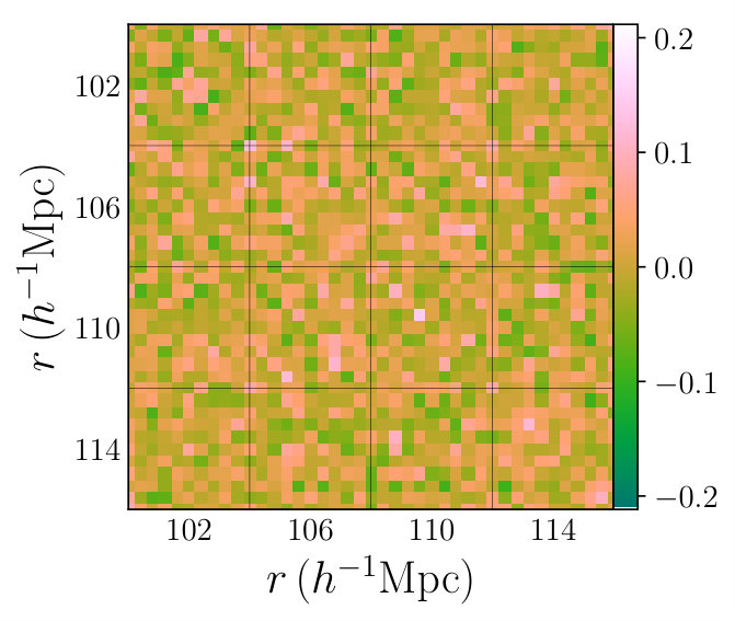 Figure 1
 Figure 2
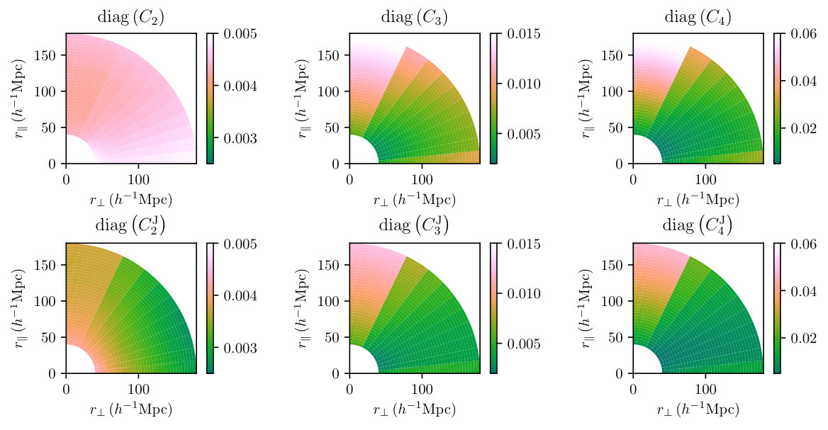 Figure 3
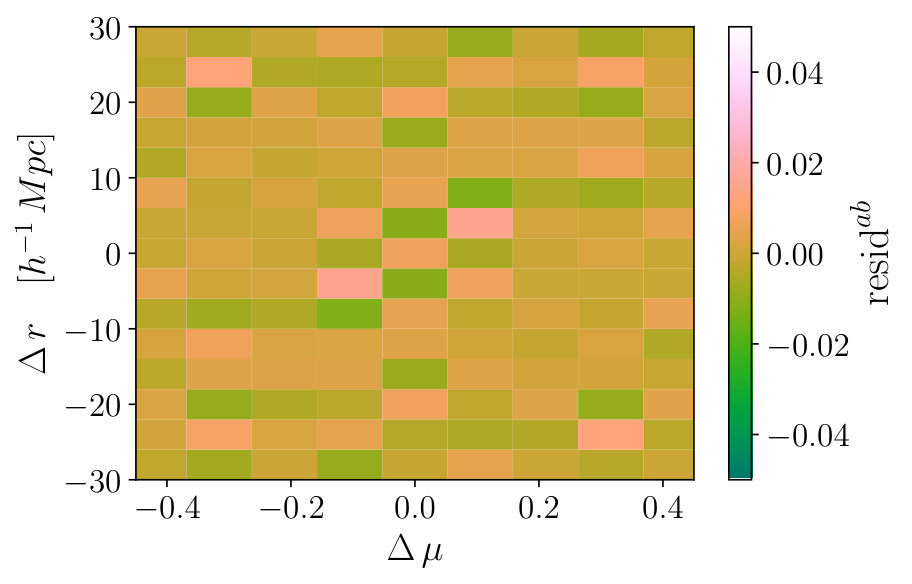 Figure 4
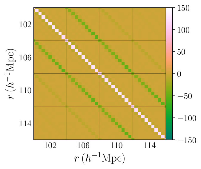 Figure 5
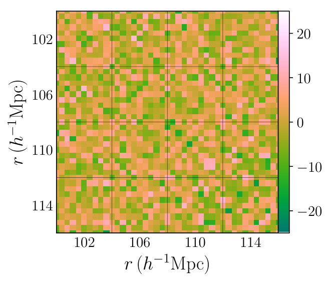 Figure 6
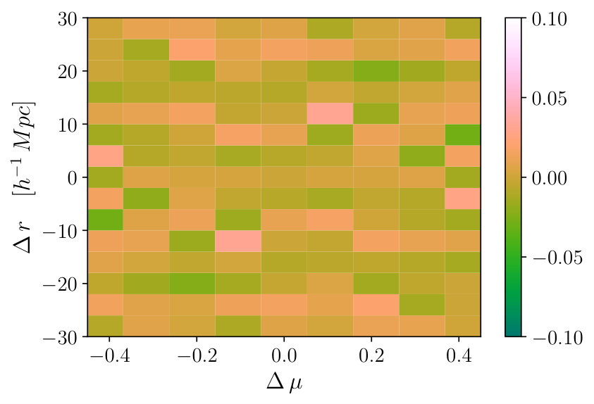 Figure 7
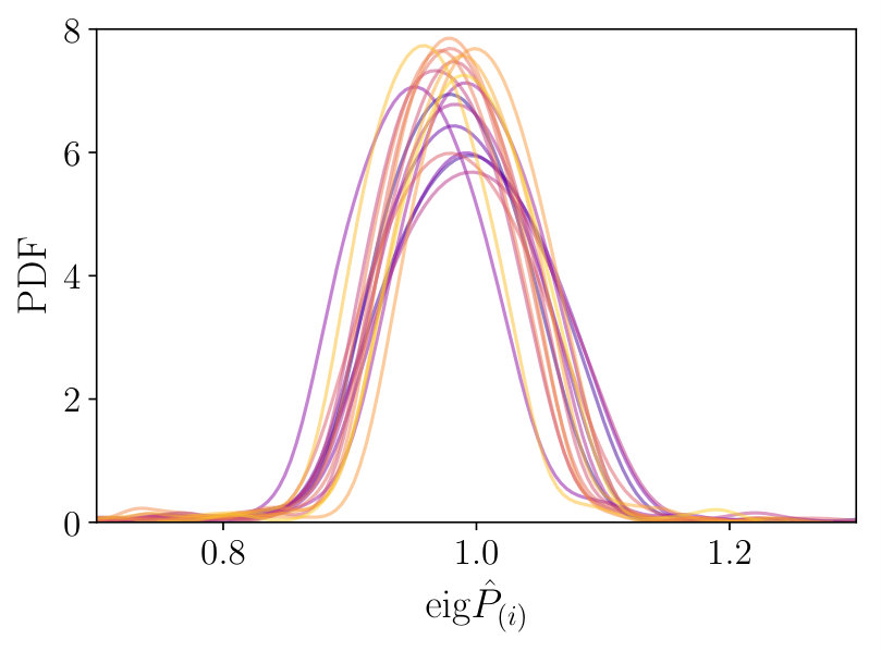 Figure 8
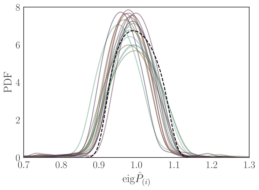 Figure 9
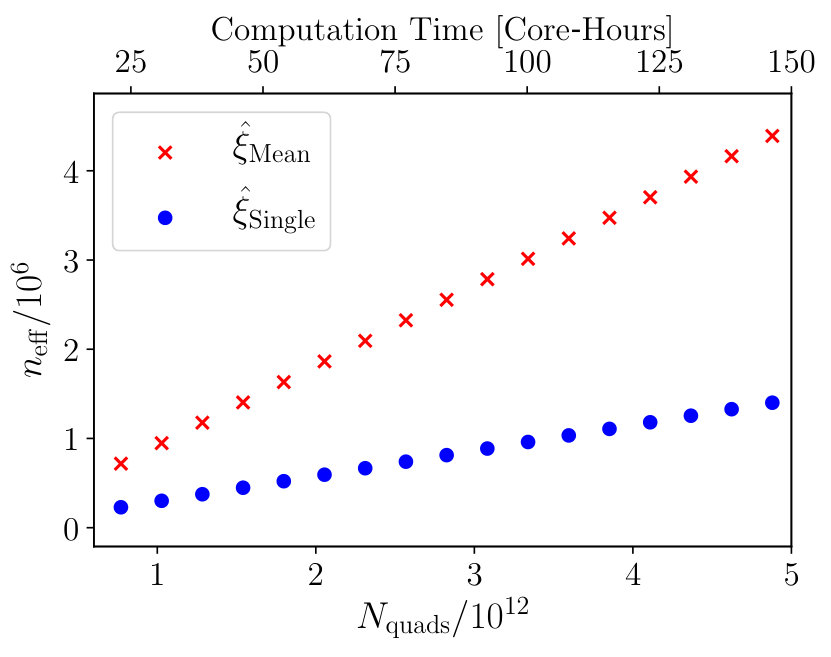 Figure 10
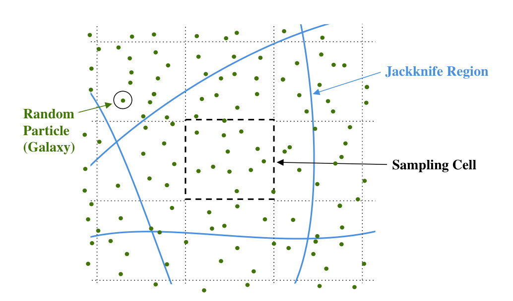 Figure 11
| Fields | Submatrices | |||||
|---|---|---|---|---|---|---|
| 4-point | 3-point | 2-point | ||||
| S | S | S | S | SS,SS | S,SS | SS |
| S | T | S | S | ST,SS | T,SS | ST |
| S | T | T | S | ST,TS | T,ST | (ST) |
| S | T | S | T | ST,ST | (T,SS) | (ST) |
| S | S | T | T | SS,TT | S,ST | (SS) |
| T | S | T | T | TS,TT | S,TT | (ST) |
| T | T | T | T | TT,TT | T,TT | TT |
Peer Reviews
No public reviews on file for this paper yet. If you reviewed it on a platform where reviews are public (OpenReview, ICLR, NeurIPS, ICML), you can paste yours below so the community can read it here.
Code & Models
Videos
No videos yet. Explain this paper in a talk, walkthrough, or lecture? Add one.
RascalC: A Jackknife Approach to Estimating Single and Multi-Tracer Galaxy Covariance Matrices
Oliver H. E. Philcox,1 Daniel J. Eisenstein,1 Ross O’Connell2 and Alexander Wiegand3
1Center for Astrophysics | Harvard & Smithsonian, 60 Garden St., MA 02138, USA
2McWilliams Center for Cosmology, Carnegie Mellon University, Pittsburgh, PA 15213, USA
3Max-Planck-Institut für Astrophysik, Karl-Schwarzschild-Str. 1, D-85741 Garching, Germany E-mail: [email protected]
(Accepted XXX. Received YYY; in original form ZZZ)
Abstract
To make use of clustering statistics from large cosmological surveys, accurate and precise covariance matrices are needed. We present a new code to estimate large scale galaxy two-point correlation function (2PCF) covariances in arbitrary survey geometries that, due to new sampling techniques, runs times faster than previous codes, computing finely-binned covariance matrices with negligible noise in less than 100 CPU-hours. As in previous works, non-Gaussianity is approximated via a small rescaling of shot-noise in the theoretical model, calibrated by comparing jackknife survey covariances to an associated jackknife model. The flexible code, RascalC, has been publicly released, and automatically takes care of all necessary pre- and post-processing, requiring only a single input dataset (without a prior 2PCF model). Deviations between large scale model covariances from a mock survey and those from a large suite of mocks are found to be be indistinguishable from noise. In addition, the choice of input mock are shown to be irrelevant for desired noise levels below mocks. Coupled with its generalization to multi-tracer data-sets, this shows the algorithm to be an excellent tool for analysis, reducing the need for large numbers of mock simulations to be computed.
keywords:
methods: statistical, numerical – Cosmology: large-scale structure of Universe, theory – galaxies: statistics
††pubyear: 2019††pagerange: RascalC: A Jackknife Approach to Estimating Single and Multi-Tracer Galaxy Covariance Matrices–D
1 Introduction
With the next generation of cosmological surveys fast approaching, it is of paramount importance to develop formalisms for creating data covariance matrices to estimate uncertainties on derived cosmological parameters. Future surveys will allow unprecedented exploration of cosmic structure formation and Baryonic Acoustic Oscillations (BAO), through upcoming projects such as Euclid (Laureijs et al., 2011), DESI (Levi et al., 2013) and WFIRST (Doré et al., 2018). With accurate knowledge of experimental covariances, we will additionally be able to perform analysis using cross-correlations of data from different tracer galaxies or surveys.
Conventionally, covariance matrices are obtained from a large suite of ‘mock’ catalogs, simulating large cosmological surveys. Derived two-point correlation functions (2PCFs) for each mock are then combined to estimate the survey covariance. For mocks to be a useful predictor of covariances, we require them to be (a) accurate, such that there is limited bias in the (two- and higher-point) correlation functions and covariance estimates, and (b) numerous, to drive down the noise levels in the computed matrices, degrading final parameter estimates (Dawson et al., 2013; Taylor & Joachimi, 2014; Percival et al., 2014). This clearly requires substantial computational power, thus we should look to approximate methods to obtain such covariances in a fraction of the time. In this paper, we build upon the techniques of O’Connell et al. (2016) and O’Connell & Eisenstein (2019), providing a new algorithm to estimate galaxy covariance matrices from only a single survey in a fraction of the previous computational time. In addition, we extend the formalism to compute covariance matrices between multiple galaxy tracer populations.
Numerous works have demonstrated the effects of noise in the covariance matrix (e.g. Taylor et al., 2013; Dawson et al., 2013; Percival et al., 2014), showing that noise inflates the width of parameter constraints relative to an ideal measurement by for a 2PCF estimated in using . As survey depth increases, so does the number of 2PCF bins, , particularly with the emerging trend of tomographic analysis in current and future surveys (e.g. DES; Abbott et al. 2018, eBOSS; Zhao et al. 2019 and, for weak lensing analyses, KiDS; Hildebrandt et al. 2017). To obtain the same level of precision in our covariance matrices we hence need more numerous and accurate mocks, leading to a steady increase in computational power required. Since such resources are still in limited supply, it is desirable to search for alternative solutions, in particular approximate methods for covariance matrix generation This is usually achieved via covariance matrix modeling (e.g. Pearson & Samushia, 2016; Grieb et al., 2016; O’Connell et al., 2016; Lippich et al., 2019), numerical techniques (e.g. Paz & Sánchez, 2015; Joachimi, 2017) or hybrid approaches (e.g. Friedrich & Eifler, 2018), and allows for low-noise covariance matrices to be computed using far fewer mocks than canonical approaches (see Lippich et al. (2019) for a comparison of such methods).
Approximations of the purely Gaussian covariances are provided by Grieb et al. (2016) and Li et al. (2019), where the former is limited to uniform cubic surveys (and hence is not representative of observational data) yet the latter gives an analytic formalism for computing the 2PCF covariance for an arbitrary survey geometry (building upon the work of Crocce et al. (2011) for the angular 2PCF). Eifler et al. (2014) and Pearson & Samushia (2016) extend this to include non-Gaussianity, with the latter work using a seven-parameter model of the survey-dependent power spectrum covariance that can be calibrated with (a small number of) simulations. Similarly, in O’Connell et al. (2016), it was shown that, for a single set of tracer galaxies, a configuration-space covariance matrix can be well represented by a theoretical approximation computed solely from 2PCFs, given knowledge of the survey geometry and weight functions. Non-Gaussianity was found to be incorporated effectively by a simple rescaling of the galactic shot-noise, again calibrated via a small number of mock galaxy catalogs. This produced covariance matrix estimates of comparable precision using far fewer mocks than purely mock-based approaches.
In this paper we will use the shot-noise rescaling introduced in O’Connell et al. (2016) to model non-Gaussian contributions to the covariance matrix. The physical intuition behind this is as follows. Non-Gaussian covariance matrix terms are sourced by higher-point correlation functions, which primarily describe additional clustering on small scales (usually less than the binning width). By enhancing the shot-noise, we increase the clustering power on infinitely small scales, which is found to be a good approximation in practice. Mathematically, this is equivalent to replacing integrals over the higher-point correlation functions with their contractions (which are simply shot-noise terms); a fair assumption if the functions are dominated by their squeezed limits on the relevant scales. Additional motivation comes from parallels with Effective Field Theory, with higher order corrections being absorbed into a ‘renormalized’ shot-noise parameter. Whilst this cannot significantly modify clustering at large galaxy separations, this is not found to be an issue since the galaxy field appears to be highly Gaussian on these scales. In Vargas-Magaña et al. (2018), the validity of this approach was clearly demonstrated in its application to BAO parameter constraints, although we expect the approximation to work less well on smaller scales, such as for quasi-linear redshift-space distortions.
A number of recent papers have considered the determination of 2PCF covariance matrices from only small volumes (e.g. Howlett & Percival (2017), Klypin & Prada (2018) and, for super-sample covariance, Barreira et al. (2018)), showing this to be a viable approach to constraining larger scale covariance matrices. This was further developed in O’Connell & Eisenstein (2019), where the technique of constraining the shot-noise rescaling directly from the data was introduced, splitting the data into small jackknife regions and computing the 2PCFs in each. Given these estimates, a jackknife covariance matrix was obtained, which was compared to a theoretical prediction in order to compute the shot-noise rescaling. This approach thus allows covariance matrices to be estimated purely from data, without calibration with mocks, and additionally allows us to use any input survey geometry.
In this paper, we introduce an improved sampling algorithm, which is able to produce low-noise estimates of the covariance matrix in a fraction of the previous computation time. We adopt a similar jackknife-calibrated rescaling approach to O’Connell & Eisenstein (2019), yet switch to the unrestricted jackknife formalism, which allows for more precise determinations of rescaling parameter. Covariance matrix computation is greatly expedited by a new grid-based importance sampling technique, drawing sampling points from random galaxy position catalogs (such as those used for pair counts) rather than newly generating them from some mask and number density distribution. The updated sampling allows the code to run times faster than previous codes (O’Connell et al., 2016) with no loss of accuracy.
With new data releases from galaxy surveys such as the Extended Baryon Oscillation Spectroscopic Survey (eBOSS; Dawson et al., 2016), we will soon be able to obtain improved constraints on large scale structure parameters by using multiple galaxy tracers, for example the Emission Line Galaxies (ELG) and Luminous Red Galaxies (LRG) populations. For such analyses, we require cross-covariance matrices, evaluating the associations between auto- and cross-correlation functions. The addition of such complexity conventionally requires more mocks to be computed; yet via our approach, arbitrary cross-covariances can be computed with ease. We describe an extended formalism to compute these matrices from data alone, with all possible two-tracer covariance matrices requiring only times the computation time of a single tracer survey.
The full analysis pipeline for this fast and flexible approach has been condensed into a publicly available C++ and Python package; RascalC111https://github.com/oliverphilcox/RascalC with extensive documentation showing its usage for single- and multiple-tracer cosmology.222https://RascalC.readthedocs.io Included are all relevant routines allowing estimation of a set of covariance matrices simply from input survey or random galaxy position files in sky or Cartesian coordinates. The flexibility of the code ensures that it can be simply altered to take more complex forms for the theoretical covariance matrix, for example with some estimation of the 3- or 4-point correlation functions, or a different jackknife formalism. The authors are happy to assist with this process on request.
The structure of this paper is as follows. In Sec. 2 we present the theoretical covariance matrices for the new unrestricted jackknife formalism, with their evaluation discussed in Sec. 3, which outlines our new (and highly efficient) sampling scheme. Sec. 4 gives a description of the computational algorithm used here, followed by a comparison to previous code and an application to simulated Quick Particle Mesh (QPM; White et al., 2014) data in Sec. 5. The approach is generalized to deal with multiple galaxy tracer populations in Sec. 6 before we finish with conclusions and mathematical derivations in Sec. 7 and appendices A-D.
2 Theoretical Covariance Matrix Estimators
We begin by considering the covariance matrix estimators used in this paper. For clarity, we first recapitulate the full covariance matrix integrals given in O’Connell et al. (2016) before discussing the modification to jackknife covariance matrices. Throughout this section, we assume space to be discretized into a set of small cells (each of which can contain at most one galaxy) to simplify our expressions. As in O’Connell et al. (2016) and O’Connell & Eisenstein (2019) the indices refer to these cells and not the galaxies found therein.
2.1 Full Covariance Matrices
The standard estimator for the anisotropic 2PCF is given by
[TABLE]
(Landy & Szalay, 1993), summing over all pairs of cells (denoted and ) and using the definitions
[TABLE]
where and are the mean number density and weight in cell and is a binning function (which is unity if the pair of cells lies in the bin and zero else). Here, the observed galaxy density is , such that , and the weights are set by the utilized survey, e.g. FKP weights (Feldman et al., 1994) in mock catalogs for the Baryon Oscillation Spectroscopic Survey (BOSS; Alam et al., 2015, 2017). From we may construct the covariance matrix via
[TABLE]
In O’Connell et al. (2016) it was shown that, by expanding the summation into 2-, 3- and 4-point terms and using Wick’s theorem to expand factors, this leads to the full survey theoretical covariance estimator in bins
[TABLE]
with components defined by
[TABLE]
Here, we denote the 2PCF by (for cell centers at and ) and the three- (four-)point correlation function by (). Note that we have exploited the relabelling symmetry of the 3-point matrix to exchange and with respect to O’Connell et al. (2016, Eq. 2.25); this is done for later efficiency. These may be alternatively written in continuous space via the replacements , and .
An important assumption in this paper (and in previous works) is that non-Gaussianity can be well approximated by simply rescaling the level of shot-noise in the survey by a factor ,333For clarity, we denote the shot-noise parameter as rather than the previously-used . as justified in the introduction. This can be calibrated either by jackknives or mock data, and allows us to drop the higher point correlation functions and in the above expressions giving the new estimator
[TABLE]
2.2 Jackknife Covariance Matrices
2.2.1 The Unrestricted Jackknife Formalism
One of the key benefits of a large cosmological survey is the ability to split the survey into sub-regions to produce multiple estimates of quantities such galaxy correlation functions. A standard approach to this is to use jackknives, where we split the survey into regions (as depicted in Fig. 1), and compute an estimate of the 2PCF with each region left out in turn (e.g. Norberg et al., 2009; Friedrich et al., 2016). In this work, the jackknife covariance matrices are not used as estimates of the full-volume covariance matrix, but rather to constrain the shot-noise rescaling parameter . This is done by comparing theoretical and data-derived jackknife covariance matrices, and the optimal is then passed to the full covariance estimator (Eq. 2.6), giving an estimate of the (non-Gaussian) complete survey covariance.
As noted in O’Connell & Eisenstein (2019), cosmological jackknives suffer from additional complexities not found in traditional jackknife approaches, most notably that different jackknife regions are not independent and pairs of cells (containing galaxy positions from the random or survey catalogs) can straddle jackknife regions, which is important for 2PCF analyses, where we are primarily interested in pair counting. There exist several choices of jackknife formalism corresponding to different weightings between cells (or particles in the continuous limit), denoted for cells and and jackknife region . For the restricted jackknife, as used in O’Connell & Eisenstein (2019), we assign unit weight to pairs of cells that both lie in region and zero weight else, giving , where is unity if is in region and zero else. In this paper, we instead adopt the unrestricted jackknife formalism, which includes cell pairs which straddle the jackknife region. We assign half-weight to cell pairs where only one cell is in the region and unit weight to pairs which are both in the same region, giving the modified form
[TABLE]
This allows us to include all cell pairs and to probe the 2PCF on scales larger than the jackknife region. Whilst these jackknifes are by no means independent, this is not an issue in our analysis because the jackknife covariance is not being used to estimate the full-volume covariance directly. (This avoids having to introduce additional complexities such as the ‘pair jackknife’ of Friedrich et al. (2016), which assigns half of all particle pairs crossing a given jackknife region to the first region and half to the second to remove bias.) Since pair counts are by nature additive, it is true here that the covariance matrix of jackknife correlation functions can be rewritten as a rescaled version of the sample covariance between the estimates of the 2PCF in each jackknife region (rather than those excluding each region). This simplifies the analysis greatly, and hereafter we will only consider estimates of within each region.
2.2.2 Correlation Function Estimators
In a jackknife region , the 2PCF may be estimated as a sum over fine cells, , , in an analogous fashion to Eq. 2.1:
[TABLE]
for arbitrary jackknife weighting function . From these, an overall estimate is defined via
[TABLE]
where . The weights, , are analogous to the volume fraction of each region, but allow for variations between 2PCF bins. Utilizing the definitions of Eq. 2.8, this becomes
[TABLE]
for . For the unrestricted jackknife, where , and reduce to and ; the full survey forms (cf. Eq. 2.1).
2.2.3 Covariance Matrix Integrals
As in O’Connell & Eisenstein (2019), we can compute the weighted jackknife covariance matrix (in bins ) from the jackknife 2PCFs as
[TABLE]
which can be used both to construct a theoretical model of the covariance matrix and to find an estimate directly from data, using estimates from exhaustive pair counting. The weighting function is here set equal to the 2PCF weighting .444The exact choice of is not important here, since we attempt only to fit a theoretical estimate of to one constructed from data.
Since each unrestricted jackknife uses all particles in the survey, we expect non-negligible correlations between individual estimates (expected to be negative for a uniform survey), meaning that they are not strictly independent. This implies that the jackknife covariance matrix is not a good estimator of the full-survey covariance, and is likely to be an underestimate on average. In our context, the jackknife covariance matrix is being used solely to fit for the shot-noise rescaling parameter , rather than estimate the full-survey covariance and, since this effect is common to both theory and data estimates, it may be ignored.
Eq. 2.11 may be expanded analogously to the full covariance matrix estimator, and a full derivation is presented in Appendix A. As before, we assume a shot-noise rescaling parameter and expand the summations and random field expectations to yield the estimator555It is not obvious a priori that the jackknife covariance will have the same shot-noise rescaling parameter as the full-covariance matrix, as the two matrices are different in expectation. In O’Connell & Eisenstein (2019), the approach was tested using the restricted jackknife formalism and estimates of from jackknifes were found to agree with those from mocks at high precision.
[TABLE]
where we define
[TABLE]
(including the non-Gaussian terms for generality, although these are not used in the computation). The weighting tensor is given by
[TABLE]
and, in the case of the unrestricted jackknife, simplifies to
[TABLE]
via Eq. 2.7, where we define as the jackknife region of cell . Equivalent expressions for the jackknife covariance matrix terms in continuous space are given in Eqs. A in the appendix. The theoretical jackknife covariance model defined by Eqs. 2.13 will later be fit to the sample jackknife covariance of Eq. 2.11 (using measured 2PCF estimates in each jackknife) to constrain the shot-noise rescaling parameter .
We note significant differences between the forms of O’Connell & Eisenstein (2019) and those here. In the former, the jackknife covariance was taken as ; we instead use the full jackknife covariance of Eq. 2.11 for better comparison with observational data, which gives a different prefactor, an additional term (cf. Sec. 2.2.4) and new weighting tensors.
2.2.4 The Disconnected Term
In the expectation of the integral, we note the presence of a disconnected 4-point term involving which may be factored into a product of 2-point terms, summed over the jackknife region . This was not present in O’Connell & Eisenstein (2019) and arises due to the different form of the jackknife covariance matrix adopted. Returning to the summation form of the integrals, we may rewrite this term (hereafter denoted ) in the following separable form:666Note that we switch from summations to a pair of and summations here. Whilst this generates two additional lower-point terms, both involve an additional factor of in the integrand (unlike for the contractions in the main integrals), giving negligible contributions to: the integrated term.
[TABLE]
where we define
[TABLE]
analogously to . In realistic surveys, the disconnected term is expected to be small, and the conditions under which it cancels entirely are discussed in appendix B.
3 Evaluation of the Covariance Matrix Integrals
Computation of the covariance matrix integrals derived above (Eqs. 2.5 and 2.13) allows us to compute a useful full-volume model covariance matrix. To evaluate these terms, we will make use of a new sampling strategy, which is described below. This divides up the survey into ‘sampling cells’ (formalized in Sec. 3.1) and uses Monte Carlo importance sampling methods to pick these in an efficient manner, giving an algorithm that is faster than previous codes (O’Connell et al., 2016) by a substantial factor ().
3.1 The Sampling Grid Formalism
To efficiently compute the high-dimensional integrals in Eqs. 2.5 & 2.13, we require Monte Carlo sampling methods, where we draw sets of points in three-dimensional survey space (hereafter ‘pairs’, ‘triples’ and ‘quads’) and use these to evaluate the -dimensional integrals via summation of the integrands (see Kilbinger & Schneider (2004) and Joachimi et al. (2008) for an application of similar ideas to cosmic shear covariance in configuration- and Fourier-space respectively). In previous work (O’Connell et al., 2016; O’Connell & Eisenstein, 2019) using the Rascal code,777https://github.com/rcoconnell/Rascal random sampling positions were generated from the survey geometry defined by the experiment mask and an estimate of the redshift-dependent number density and particle weight . Here, we adopt a new approach, making no use explicit use of the mask, but instead using catalogs of ‘randoms’ provided by galaxy surveys, consisting of random galaxy positions (denoted ‘random particles’) distributed according to the survey selection function. These are primarily used to compute counts for 2PCF computations. Their number densities, are expected to have the same mean spatial dependence as for the survey galaxy distribution, ,888When this approach is applied to the jackknives, there is an implicit assumption that the galaxy-to-random-particle ratio is constant between jackknives. Our formalism could be generalized to account for this, but, since jackknives are used only for calibration, the problem can be avoided by fixing the jackknife pair counts normalization to the full-survey value, as in Sec. 3.5. and we assume the distribution of random particle weights matches that of the galaxies.999It may seem tempting to include the weights in the normalization to allow for differences between and ; this is not helpful in this context, since the 2- and 3-point integrals differ in the number of and factors. We may thus write
[TABLE]
for a total of and galaxies and random particles respectively.
For computational efficiency, these random particles are placed on a cuboidal sampling grid encompassing the entire survey region, partitioning them into a number of cubic sampling cells, each of which contains a small number particles, as illustrated in Fig. 1. (These cells are distinct from the small regions used to define the discrete summations in Sec. 2 which contained at most one particle.) This sampling grid-based approach allows for fast and trivially parallelizable code, where we can pre-assign probabilities of picking each sampling cell according to some given sampling strategy, ensuring that all elements of the covariance matrices are well sampled. In this approach, there is no explicit dependence on a survey mask which is useful since (a) future surveys may only generate random particles rather than a mask lookup function and (b) there is a large computational efficiency boost, as sampling reduces to picking random sampling cells, without having to query a complex mask.
3.2 Importance Sampling Techniques
To evaluate high-dimensional integrals, Monte Carlo techniques are required, in particular importance sampling, where we pick points in parameter-space in such a way as to allow for fast convergence of the integral. To see how this may be applied in practice, first consider the integral of an arbitrary function of a single (3D) spatial coordinate over the survey;
[TABLE]
where is some normalized weighting function satisfying . Treating as a probability density function (PDF) for , this may be rewritten as an expectation over , , which can be sampled by drawing random positions according to the PDF ;
[TABLE]
where we make a total of from (the approximation becomes exact in the limit ). Importance sampling tells us that we may also draw points from a different PDF, , by writing
[TABLE]
where the expectation is now over and positions are sampled from this PDF, with a reweighting by . Whilst this may not seem useful, it allows us to manually choose the sampling distribution and alter the estimator’s efficiency. The optimal function is found by minimizing the variance of the estimator for ; this can be shown to be proportional to . In practice, we cannot sample directly from , thus we instead choose some which is (a) easy to sample from and (b) similar in form to . This allows us to preferentially sample regions where the summand is large, leading to faster convergence.
In this paper, we are interested in sampling integrals which depend on sets of two, three and four points in space. To demonstrate the extension of the above methodology to higher dimensional cases, we consider a two-point case; the integral of a function weighted by the product of (continuous) galaxy number densities :
[TABLE]
converting to random particle densities via Eq. 3.1. In this case, the normalized PDF for drawing a pair of (ordered) points at and is
[TABLE]
which allows us to rewrite the integral as an expectation over and hence a sum (as for the 1-point case above);
[TABLE]
for , where we draw a total of sampling points. Notably, in the above integral and estimator, there is no inclusion of or since we are drawing points from a distribution which matches that of the galaxies (unlike in O’Connell et al. 2016 and O’Connell & Eisenstein 2019). As before, this may be recast into an expectation over some different PDF via
[TABLE]
In our context, instead of choosing random pairs of positions from the survey geometry defined by some mask, we simply pick pairs of particles from the set of all possible pairs of input random galaxies (with total pairs). Henceforth, we will use the roman indices , , etc. to label such particles. This implies that we must switch to discrete statistics, and the aforementioned PDF (Eq. 3.6) is transformed into a uniform probability mass function (PMF) (as we draw two ordered particles and uniformly from the set of particles). now becomes the PMF for drawing two points from the set of random particles, with some user-defined weighting. Thus, inserting the forms of the PMF, the general 2-point integral becomes
[TABLE]
where we draw particles according to the PMF . This extends naturally to summations of triples and quads of particles, using the appropriate normalization by the number of samples and for the -point integral.
3.3 Sampling Cell Selection & Integral Estimators
3.3.1 Cell-Based Stochastic Estimators
It remains to decide how to choose sets of particles (denoted ) to sample, and hence the PMF, , for the -point integral. In our implementation, this is assisted by the use of the aforementioned sampling grid cells (denoted , , , ). Given some initial particle in sampling cell , subsequent particles are chosen by first picking a sampling cell via some PMF (depending only on the relative distances between and ) and choosing one of the particles, , inside at random (from a total of particles in ). For pairs of random particles , we obtain a distribution function , depending only on the occupation and separation of sampling cells and . For normalization, we include a prefactor , which corresponds to the number of possible choices of the particle. The final form of the general pair estimator for samples is thus
[TABLE]
which again naturally extends to higher order integrals, e.g. sampling from the probability distribution for the 4-point term. Notably, the particle-selection PMFs are reduced to simply probability distributions over sampling cell positions, which can be pre-computed efficiently. Using this approach, estimators for the jackknife covariance matrix integrals (Eqs. 2.13, assuming Gaussianity) become
[TABLE]
where the summations run over individual random particle positions. (See Sec. 3.3.3 for the disconnected term estimator). This gives the correct normalization factors to be included in the summation, and extends naturally to the full (non-jackknife) integrals with the omission of the prefactor, the disconnected term and tensors. The term may be estimated stochastically as
[TABLE]
Since the jackknife weights depend on (through ) these must be computed separately before we estimate the full integrals. As this only depends on pairs of points, little additional computational expense is required, making it feasible to compute this by counting all possible pairs without importance sampling (see Sec. 4.1). This gives the functional form
[TABLE]
where , run over all random particles. The term can simply be found via in the unrestricted jackknife formalism (and can be compared to the above stochastic result as a useful test).
3.3.2 Sampling Cell Selection Probabilities
The choice of the probabilities (giving the likelihood of selecting sampling cell containing particle from initial sampling cell ) allow us to optimize the performance of the Monte Carlo estimators. We choose the probability for selecting a secondary cell at separation from a primary cell to be proportional to
[TABLE]
where is the value, at spatial position , of a cubic sampling grid cell window function centered on position of width . Here is the kernel function, which is here integrated over both sampling grid cells.
Although the sampling cells are cubic, we may obtain much more tractable solutions to Eq. 3.14 by treating them as spherical (keeping the volume fixed). In addition, by making the approximation that the window functions are spherical Gaussians rather than top-hat functions, the integral can be transformed to
[TABLE]
also assuming to be a function of only. Note that importance sampling just requires the sampling distribution to be known, not to be perfect, thus these approximations do not compromise on accuracy (and lead to only a tiny reduction in efficiency). This is shown in appendix C and can be computed numerically for arbitrary kernel functions.
In this paper, we will use two forms for the kernel function; and , used for efficient importance sampling and uniform filling of all covariance matrix bins respectively (see Sec. 4.2). With the latter kernel, we have the semi-analytic result (derived in appendix C)
[TABLE]
for Dawson-F function (Dawson, 1897) (which can also be written in terms of confluent hypergeometric functions). This tends to at large radius but avoids infinities at small . It is pertinent to note that simplifications in the form of the kernel and window function do not bias the computed covariance matrices, but just change the sampling strategy slightly. It is thus desirable to have a simple expression for . These forms set the probabilities used in the importance sampling estimator summations (e.g. Eqs. 3.11), which are computed before any Monte Carlo integration is performed.
In order to use the kernel, we require that the input (radial) 2PCF is strictly positive over the full binning range, else some sampling cells will be erroneously excluded from the analysis. To ensure this we use the modified kernel
[TABLE]
which was found to give efficient sampling of all sampling cells in the required range.
3.3.3 Disconnected Term Evaluation
The disconnected part of (cf. Sec. 2.2.4) is estimated in a different manner to the rest of the 4-point integral. For an arbitrary quad of points , the and separations are constrained by the choice of bin (via the and functions), but the and separations are ab initio unconstrained. If these are large, we will obtain a vanishingly small contribution to the connected 4-point terms since for large . However is independent of and , making its evaluation more complex.
As shown in appendix B, the term should be small, yet the form of implies that this cancellation occurs via the balance of large positive contributions at small and separations with many small negative contributions on large scales (when and belong to different jackknife regions). Computationally, this only works if we consider the full range of and separations, yet we usually impose a cut-off at some large separation ( Mpc/h) for efficiency.
To ameliorate this, we use the alternative form of (Eq. 2.2.4), which is computed from 2-point quantities (), which are generally known to higher precision than the 4-point terms. Due to the finite sampling strategies used in computation of the terms, we still expect Poissonian fluctuations in the estimated values of , which reduce in amplitude as we evaluate the function at more points. For off-diagonal terms, this will lead to the estimate fluctuating about zero, yet for the leading diagonal (where ), we will not get cancellation, since the term involves a sum over which is strictly positive. This can be removed by using two disjoint sets of survey points to compute and . This modifies the disconnected to the form
[TABLE]
Here the labels (1) and (2) refer to estimates derived from different sets of random particles. The Poissonian fluctuations between the two estimates are thus uncorrelated, removing the spurious diagonal term on average. We note that we must also compute for each set of particles individually to avoid obtaining substantial negative correlations between the two factors (as a large in one set of random particles would otherwise encourage a small in the other if were computed from all particle pairs including both random subsets). The weights (for ) are computed stochastically for the disconnected term, along with . This is unlike that used for the rest of the analysis, but is appropriate since the 2-point terms are generally well-known and we expect the overall disconnected term to be small.
In practice, we assign each random particle to either subset 1 or 2 on initialization and computing contributions to the relevant count if both particles lie in the relevant bin and discarding else. This gives the estimator form for and :
[TABLE]
where the superscripts refer to the relevant values for the -th set of random particles. In addition, it is a fair assumption to assume as . In all tests, this term has been found to be small (several orders of magnitude smaller than the dominant terms) but may be important for some particular choices of geometry and/or jackknife regions.
3.3.4 Monte Carlo Estimator Scalings
It is pertinent to consider the dominant scalings of the above importance sampling integral estimators. These are as follows:
Number of random points, : Rescaling , we expect the number of particles in each sampling cell to increase by a factor on average, thus . From Eqs. 3.11 & 3.12, it is clear that and the covariance matrix estimators ( and ) are invariant to this rescaling, which is as expected, since the random points are solely a computational aide. 2. 2.
Number of galaxies, : Rescaling has no effect on random particle terms, sampling cell probabilities or (which is computed via normalized pair counts). Thus and (and similarly for the jackknife Monte Carlo estimators). Changing the number of galaxies in the survey volume thus reweights the relative contribution of the 2-, 3- and 4-point integral terms. 3. 3.
Average particle weight : Rescaling for all particles implies since we expect the random particle weight distributions to match that of the galaxies. Since all covariance matrix estimators involve four factors of in the numerator, and involves two factors of , we expect any dependence of the estimator on to vanish. 4. 4.
Number of jackknife regions, : Since (for the unrestricted jackknife) is independent of , we must have (as there are terms in total), and thus . Inspection of the expansion of (Eq. 2.15), shows that this also scales as . In the jackknife integrals, the prefactor scales approximately as , thus at leading order (which is exact if all jackknife regions are identical).
3.4 Shot-Noise Rescaling & Precision Matrices
Given the Monte Carlo covariance matrix estimators, it remains to compute the optimal shot-noise rescaling parameter , which approximates non-Gaussianity in the model. Following O’Connell et al. (2016), we do this by maximizing a likelihood based on the Kullback-Leibler (KL) divergence (Kullback & Leibler, 1951) between our estimate of the jackknife covariance matrix, , and the data-derived estimate, , which uses the 2PCF estimates from only a single dataset, without reference to mocks. Denoting the theoretical precision matrix as (equal to the inverted matrix in the noiseless case), we formulate the likelihood as
[TABLE]
for a total of bins.101010We use the likelihood here rather than (with , since the latter requires inversion of the singular jackknife data covariance matrix. It is pertinent to note that this likelihood does not account for noise in the fitting matrices, which can cause a small bias, as will be discussed in future work. Here, is determined by maximizing numerically, which requires
[TABLE]
utilizing the identities
[TABLE]
As shown in O’Connell & Eisenstein (2019), a simple inversion of a noisy covariance matrix yields a biased estimate of the precision matrix . For a general (covariance) matrix , a bias-corrected estimator of is given by
[TABLE]
computed using independent estimates of the matrices, denoted , with indicating the mean of the other samples, excluding . This requires multiple model covariance matrix estimates, which are easy to obtain using our stochastic sampling algorithm (Sec. 4. This is used to compute the full and jackknife precision matrices here, free from quadratic bias.
For a matrix following Wishart statistics, computed from samples in , we have the general result (Wishart 1928; see also Hartlap et al. 2007 for application to cosmology);
[TABLE]
Comparison with Eq. 3.23 allows us to define the effective number of mocks, for a general matrix, which would be equal to in the case of Wishart noise. Using the mean determinant per mode as a proxy for ;
[TABLE]
This differs from the definition of O’Connell et al. (2016); O’Connell & Eisenstein (2019), which uses the variance of for off-diagonal elements, and is chosen to avoid the former ambiguities in the choice of bin. Here this is performed for and in post-processing to assess the precision of the computed matrices.
3.5 Correlation Function Estimation
A key input to the covariance matrix integrals is the estimated 2PCF for and angular coordinate , where is the angle of a pair of galaxies from (a) their mean line of sight position (for a non-periodic dataset) or (b) the axis (for a periodic simulation). In addition, we require estimates of the 2PCF in each jackknife region, in order to compute the data jackknife covariance matrix which can be compared to theory to estimate the shot-noise rescaling . To compute from a data-set, we use the Landy & Szalay (1993) estimator, which defines a full-survey 2PCF in bin as
[TABLE]
where , and represent normalized auto- and cross-pair counts for the galaxy and random particle fields. These are defined as
[TABLE]
for , weighting by the product weight and summing over all particles in each field. The normalization accounts for differences in number of particles in each dataset. For the unrestricted jackknife correlations, the estimator is modified to
[TABLE]
where the jackknife pair counts are defined as
[TABLE]
These estimates are then used to compute the data jackknife covariance matrix via Eq. 2.11. Notably, we normalize the jackknife pair counts by the same factors as for the full-survey pair counts, not the summed weights of the relevant jackknife regions. This means that our estimates are not truly representative of the 2PCF in the unrestricted jackknife , with discrepancies arising since we ignore differences in the ratio of galaxies to random particles between different jackknives (which occur both due to the small number statistics and large scale correlations). Here, this form is preferred since it can be simply compared against our theoretical jackknife estimate, , which assumed a uniform galaxy-to-random ratio for each jackknife.
Using the Landy-Szalay 2PCF estimators above, we obtain averaged across radial and angular bins. For out covariance matrix estimators (Eqs.2.5 & 2.13), we instead require knowledge of at arbitrary radii and angles, thus we must convert from a binned to a continuous function. A simple solution would be to use the bin-averaged estimates as the values of at the bin-centers (denoted and ) and use linear interpolation to convert this into continuous space. However, this introduces a non-negligible bias, since the true values of are not equal to . In this paper, as in O’Connell et al. (Sec. 3.2 2016), we adopt a different approach, computing a corrected set of 2PCF values, . A continuous function is computed from these via linear interpolation which, by construction, reproduces the binned values when averaged over the original bins.
To compute , we adopt an iterative procedure, gradually refining the estimates of the 2PCF values at the bin centers. Given a continuous function from estimates, , the bin-averaged 2PCF is given by
[TABLE]
These are computed in the same manner as the integrals (described below), with a very small level of noise. This is then compared to the true value (as found via the Landy-Szalay estimator) which is used to find the next estimate as
[TABLE]
Starting from an initial estimate of , we are able to obtain sub-percent agreement between and after iterations.
4 Algorithm Overview
We here review the structure of the RascalC code used to implement the Monte Carlo estimators and perform all necessary pre- and post-processing.111111https://github.com/oliverphilcox/RascalC
4.1 Pair Counting
To evaluate the jackknife covariance integrals (Eqs. 2.13 or A), we require an estimate of the weights to allow computation of the tensor. This in turn requires knowledge of the (and hence functions), which are 6-dimensional integrals, depending on a pair of points in 3-dimensional space. In addition, the functions are an important normalization factor for both full and jackknife covariance matrices. Although these could be computed stochastically (as in Eq. 3.12), it is relatively simple to compute them exhaustively, as a weighted sum over all pairs in each bin obeying the correct unrestricted jackknife criterion.
In practice, these are computed using the corrfunc code121212https://corrfunc.readthedocs.io/en/master/ (Sinha & Garrison, 2017), which efficiently counts all possible pairs of particles in two input fields, given a set of input bins. As in the importance sampling estimators for the 2-, 3- and 4-point matrices (Eqs. 3.11), we must multiply the corrfunc and estimates by a factor to account for the different numbers of galaxies and random points (as in Eq. 3.13).
For the unrestricted jackknife counts in a jackknife region , the jackknife-pair counts is given by a pair count using the cross-correlation of the pairs in the full survey with those in the jackknife region , weighted by the product of particle weights . This has the desired effect of weighting assigning a weight of unity to pairs entirely in the jackknife and half for those with only one-half in the jackknife. This can be done in iterations of corrfunc, and does not require a significant increase in computation time compared to the computation. In addition, we may simply co-add the estimates to find for each bin in this jackknife formalism.
In addition, corrfunc pair counts may be used to define the input full-survey and jackknife 2PCFs (but can be specified separately, if required). This simply uses the Landy-Szalay formalism (Eqs. 3.26 & 3.28), requiring pair counts between data and random-particle fields and . For the estimation, this is done as for , with normalization now given as the summed weights in the two input fields. For jackknife pair counts of two fields , we use the mean pair counts from the entirety of field and the jackknife region of field and from the entirety of field and the jackknife region of survey , if (i.e. for pair counts). We note that the binning used for the functions should match that of the covariance matrices, but may differ from the input .
4.2 RascalC Algorithm Structure
As described in Sec. 3, we compute the covariance matrix estimates by summing over sets of four particles (‘quads’). The basic structure may be summarized as follows.
First, the survey region is discretized into a number of cubic sampling cells, to allow an efficient implementation of the Monte Carlo importance sampling (as described in Sec. 3.1), and random particles are read-in, assigning the -th particle to sampling cell (which can contain than one particle). For later estimation of the disconnected term, each particle is assigned to random subclass 1 or 2 (Sec. 3.3.3).
Given the sampling cell size, the transition probabilities between cell and (Sec. 3.3.2) are computed both using the kernel (Eq. 3.15) and the kernel (Eq. 3.16). Since these depend only on inter-cell separations, they may be precomputed without knowledge of the individual particle positions. Here, numerical integration is performed for the kernel via the cubature C++ package.131313https://github.com/stevengj/cubature, up to a maximum separation corresponding to the cut-off beyond which correlations are set to zero. When using a large enough value for this cut-off, the truncation was found to give no significant impact on the overall result.
At this point, the 2PCF is computed from the input binned function as described in Sec. 3.5, and the bin-averaging integration is performed stochastically, by drawing pairs in the same manner as with the 2-point terms below. This refinement cannot be performed alongside the 2-point integral computation, since is an important part of the covariance matrix integrands.
Following such pre-processing, a stochastic computation of the 2-, 3- and 4-point integrals is performed via the Monte Carlo estimators of Eqs. 3.11. This is done over a number of independent epochs , each of which utilizes each random particle in turn as the primary particle, and may be run on separate cores. By splitting up the computation into shorter epochs, we produce independent estimates of the integrals, allowing better estimation of the precision matrix (cf. Sec. 3.4) and the effective number of samples () in the code to be assessed. In each epoch, we adopt the following procedure (chosen to ensure minimal re-computation of quantities such as the interpolated ):
Iterate over each non-empty cell (denoted ) in the sampling grid. This ensures that every random particle (in a total of cells) is used in each epoch. 2. 2.
Randomly select a second sampling cell () from with probability , using the pre-computed probability grid. This is performed using the Walker-Vose alias method (Walker 1974, 1977; Vose 1991, in the implementation of Joachim Wuttke141414apps.jcns.fz-juelich.de/man/ransampl.html) and selects one realization from a discrete set of possibilities with pre-assigned probabilities, here the grid of neighbouring sampling cells. To draw the cell, we use the kernel (with defined by Eq. 3.16), to ensure that all bins are filled roughly uniformly, truncating at the maximum radial bin size. If the selected cell lies in the survey region and is non-empty, we pick a single particle () from the cell and iterate over all particles in the cell. For each -pair of particles, we do the following;
- •
Compute the correlation bin from the separation of the particles.
- •
Evaluate the correlation function at the particle separation () via linear interpolation of the input 2PCF.
- •
Find the contributions to the 2-point integrals , and and add to the sum in the relevant bin. (The stochastic estimation of is not used directly, but it may be compared with the value obtained from corrfunc to ensure that the importance sampling is working as expected.) We do not normalize by or yet.
- •
If the particles are in the same random subclass , add the contributions to the and integrals (via Eq. 3.19).
This step is repeated times for each primary sampling cell . 3. 3.
For each cell, pick a third sampling cell from with probability , now selecting via the kernel (Eq. 3.15) for efficient importance sampling over all and bins. If a valid sampling cell is picked, a random particle () is chosen from it and the contributions to the 3-point integrals and are computed for the chosen -triples of particles (iterating over all particles in cell , but a single and particle) in the relevant and bins and . This is repeated times per cell. 4. 4.
For each , choose a fourth sampling cell from via a with probability giving a total probability , matching that of the 4-point integrand. If the sampling cell is non-empty, we pick a random particle representative () and compute 4-point terms and for each -quad (again using all particles in but a single particle from each of the , and cells). This is repeated times per cell, and each iteration only involves a single interpolation, for (since the , and particles are held constant for this loop).
The integers , and can be varied to allow for manageable computation times and for the precision of each matrix to be tuned individually. In each epoch, we attempt to draw quads of sampling cells, with up to quads of particles utilized. (Note that this is an upper bound since many quads are discarded due to empty cells and particle pairs outside the binning ranges). In our C++ implementation, when applied to the BOSS DR12 survey (Sec. 5.2), quads of sampling cells are selected at quads/second/core, and quads of particles accepted at quads/second/core, though we note this is survey geometry dependent.
At the end of each epoch, the summations are added to the current global estimates of the covariance matrices and the disconnected terms evaluated from the and estimates. Normalization is performed by dividing by the number of pairs/triples/quads of particles which the algorithm attempts to use, e.g. by for quads.151515Note that to ensure correct use of the generated sampling cell probability grids we must normalize by the number of attempted particles (including those rejected for being out of the survey region and in invalid bins), rather than the number actually accepted by the code. We further normalize by the pair-counts and jackknife weight normalization to approximate the covariance integrals (Eqs. 2.5 & 2.13).
Once all submatrices are estimated, the overall covariance matrices and are reconstructed in Python. Given estimates of the jackknife 2PCFs, , the shot-noise rescaling parameter is computed, as in Sec. 3.4, and we output the rescaled full and jackknife matrices, as well as their associated precision matrix forms and effective number of matrix samples (via Eqs. 3.23 & 3.25).
4.3 Measures of Convergence
We can dynamically estimate the gradual convergence of the matrix estimates with increasing using the Frobenius norms of the stochastic matrix estimators, following Cai et al. (2010). This is defined for matrices and as
[TABLE]
Here we compare the matrix estimates before (denoted ) and after (denoted ) inclusion of additional epoch(s) of data, computing the fractional difference as
[TABLE]
This allows us to see how the matrix estimates are converging and can be used to halt the algorithm when some desired precision is reached. We found the Frobenius norm to be more useful than the KL divergence for evaluating convergence during the algorithm’s runtime, since the latter approach requires the matrix estimates to have no negative eigenvalues (to give positive matrix determinants) which is not guaranteed for small runtimes.
After the algorithm is complete, a more concrete determination of the matrix convergence is provided via the effective number of mocks, computed from the variation of individual matrix estimates, as in Sec. 3.4. In most common usages of covariances (e.g. in the determination of Fisher information matrices or model testing with minimization) we require them instead in precision matrix form. This requires a highly converged covariance matrix to reduce noise in the precision matrix.
An additional measure of convergence is obtained from considering the eigenvalues of the computed matrices. To compute estimates of the precision matrices and , we must invert our covariance matrices and . Numerically, this requires that the eigenvalues of the (symmetric) total matrices be positive, but random noise in the matrices may oppose this. In particular, we expect the high-dimensional 4-point matrices to be the least well constrained, and we find that there exist negative eigenvalues in these matrices with small run-times. A condition for matrix inversion (for both full and jackknife matrices) is hence
[TABLE]
where represents the minimum eigenvalue of . This uses Weyl’s inequality
[TABLE]
for Hermitian matrices . Assuming the 2- and 3-point matrices to be well converged (with positive eigenvalues) and , a necessary condition for the matrix inverse to exist is hence
[TABLE]
This provides an important convergence test in post-processing.
5 Results
Here we show the usage of our RascalC covariance matrix estimation code both via comparison with the Rascal Python code and through application to a suite of mock galaxies. This demonstrates the consistency of our code with previous approaches, as well as showing its utility in real settings. Throughout the section we will use linear binning for and in the covariance matrix with , and Mpc, giving a total of 35 radial and 10 angular bins. Whilst this is a greater number of bins than used in most current analyses, it allows for simple comparison with previous works (O’Connell et al., 2016; O’Connell & Eisenstein, 2019) as well as to stringently test out analysis, since using more bins leads to greater off-diagonal matrix contributions and slower convergence. The binning adopted for the input 2PCF varies between tests.
5.1 Comparison with Rascal
In order to demonstrate the validity of our new covariance matrix estimation approach, we should compare the results to those from the previous code, Rascal, which used a mask file and an estimate of the galaxy distribution to sample the integrals, rather than using random particle files. Here, we compare covariance matrices from a Rascal run (described in O’Connell & Eisenstein 2019) to an associated RascalC run, computed using the same and input 2PCF . This correlation function uses narrow bins of , for Mpc, with additional smoothing applied. The RascalC matrix was computed by attempting to sample quads of particles (including those rejected e.g. by being outside the survey region), with a total integration time of core-hours. Since the two codes used different jackknife formalisms, we only compare the full matrices here.
We estimate the level of noise in each run via the effective number of mocks, here computed via the bias in the off-diagonal precision matrix () elements;
[TABLE]
for Mpc and Mpc as in O’Connell et al. (2016).161616We adopt this approach to measure here rather than the previously used subsampled matrix based technique (Eq. 3.25), since we do not have a large number of independent subsamples for the Rascal run. In general these estimates give broadly similar results. We note that this will vary as a function of the shot-noise rescaling parameter, , due to the different weightings of matrix terms (with smaller giving greater weight to the more noisy term). Here, the level of noise in the RascalC runs is far smaller than for Rascal (with and respectively), so is considered smooth here.
One obstacle to determining whether the discrepancies between and are consistent with noise is that the noise on each matrix is not Wishart-distributed. Absent a detailed understanding of that noise, we can look for consistency at the order-of-magnitude level by modeling the noise as Wishart, in which case the expected KL divergence between the two matrices is
[TABLE]
as shown in appendix D, where we use as the Wishart sample size, appropriate in the limit (as here). This may be compared to the measured KL divergence via the standard formula
[TABLE]
here inverting the RascalC run due to its greater smoothness. If the expected KL divergence is far smaller than observed, we can posit that the differences are not consistent with noise on the Rascal matrix alone.
The values of and are given in Tab. 3 for a range of values of , and show the expected decrease in with increasing . In addition, we note order-of-magnitude consistency between the expected and measured KL divergences across the range of tested. (Since the matrices are not Wishart distributed, different estimators of yield somewhat different results, thus we do not expect perfect consistency here). This similarity implies that the KL divergence between the two matrices can be attributed to noise on the Rascal matrix, giving no evidence for a systematic deviation between the codes (and underlying sampling algorithms) at the noise-level of the Rascal run ().
To show this graphically, in Fig. 3 we display the stacked residual matrix between Rascal and RascalC runs with , where we define the (whitened) residual matrix as
[TABLE]
Here we stack all matrix elements with a given and together to aid interpretation. There is no obvious structure to this matrix, hence we note no clear systematic differences between the two precision matrices, to this level of noise. We thus conclude that the two codes give comparable results at least up to .
5.2 Covariance Matrices of QPM Mocks
5.2.1 Single Mock Analysis
To test our analysis we initially apply the jackknife covariance matrix formalism to a mock galaxy dataset, using a single Quick Particle Mesh (QPM) simulation (White et al., 2014), which emulates the NGC CMASS dataset (Dawson et al., 2013) from Data Release 12 of the Baryon Oscillation Spectroscopic Survey (BOSS; Alam et al., 2015, 2017), part of the Sloan Digital Sky Survey III (SDSS-III; Eisenstein et al., 2011). This consists of a set of 642051 galaxy and 32292068 (with ) random particle positions, with respective FKP weights (Feldman et al., 1994) which define . Positions are converted to a Cartesian frame assuming the cosmology (Vargas-Magaña et al., 2018). The particles are assigned jackknife regions using a HEALPix (Górski et al., 2005) nside=8 tiling, as in O’Connell & Eisenstein (2019), giving 169 non-empty jackknife regions each of which have equal areas on the sphere.
In order to investigate how well we can compute the covariance matrix using solely a single dataset, the input matrix 2PCF is also computed from the QPM mock, unlike in previous approaches (O’Connell et al., 2016; O’Connell & Eisenstein, 2019). We use 2PCF bins of Mpc, for Mpc, using narrower bins than for the covariance matrix to better capture small-scale behavior and ‘finger-of-god’ effects.171717In fact, the finer binning was found to have limited impact on the covariance matrix output, with this and the canonically-binned- matrices having differences corresponding to , consistent with noise. The full dependence of the covariance matrix on the input 2PCF will be discussed in future work. is computed as in Sec. 4.1, using the Landy-Szalay estimator with corrfunc utilized for pair counting. For the counts, the full random catalog is used, but we restrict to a randomly subsampled set of random particles for the counts for computational efficiency.181818This is permissible since , which ensures that the shot noise error is subdominant in this term, even when using randoms. In addition, we compute 2PCF estimates for each jackknife (using the covariance matrix binning strategy), which are combined to compute the data jackknife covariance matrix via Eq. 2.11.
The covariance matrices are then estimated by running the RascalC code, using the random particle file to define the sampling positions. Computation is performed over 20 epochs (each giving a separate estimate of and ), sampling a total of quads of particles over core-hours. This gives accurate computation of the 2-, 3- and 4-point terms as well as individual matrix estimates used to compute bias-reduced estimates of the precision matrices, and , via Eq. 3.23. In Fig. 4, we show the diagonal elements of the various jackknife and full covariance matrix terms computed. Notably, the combined integrals are dominated by the 4-point terms, with small contributions from the 2-point terms except on small scales. In addition, the full and jackknife matrix diagonal terms are seen to be similar, except for a stronger dependence on in the latter case. The similarity is as expected, since the integrals differ only by a renormalization and a term, which is usually close to unity.191919We additionally note that the jackknife integrals appear to have smaller amplitudes than those for the full-survey; this is expected to arise from the lack of independence between jackknife regions.
By comparing and via the likelihood (Eq. 3.20), we may compute the optimal shot-noise rescaling parameter , which is found to be here. Unlike in O’Connell & Eisenstein (2019), we do not compute the error on this estimate by further jackknife computations, since individual jackknife estimates are far from independent, due to large correlations inherent in the unrestricted jackknife formalism. With this choice of , we obtain a noise-level corresponding to mocks (computed via Eq. 3.25).
To assess whether the derived full covariance matrices are realistic, we compare them to sample matrices from the QPM mock catalog, via the standard covariance matrix formula,
[TABLE]
where we use QPM matrices here and exclude the mock used to compute the theoretical covariance matrix to avoid bias. A simple inversion of the matrix will yield a biased estimate of the QPM precision matrix; instead we use the standard form (Wishart, 1928)
[TABLE]
which we can then compare to the bias-corrected model precision matrix . We base our comparison on the precision matrices rather than the covariance matrices since these are more useful in later analysis (e.g. for Fisher matrix computation) and the effects of changing are more clearly seen. In Fig. 5 we show a section of the precision matrices for the QPM mocks and the fit model as well as the residual matrix . We note clear noise in the QPM precision matrix off-diagonal elements that is not present in the well-converged model, due to its large . The residual matrix shows no clear trends and appears to be consistent with noise, indicating that the fitting has been done successfully. To see this more clearly, we look at the stacked residual matrix of Fig. 7 (cf. Sec. 5.1), and note that the matrix still appears to be consistent with noise (any large deficiency along the dominant elements with show up as a residual at small or ).
A further comparison between covariance matrices is given by the discriminant matrix
[TABLE]
where is the Cholesky factorization of the (jackknife-fitted) RascalC precision matrix, is the QPM covariance matrix and is the identity matrix. In the absence of noise, we expect if the RascalC matrix matches that of the mocks; any systematic deviations from zero indicate differences between the two matrices. We here choose to invert the RascalC matrix here since it is better converged. A section of this matrix is shown in Fig. 7, and we observe no significant deviations from zero, with a mean value of and a standard devation of across all independent matrix elements. This again indicates that our model is consistent with the QPM mock covariance on large scales.
Furthermore, we may use the likelihood instead to compare instead the full theoretical precision matrix, , and QPM covariance matrix, , to find an optimal value for without using the jackknife information, (as in O’Connell et al. 2016). This yields the estimate , where the error is given by the standard jackknife error from fitting to sets of QPM covariance mocks using only of the mocks. Notably, there is tension between this and the jackknife-derived estimate of ; this is expected to result from different galaxy numbers in each QPM mock since the -point matrix , and we observe variation of up to in across all mocks.
Quantitatively, the matrix similarity is again assessed via the KL divergence between the two estimates, where we invert the well-converged model. This gives , which may be compared to the expected KL divergence from a noise estimate of given (Eq. D.11) of . Note that Eq. 5.2 is an expectation value only, and strictly only true for , thus we do not expect perfect agreement here. We hence conclude that the difference between the matrices appears to be consistent with noise here.
A further test of the method would be to use the model and sample covariance matrices to compute parameter constraints (e.g. for the BAO rescaling parameters and ) in a Fisher forecast. In O’Connell et al. (2016, Figs. 5 & 9), good agreement was found between the parameter constraints using mock data and Rascal model covariances (shown above to be highly consistent with those of RascalC), though the inclusion of non-Gaussianity in the covariances had only a minor impact on contours. For this reason, the test is not expected to be a powerful matrix discriminator and hence we do not repeat it in this analysis.
5.2.2 Inter-Mock Variation
Given that we can obtain good fitting results from only a single dataset, it is worth considering the differences in the output matrices that arise from using input and functions computed from different input mocks. To do this, we analyze a set of 20 QPM mocks in the same manner as above, computing model and matrices for each mock, using .
As before, the theoretical jackknife covariance matrices for each mock are fit using the likelihood to their respective matrices, giving rescaling parameters . We note that this is not directly comparable to former analyses (O’Connell & Eisenstein, 2019) using QPM mocks since each matrix is now computed with a different 2PCF input and . The output matrices have effective mock numbers , with variations arising from the different input realizations and .
A simple comparison between the first and -th mock (for ) is achieved via inspection of the ‘comparison’ matrix (cf. Eq. 5.7)
[TABLE]
where is the Cholesky factorization of the first mock model precision matrix. In the limit , this should be the identity matrix. Here, we compare full covariance matrices , each of which has a different and optimal shot-noise rescaling so it is not a priori known that the matrices will be similar. Fig. 9 plots the distribution of eigenvalues of for each mocks, with expected for identical matrices. To aid interpretation, we additionally plot the distribution of eigenvalues expected if the QPM covariance matrices are simply noisy draws from a Wishart distribution of fixed mean, i.e. the expected results for a scenario with no differences between the mocks other than those arising from noise. This computed from the average eigenspectra of 999 comparison matrices, created using 1000 draws from the Wishart distribution with mean given by that of the QPM mock covariances, setting the number of degrees of freedom to the average value of . Heuristically, the eigenvalues are close to unity for all mocks, with good agreement both between individual mocks and with the Wishart prediction. We report a mean eigenvalue of () and a standard deviation of () for the mocks (Wishart prediction). These values, in tandem with Fig. 9, indicate that the output full covariance matrices do not display large variations between mocks, and are broadly consistent with the noise-only Wishart prediction, despite fair variation in the 2PCF, the number of galaxies and the noise-level (parametrized by ) between mock covariance matrices. Although this is an interesting comparison, it is important to note that non-Gaussianity is not strongly expressed in the covariance matrix eigenvalues (e.g. Friedrich et al., 2016), with only few eigenvalues changing with the addition of non-Gaussian terms. It is thus desirable to augment our analysis with other methods.
To systematically investigate the cause of differences between matrices, we may use the KL divergence to see if the difference is consistent with noise alone. Computing the KL divergence between all possible QPM covariance matrix pairs gives , which may be compared to the -derived expectation of . The latter values are computed from the general KL divergence form for two matrices (Eq. D.10) in appendix D. Since the true KL divergence is significantly below the expected value, we conclude that there are differences between the single-mock covariance matrices that cannot be described by noise alone, arising from the different and input used. Converting the measured KL-divergence to an effective number of samples via Eq. D.10 gives ; thus this difference is not important if we require effective mock numbers .
5.3 Convergence Timescales
Since each RascalC run contains a number of individual estimates of the covariance matrix estimates, we can easily assess the dependence of the effective number of mocks, on the number of quads sampled (and the associated run-time). Here, we consider two runs of RascalC over , using (a) the smoothed mean from the 1000 QPM mocks (as in Sec. 5.1) and (b) the single mock estimate (as in Sec. 5.2). For each run, we consider a set of subsampled covariance matrix estimates, using between 5 and 100 of the available epochs, and compute the for each (via the bias-correction matrix as in Sec. 3.4), giving estimates of as a function of that are converted to counts via the total number of quads sampled. For consistency, we use for both matrices, noting that larger gives more weight to highly converged matrices and hence larger .
This is shown in Fig. 9 for the two matrices, and we note a clear linear relationship between and , implying that the noise continues to reduce as we sample the integrals more finely. Notably, is larger for the smooth input 2PCF by a factor ; we attribute this to the additional noise on the correlation function leading to a covariance matrix which takes longer to converge. Looking at the computation time for these runs, it is clear that RascalC is able to estimate covariance matrices at very low noise levels () in a few tens of CPU-hours.202020Note that does not imply that our model is correct, rather that the matrices are fully converged. Tests like those in Sec. 5.2 are required to assess the validity of the approach. There is a small extra computational overhead due to the pre-computation of the and functions; this takes a few tens of CPU hours, but only needs be done once for each survey geometry (for ) or mock (for ). In addition, the number of quads required for convergence to a given level depends strongly on the covariance matrix binning; reducing the number of bins (here 350) by a factor gives less covariance matrix elements thus more counts per bin, leading to convergence accelerated by a factor .
6 Multiple Field Generalization
In the above sections, we have considered only the auto-covariance for a single set of tracer galaxies; that is, the covariance of the 2PCF with itself. Here, we generalize the above formalism to compute cross-covariances between two correlation functions and , where the labels refer to (possibly distinct) sets of tracer particles. This is most important for the two field case (with fields labelled and ), where we can compute the covariances between any combinations of the 2PCFs . This has applications for upcoming surveys, for example cross-correlating the ELG and LRG populations in eBOSS (Dawson et al., 2016) or DESI (DESI Collaboration et al., 2016). An application to data will be given in future work.
6.1 Generalized Cross-Covariance Matrices and Non-Gaussianity
As before, we start with the 2PCF definitions for single jackknifes;
[TABLE]
and the summed estimates
[TABLE]
using superscripts to label the relevant fields. and have the same definitions as before. In the case of the unrestricted jackknife, and are equal to the respective full-survey forms ( and ) that would be obtained in the absence of jackknifes, as before. The standard full and jackknife covariance matrices are transformed to the 4-field form
[TABLE]
which can be expanded into 2-, 3- and 4-point terms as before. A key difference between this and the auto-covariance case is that we can only contract identical fields using the shot-noise identity, i.e. the expression
[TABLE]
now includes a Kronecker delta , with shot-noise rescaling parameter for the field . This implies that we only have 2- and 3-point contributions for certain field combinations; a 3-point term requires at least an identical pair of fields between the first and second correlation input function and the 2-point term needs both 2PCFs to be identical. This therefore limits the amount of non-Gaussianity that can be encapsulated by our simple shot-noise rescaling parameter. Our methodology, however, is flexible, and could be extended to incorporate some method of coupling non-identical fields.
Inserting the cross-correlation function definitions (Eqs. 6.1 & 6.2) into these covariances, we can derive the following expansion for the covariance matrices, which applies to both full and jackknife matrices;
[TABLE]
This uses the following definitions of the jackknife covariance matrices (contracting over in the 3-point term as before):
[TABLE]
using the generalized weighting tensor
[TABLE]
In Eqs. 6.1, we include the non-Gaussian terms for completeness (with terms involving 3- and 4- indices understood to be 3- and 4-point correlation functions) and insert symmetry factors for the 3- and 4-point integrals for compatibility with the single-field forms. These reduce to the forms listed above in the case , and we note that there is still a disconnect term in the 4-point function, which should be separately computed, as in Sec. 3.3.3. The non-jackknife matrices have a similar form, excluding the normalizing prefactor, the tensor and the disconnected term.
These expression have a number of symmetries with respect to field interchanges. First, we note that is invariant under , , , , and that is symmetric in the two fields and . This implies both that is invariant under the transformations or . In addition, we have the transpose-symmetry . For the 3-point terms, we have similar symmetry in the final two indices; . In the single-field case, we were able to replace the 4-point term with for computational efficiency. Here, this is true for all two-field terms except the term and its symmetries (for fields and ). To aid computation, we will assume this simplification, but compute both and , which, when averaged together, give the correct 4-point term.
6.2 Generalized Correlation Function Estimators
The generalized 2PCFs, used to compute both cross-covariances and the shot-noise parameter, follow a similar definition to the single-field case (cf. Sec. 3.5). For general fields and , the full-survey 2PCF may be estimated by the symmetric Landy & Szalay (1993) generalization
[TABLE]
where indicates pair counts using the data and random fields for example. These pair counts have the same form as for the single field case (Eq. 3.27), with fields . In practice, computing the set of this simply involves computing pair counts for all combinations of and fields. For unrestricted jackknife 2PCFs, we have a similar form
[TABLE]
with jackknife pair counts defined as in Eq. 3.29 and computed as before e.g. we compute the pair counts by taking the mean of corrfunc pair counts of (a) the entire field with the jackknife of and (b) the entire field with the jackknife of . These are then used to compute the data jackknife cross-covariance matrix via Eq. 6.3.
6.3 Computing the Gaussian Generalized Covariances
We now specialize to the 2-field case, with distinct fields labelled and (which could represent different galaxy populations), and neglect any non-Gaussian components, except for the shot-noise rescaling. In this case, there are six independent covariance matrices, yet each can depend on a number of 2- and 3-point terms. The above symmetry constraints limit the total number of submatrices that need be computed to three 2-point terms, six 3-point terms and six 4-point terms.
We may use the algorithm described in Sec. 4 to compute the relevant matrices with minimal alterations. Instead of assuming the , , and fields to be identical, we now draw them from , , and fields respectively (with ), and the algorithm computes a single 2-, 3- and 4-point (full and jackknife) matrix. For efficient importance sampling, it is clear from the form of that we must choose cell from cell via a kernel as before, yet now choose from via a kernel and from via a kernel. Due to the ordering of fields in the 3-point term , this also samples the 3-point term effectively.
If these fields are ordered correctly, we may compute all required covariance matrix terms (for the six non-trivial cross-covariances) in only six iterations of the algorithm, whilst retaining the desired precision boosts from importance sampling. As mentioned above, we assume the simplification in the 4-point integrals, which requires us to compute both and to correctly estimate , giving a total of seven runs of the algorithm. An example of optimal field ordering is shown in Tab. 1, listing the desired , , and fields and the associated terms computed.
6.4 Estimating Shot Noise Parameters
Following computation of the submatrices above, the matrices can be reconstructed using their symmetry properties. To compute the shot-noise rescaling parameters, we must compare the theoretical cross-covariance matrices with those derived from estimates of the jackknife 2PCFs. For the two field case, there are two rescaling parameters; and , which are constrained by five non-trivial data-derived covariance matrices: (excluding which is independent of and ). Since we do not expect full correlations between the fields (i.e. ), the constraints from cross-correlation terms are expected to be subdominant, thus we simply compute and using the KL divergences of and independently. This gives the estimates
[TABLE]
using the single-field definition (Eq. 3.20). This can be used to compute the final estimates of the full covariance matrices, as for the single field case.
7 Outlook
In this paper we have outlined a new algorithm for generating model covariance matrices for galaxy 2PCFs purely from a single dataset, without reference to mocks. By using new importance sampling techniques coupled with random particle catalogs, our algorithm is able to compute covariance matrices times faster than previous codes (O’Connell et al., 2016; O’Connell & Eisenstein, 2019) with no loss of accuracy. Finely binned matrices with negligible sampling noise can be computed in less than CPU-hours; a vast improvement over mock-based approaches. We include non-Gaussianity via a slight enhancement of small-scale shot-noise power, which is found to be a good approximation for BAO-scale analyses. The rescaling can calibrated from the same data-set, by fitting a theoretical jackknife model (which depends on the same shot-noise parameter) to a sample jackknife covariance drawn from the observed data. In addition, we have discussed the theory for model cross-covariance matrix computation, which will be of great importance in future cosmology surveys. Our fast and flexible analysis code, RascalC, has been made publicly available,212121https://RascalC.readthedocs.io allowing computation of fitted covariance matrix models with only galaxy position and random particle catalogs as inputs. This additionally takes care of all necessary pre- and post-processing steps (such as 2PCF estimation and jackknife fitting) and can be simply extended to more complex scenarios, e.g. three-point correlation function covariances (Philcox & Eisenstein, 2019).
Using only data from a single mock (with no prior knowledge of the 2PCF), RascalC was shown to produce an output precision matrix for the large-scale 2PCF that was fully consistent to that of a suite of mocks, within sampling noise. In addition, variations in the precision matrix from using different input mocks were found to only be important at noise levels corresponding to mocks, indicating that the matrices are insensitive to the exact correlation function estimate. Although mock galaxy catalogs remain crucial for testing features such as systematic uncertainties, we hope that procedures such as this will reduce the total number of mocks required, allowing more computational power to be invested instead in their accuracy.
Having the ability to generate covariance matrices in a matter of hours will open up a range of topics for exploration; the dependence of the covariance matrix on different aspects of the 2PCF is one such example. It now becomes simple to see how the covariance matrix changes as a result of different cosmologies, without having to compute new simulations at high computational cost. Furthermore, application of the generalized cross-covariance model to upcoming multi-tracer survey data (for example from eBOSS and DESI) will allow Fisher matrices to be computed for any combination of auto- and cross-correlation functions, increasing the utility of such data.
Throughout this paper we have considered only a simple model of the covariance matrix, with non-Gaussianities simply included via a shot-noise rescaling. Notwithstanding, the full-survey and jackknife covariance integrals presented above are fully general and can be applied to any models of the connected 3- and 4-point functions, including those with a number of free parameters. Any such model may be simply computed via minor modifications to our main algorithm, with additional parameters calibrated using jackknife data in post-processing. An extension of this model to the covariances of two- and three-point functions in Legendre multipole space is presented in our accompanying work (Philcox & Eisenstein, 2019). The RascalC code is thus applicable to a wide range of analyses, allowing for precise and accurate covariances to be computed in a fraction of the previous computational time.
Acknowledgements
We thank the anonymous referee for suggesting useful references and helping to improve the clarity of this paper. OHEP acknowledges funding from the Herchel-Smith foundation. DJE is supported by U.S. Department of Energy grant DE-SC0013718 and as a Simons Foundation Investigator. AW acknowledges support from the German research organization DFG, Grants No. WI 4501/1–1 and No. WI 4501/2–1.
Funding for SDSS-III has been provided by the Alfred P. Sloan Foundation, the Participating Institutions, the National Science Foundation, and the U.S. Department of Energy Office of Science. The SDSS-III web site is http://www.sdss3.org/.
SDSS-III is managed by the Astrophysical Research Consortium for the Participating Institutions of the SDSS-III Collaboration including the University of Arizona, the Brazilian Participation Group, Brookhaven National Laboratory, Carnegie Mellon University, University of Florida, the French Participation Group, the German Participation Group, Harvard University, the Instituto de Astrofisica de Canarias, the Michigan State/Notre Dame/JINA Participation Group, Johns Hopkins University, Lawrence Berkeley National Laboratory, Max Planck Institute for Astrophysics, Max Planck Institute for Extraterrestrial Physics, New Mexico State University, New York University, Ohio State University, Pennsylvania State University, University of Portsmouth, Princeton University, the Spanish Participation Group, University of Tokyo, University of Utah, Vanderbilt University, University of Virginia, University of Washington, and Yale University.
Appendix A Derivation of the Jackknife Covariance Matrix Integrals
To compute the expectation of the jackknife covariance matrix we first insert the expansions of and (Eqs. 2.8 & 2.10). Noting that
[TABLE]
(using the definition of and summing over small cells and ), we arrive at the simplified form
[TABLE]
using the weighting tensor (Eq. 2.14).
The theoretical covariance matrix is given by the expectation of , including the term with an expectation over both and estimators. This could alternatively be computed as (i.e. taking the expectation of before computing the expectation of the product). The two formalisms differ in the appearance of a disconnected term (cf. Sec. 2.2.4). In our case, since we compute and from the same dataset, it is important to use the former approach. The latter case would be appropriate when the mean 2PCF was instead estimated from independent mocks.
The summation of Eq. A includes a sum over and ; this can be recast into a series of 2-, 3- and 4-point terms via
[TABLE]
for Kronecker delta , noting that is symmetric under the interchanges , or and .
The expectation will include terms involving the expectation of two factors, themselves depending on expectations of four overdensity fields e.g. for the 3-point term. Contracted terms may be simplified using the shot-noise identity
[TABLE]
true at leading order for small cells containing at most one particle. Using Isserlis’ (Wick’s) theorem (Isserlis, 1918) we define
[TABLE]
where represents the connected -point correlation function (at positions defined by subscripts e.g. ). This gives the following simplifications;
[TABLE]
In this paper, we choose to model non-Gaussianity via a shot-noise rescaling, a technique whose effectiveness on large-scales was clearly demonstrated in O’Connell et al. (2016) and O’Connell & Eisenstein (2019). Instead of using some (poorly-constrained) forms for the 3- and 4-point correlation functions, we simply boost the level of small-scale power by rescaling the shot-noise via a factor , giving and ignoring the and terms. This corresponds to 2- and 3-cell summation terms in Eq. A.3 by and respectively.
Inserting the definitions of Eq. A.6 and the expansion Eq. A.3 into , weighting the 2- and 3-point jackknife matrix expressions by and , gives the simplified jackknife matrix expression of Eqs. 2.12 & 2.13. For faster integral sampling, we additionally replace with in the jackknife matrix expressions, using the relabelling symmetry of indices in the integrals. The jackknife covariance terms (Eqs. 2.13) may be generalized into continuous space by replacing the summations by integrals and promoting all quantities to be functions of spatial position , giving
[TABLE]
Appendix B Disconnected Term Cancellation
As noted in Sec. 2.2.4, the jackknife covariance matrix contains a disconnected term, which is a sum over two 2-point terms. Here, we consider the scenarios in which this unusual term cancels.
Consider a broad bin , which can be split into a number of narrow sub-bins, , such that , where are sufficiently narrow such that we can assume the 2PCF to take a constant value across the bin. Noting that is invariant of the bin we have
[TABLE]
inserting the full expression for the jackknife weights and using the definition of . We recover three conditions for cancellation of this term:
takes a constant value across sub-bins in bin . (This is the same as restricting the initial bin to be narrow such that is constant across the bin). Cancellation occurs since since the expressions are additive. 2. 2.
i.e. all jackknife regions are identical (e.g. for a uniform survey). Here and which gives the desired cancellation. 3. 3.
is independent of the sub-bin , i.e. we have the same pair counts (and not necessarily uniform ) across each of the sub-bins in the full bin . Here gives the desired cancellation.
If these simplifying conditions are not met, as would generally be the case for a realistic survey geometry and 2PCF, the disconnected term is non-cancelling, although we expect it to be small.
Appendix C Probability Grid Integrals
We here derive the approximate solutions to the probability sampling grid integral (Eq. 3.14);
[TABLE]
First we note that this may be rewritten as a convolution (denoted by a ):
[TABLE]
where we have used . Applying the convolution theorem in Fourier space gives
[TABLE]
The first simplifying assumption is to assume spherical rather than cubic symmetry of the window functions (keeping the volume fixed) such that
[TABLE]
This has the standard Fourier transform
[TABLE]
for and first-order spherical Bessel function . Second, we can approximate this as a Gaussian window function of width , which will give a more tractable integral. This has functional form
[TABLE]
with Fourier transform
[TABLE]
For a spherical-top hat window function, we can compute the inverse Fourier transform of :
[TABLE]
For a spherical Gaussian window:
[TABLE]
(Gradshteyn & Ryzhik, 2007). This allows computation of , which reduces to a 2D integral by symmetry:
[TABLE]
With the Gaussian window function further simplifications are possible;
[TABLE]
This may be computed numerically for arbitrary . In the limit (corresponding to selecting the same cell), we use a Taylor series expansion to define
[TABLE]
These are the forms used in this paper to compute for the kernel. An alternative approach involves the direct inverse Fourier transform on the product , which depends only on . For a top-hat window function:
[TABLE]
which can be computed numerically, if is known (e.g. (the one-dimensional galaxy-galaxy power spectrum) for ). For a spherical Gaussian window function we have the alternate form:
[TABLE]
Specializing to the kernel, we have Fourier transform
[TABLE]
Using the Gaussian window function permits the semi-analytic result
[TABLE]
(Gradshteyn & Ryzhik, 2007), where is the Dawson-F function (Dawson, 1897). As , we recover via a Taylor expansion.
Appendix D Relating the KL Divergence to Sample Size
We proceed to derive a useful result relating the KL divergence between two noisy matrices to their number of matrix samples, . For a general noisy sample covariance matrix computed from draws of a multivariate normal distribution with covariance (precision) matrix (), the noise on is Wishart distributed, with expected covariance
[TABLE]
Decomposing we can expand
[TABLE]
thus
[TABLE]
Taking the expectation, and assuming and are independent, such that , we obtain
[TABLE]
using and . Inserting this into the KL divergence expectation (Eq. 5.3) gives
[TABLE]
To simplify this further, first note that and
[TABLE]
Using the identity , we can expand Eq. D to quadratic order in ;
[TABLE]
which, when inserted into the KL divergence expectation, gives the form
[TABLE]
Via the Wishart covariance expansion (Eq. D.1), we can expand the traces as
[TABLE]
giving the general result
[TABLE]
valid in the limit . This is of particular importance when one matrix is far smoother than the other, such that and . In this case
[TABLE]
This gives the desired conversion between the KL divergence of a noisy draw from a multivariate distribution with some known smooth precision matrix and the number of samples, , which is approximated by for non-Wishart noise.
The reference list from the paper itself. Each links out to its DOI / PubMed record.
- 1Abbott et al. (2018) Abbott T. M. C., et al., 2018, Phys. Rev. D , 98, 043526 · doi ↗
- 2Alam et al. (2015) Alam S., et al., 2015, Ap JS , 219, 12 · doi ↗
- 3Alam et al. (2017) Alam S., et al., 2017, MNRAS , 470, 2617 · doi ↗
- 4Barreira et al. (2018) Barreira A., Krause E., Schmidt F., 2018, J. Cosmology Astropart. Phys. , 2018, 015 · doi ↗
- 5Cai et al. (2010) Cai T. T., Zhang C.-H., Zhou H. H., 2010, ar Xiv e-prints, p. ar Xiv:1010.3866
- 6Crocce et al. (2011) Crocce M., Cabré A., Gaztañaga E., 2011, MNRAS , 414, 329 · doi ↗
- 7DESI Collaboration et al. (2016) DESI Collaboration et al., 2016, ar Xiv e-prints, p. ar Xiv:1611.00036
- 8Dawson (1897) Dawson H. G., 1897, Proceedings of the London Mathematical Society , s 1-29, 519 · doi ↗
