On Some Geometric Inverse Problems for Nonscalar Elliptic Systems
Raul K.C. Ara\'ujo, Enrique Fern\'andez-Cara, Diego A. Souza

TL;DR
This paper investigates geometric inverse problems for linear elliptic systems, establishing uniqueness and stability results, and exploring how observations vary with domain perturbations, with potential applications in approximation strategies.
Contribution
It introduces new methods for analyzing inverse problems for elliptic systems using Carleman estimates and domain differentiation techniques.
Findings
Proves uniqueness of solutions for certain inverse problems.
Establishes stability estimates relating observations to domain changes.
Suggests a computational approach for approximating inverse solutions.
Abstract
In this paper, we consider several geometric inverse problems for linear elliptic systems. We prove uniqueness and stability results. In particular, we show the way that the observation depends on the perturbations of the domain. In some particular situations, this provides a strategy that could be used to compute approximations to the solution of the inverse problem. In the proofs, we use techniques related to (local) Carleman estimates and differentiation with respect to the domain.
Click any figure to enlarge with its caption.
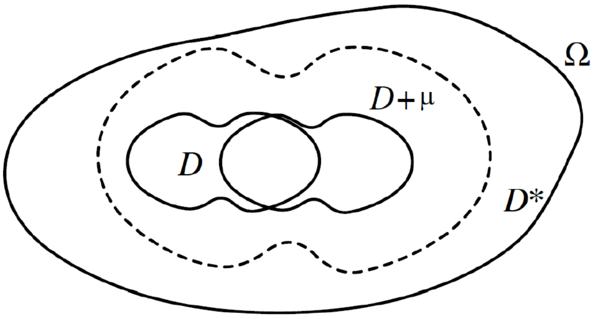 Figure 1
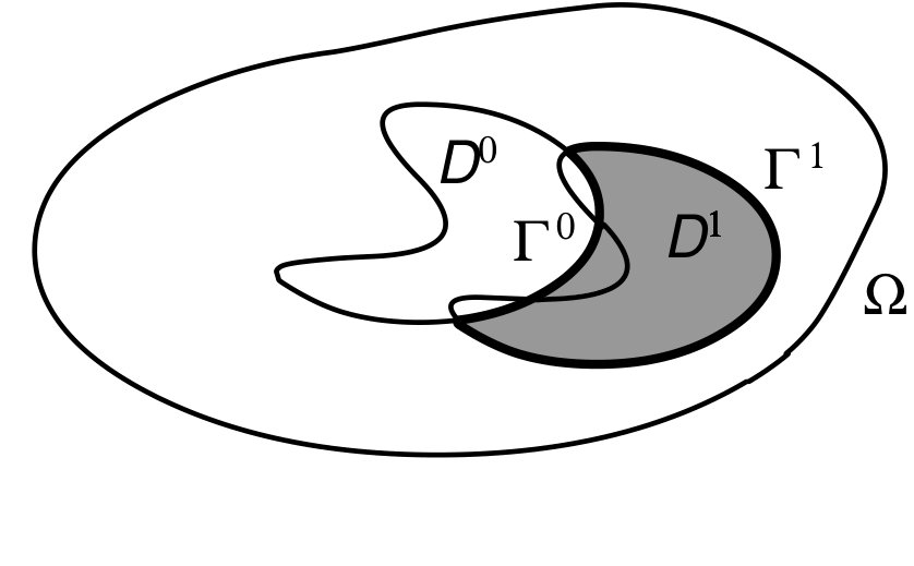 Figure 2
Peer Reviews
No public reviews on file for this paper yet. If you reviewed it on a platform where reviews are public (OpenReview, ICLR, NeurIPS, ICML), you can paste yours below so the community can read it here.
Videos
No videos yet. Explain this paper in a talk, walkthrough, or lecture? Add one.
On Some Geometric Inverse Problems for Nonscalar Elliptic Systems
Raul K.C. Araújo Department of Mathematics, Federal University of Pernambuco, UFPE, CEP 50740-545, Recife, PE, Brazil. E-mail: [email protected]. Partially supported by CNPq (Brazil).
Enrique Fernández-Cara University of Sevilla, Dpto. E.D.A.N, Aptdo 1160, 41080 Sevilla, Spain. E-mail: [email protected]. Partially supported by grant MTM--P, Ministry of Economy and Competitiveness (Spain).
Diego A. Souza Department of Mathematics, Federal University of Pernambuco, UFPE, CEP 50740-545, Recife, PE, Brazil. E-mail: [email protected]. Partially supported by CNPq (Brazil) by the grants /-1 and Propesq (UFPE)- Edital Qualis A.
Abstract
In this paper, we consider several geometric inverse problems for linear elliptic systems. We prove uniqueness and stability results. In particular, we show the way that the observation depends on the perturbations of the domain. In some particular situations, this provides a strategy that could be used to compute approximations to the solution of the inverse problem. In the proofs, we use techniques related to (local) Carleman estimates and differentiation with respect to the domain.
Keywords and phrases: inverse problems, nonscalar elliptic systems, unique continuation, domain variation techniques, reconstruction.
Mathematics Subject Classification: 35J55, 65N21, 65M32, 49K40.
1 Introduction
Let be a simply connected bounded domain whose boundary is of class , let be a fixed nonempty open set with and let be a nonempty open set. In what follows, the symbols will be used to denote generic positive constants. Sometimes, we will indicate the data on which they depend by writting (for example)
Let us consider the following family of subsets of :
[TABLE]
and let us denote by the set of all such that and
[TABLE]
for some with , where is the smallest positive constant such that
[TABLE]
In this paper, we will always assume that and . Under these circumstances it is well known that, for any there exists a unique solution to the system
[TABLE]
furthermore satisfying
[TABLE]
In many physical phenomena, in order to predict the result of a measurement, we need a model of the system under investigation (typically a PDE system) and an explanation or interpretation of the observed quantities. If we are able to compute the solution to the model and quantify relevant observations, we say that we have solved the forward or direct problem. Contrarily, the inverse problem consists of using the observations to recover unknown data that characterize the model. For details about the main questions concerning inverse problems for PDEs from the theoretical and numerical viewpoints, see for instance the book [11].
In this paper, we will deal with the following inverse geometric problem:
Given and , find a set such that the solution to the linear system (2) satisfies the additional conditions:
[TABLE]
A motivation of problems of this kind can be found, for instance, when one tries to compute the stationary temperature of a chemically reacting plate whose shape is unknown. More precisely, (2)-(3) has the following interpretation: assume that a chemical product, sensible to temperature effects, fills an unknown domain ; its concentration and its temperature are imposed on the whole outer boundary the associated normal fluxes are measured on and both and vanish on the boundary of the non-reacting unknown set ; what we pretend to do is to determine from these data and measurements.
In the context of the inverse problem (2)-(3), three main questions appear. They are the following:
- •
Uniqueness: Let and be two observations and let and be solutions to (2) satisfying the identities (3) associated to the sets and , respectively. The question is: do we have whenever ?
- •
Stability: Find an estimate of the “distance” from to in terms of the “distance” from to of the form
[TABLE]
where the function satisfies as , valid at least whenever and are “close” to a fixed .
- •
Reconstruction: Find an iterative algorithm to compute the unknown domain from the observation .
In this paper, we focus on the uniqueness and the stability of the inverse problem (2)-(3). Specifically, our first main result is the following:
Theorem 1**.**
Assume that is nonzero. For , let be the unique weak solution to (2) with replaced by and let and be given by the corresponding equalities (3). Then one has the following:
[TABLE]
The proof is given in Section 2. It relies on some ideas from [9]; more precisely, we use two well known properties of (2): unique continuation and well-posedness in the Sobolev space .
Remark 1**.**
Note that, if then the associated solution to (2) is zero, for any . Therefore, the uniqueness problem has no sense when . **
Remark 2**.**
In the one-dimensional case, if one consider (2) with only one boundary observation, uniqueness may not hold. Indeed, suppose that , and consider the system
[TABLE]
where (all them different from zero) and . Then, and, using the parameter variation method, we get that a solution to (4) is given by
[TABLE]
for each . Therefore, if we have and this implies non-uniqueness.
For , the uniqueness in the N-dimensional case with only one information on is, to our knowledge, an open question. * *
In order to state our main stability result, let us introduce some notation. Thus, let be a fixed subdomain, let satisfy
[TABLE]
and, for any , let us denote by , and respectively the mapping , the open set and the solution to (2) with replaced by . For simplicity, it will be assumed that the coefficients are constant. The following holds:
Theorem 2**.**
There exists with the following properties:
The mapping
[TABLE]
is well defined and analytic in , with values in . 2. 2.
Either for all (and then the mapping in (5) is constant), or there exist , and (an integer) such that
[TABLE]
In [12] and [4], a similar geometric inverse problem for one scalar elliptic equation is studied. For geometric inverse problems for nonlinear models, like Stokes, Navier-Stokes and Boussinesq systems, the uniqueness has been analyzed in [1], [8] and [7], respectively. Reconstruction algorithms have been considered and applied in [2] and [3] for the stationary Stokes system and in [8] and [7] for the Navier-Stokes and Boussinesq systems.
Note that, in the applications to fluid mechanics, the goal is to identify the shape of a body around which a fluid flows from measurements performed far from the body. In other contexts, the domain can represent a rigid body immersed in an elastic medium. Thus, related inverse problems with relevant applications in Elastography have been analyzed in [5] for the wave equation and [6] for the Lamé system.
This paper is organized as follows. In Section 2, we prove a unique continuation property for the solutions to (2) and, then, we prove the uniqueness result (Theorem 1). Section 3 is devoted to proof of the stability result (Theorem 2). Finally, in Section 4, we present some additional comments and open questions.
2 Unique continuation and uniqueness
In this section, we analyze a unique continuation property for (2). More precisely, we have the following result:
Theorem 3**.**
Let be a bounded domain whose boundary is of class , let be a nonempty open set and assume that . Then, any solution to the linear system
[TABLE]
satisfying
[TABLE]
*is zero everywhere. *
As already mentioned, the proof relies on some ideas from [9]. In fact, we will divide the proof in two parts: (i) the proof of Theorem 3 when and are open balls and (ii) the proof for general domains and , using a compactness argument.
2.1 A unique continuation property for balls
In this Section, we prove a very particular result concerning the unique continuation of the solutions to (6):
Lemma 1**.**
Assume that , and , where denotes the open ball of radius centered at . For any solution to the linear system (6) in , the following property holds:
[TABLE]
Before proving this lemma, let us introduce and let us define
[TABLE]
Let us also recall that the Poisson bracket of and is given by
[TABLE]
A crucial result in the proof of Lemma 1 is the following:
Theorem 4** ([9, Proposition ]).**
Let be a nonempty bounded open set, a nonempty compact set and assume that . Suppose that is bi-convex in with respect to the characteristics of and , i.e. satisfies the following:
[TABLE]
Then, there exist and such that, for all and any function , one has:
[TABLE]
Proof of Lemma 1.
Without loss of generality we may assume that . Let be a solution to (6) such that and in .
We will try to apply Theorem 4 to the functions and . To do this, let us fix and let us introduce the sets
[TABLE]
and a function with
[TABLE]
It is not difficult to see that
[TABLE]
where the are the Kronecker symbols. From (9) and (10), we have that
[TABLE]
for any such that . Therefore, we see that (8) is satisfied by the function in
Let us introduce a cut-off function satisfying for and let us set and . It is then clear that . After some computations, we obtain that:
[TABLE]
where
[TABLE]
Consequently, we can apply Theorem 4 to and deduce that there exist and such that
[TABLE]
for all . Here, we have absorbed the lower order term for from the right hand side by taking small enough. Analogously, there exist positive constants and such that,
[TABLE]
for all .
Next, adding (12) and (13), taking sufficiently small and sufficiently large and absorbing again the lower order terms for and from the right hand side, we have
[TABLE]
for all .
To conclude the proof, we note that (11), the fact that in and for imply that and vanish in . Now, we have from (9) that is positive and radially decreasing in . Thus, one has
[TABLE]
On the other hand,
[TABLE]
It follows from (14)–(16) that
[TABLE]
Since and are independent of and , we can let and get that
[TABLE]
and, consequently, and vanish in . Since is arbitrarily small, we conclude that and vanish identically in .
2.2 Unique continuation for general domains
The goal of this section is to prove Theorem 3 in the general case.
Let be a solution to (6) satisfying (7) and let us assume that . Let be a point of and let us see that and in a neighborhood of .
Since is connected, there exists a curve such that and .
Notice that for any there exists such that . Since is a compact set, there exist and satisfying
[TABLE]
By construction, setting , we have that , for all .
Finally, we set and fix . It is clear that vanishes in whence, by Lemma 1, also vanishes in . Let . Then, we have that in and, in view of Lemma 1, in . Applying the same idea a finite number of times, we obtain and in This ends the proof.
2.3 Proof of Theorem 1: uniqueness
Let us introduce the open sets and and let be the unique connected component of such that . Also, let us set and in . Since and , the couple satisfies:
[TABLE]
Now, we fix and we choose such that . Let us set and consider the extension by zero of to the whole set .
From (17), it follows that
[TABLE]
Also, since is connected and in , Theorem 3 implies in . In particular, in .
To conclude, let us prove that and must be empty. Thus, let us suppose that and let us introduce the set . By hypothesis, is nonempty. On the other hand, note that , where and (see Figure 1).
Therefore, since in , the pair verifies
[TABLE]
Since the linear system (18) possesses exactly one solution, we necessarily have in . Consequently, in view of Theorem 3, in This contradicts the fact that is not identically zero on . Hence, is the empty set.
Analogously, one can prove that is empty and, finally, one has .
3 Stability
3.1 Preliminary results
Let us introduce some basic notation. Let be given and let us set
[TABLE]
In the sequel, we will consider the set
[TABLE]
where . We will work with mappings of the form , where is the identity and . For any , is obviously bijective, (see [10], p. 193) and
[TABLE]
Also, the corresponding functions , and satisfy
[TABLE]
Let and be given, let us set again and and let us consider the solution to
[TABLE]
Since , there exists such that
[TABLE]
Thus, we can write , where is the solution to
[TABLE]
and
[TABLE]
We see from (20) that for any the following holds:
[TABLE]
Let us introduce the functions:
[TABLE]
where is the isomorphism from onto induced by , that is,
[TABLE]
Observe that, since in and in , we have in . In other words, is invariant under the isomorphism associated to .
It can be easily shown that solving the variational problem (21) is equivalent to find such that
[TABLE]
for all that is, a solution to the system:
[TABLE]
where is given by
[TABLE]
For convenience, we will rewrite (22) in the abridged form
[TABLE]
where the notation is self-explanatory.
Lemma 2**.**
The linear operator is an isomorphism. Furthermore, if denotes the usual norm in , one has
[TABLE]
Proof.
It is easy to see that and . On the other hand, the bilinear form , given by
[TABLE]
is coercive in view of (19). Indeed, one has
[TABLE]
for all .
Therefore, from Lax-Milgram’s Lemma, we get the result.
Theorem 5**.**
*The mapping is analytic in a neighbourhood of the origin in . *
Proof.
We note first that does not depend of , because where . Then, since the mapping is a isomorphism we have by (23) that
[TABLE]
From the results in [10, 15], we know that the mapping is analytic in a neighbourhood of [math]. Consequently, this is also the case for and the proof is done.
3.2 Proof of Theorem 2: stability
Let and be given, with in . Recall that, in Theorem 2, for any , we have set and and is the solution to
[TABLE]
We will argue as in [1]:
First, it follows from Theorem 5 and the fact that in that there exists such that the mapping in (5) is well defined and analytic in . Hence, there exist in such that
[TABLE]
where the series converges in . 2. 2.
Now, let us assume that for some . In view of Theorem 1, not all the can be zero. Let be the smallest such that . It is then clear that there exists such that
[TABLE]
Accordingly, for these , one must also have
[TABLE]
which allows to achieve the proof.
4 Additional comments and questions
4.1 A similar inverse problem with internal observation
Let be a nonempty open set. Consider the following geometric inverse problem, where the observation is performed on :
Given and , find a set such that the solution to the linear system (2) satisfies the following additional condition:
[TABLE]
We have the following uniqueness result:
Theorem 6**.**
Assume that is nonzero and suppose that there exists a nonempty open set such that a.e. in . Let be the unique weak solution to (2) with replaced by for and let be given by the corresponding equality (26). Then, one has:
[TABLE]
Proof.
The proof is very similar to the proof of Theorem 1.
As before, we can consider the open sets , and the unique connected component of such that . Again, let us set and in . Then, using the facts that and a.e. in , we have that and satisfies
[TABLE]
and
[TABLE]
Consequently, Theorem 3 guarantees that in . Arguing as in the proof of Theorem 1, we deduce that and are empty sets and, consequently, .
We also have a stability result similar to Theorem 2. Thus, let us fix and with in , let us take and and let be the solution to (24). The following holds:
Theorem 7**.**
Under the assumptions in Theorem 6 on and , there exists with the following properties:
The mapping
[TABLE]
is well defined and analytic in , with values in . 2. 2.
Either for all (and then the mapping in (27) is constant), or there exist , and (an integer) such that
[TABLE]
Proof.
Again, the proof is very similar to the proof of stability in the boundary observation case (Theorem 2). In fact, the unique difference appears in the last part of the argument, when we write
[TABLE]
instead of (25).
For brevity, we omit the details.
Remark 3**.**
Recall that, in the case of problem –, we need two boundary observations, the normal derivatives of and on , to deduce uniqueness and stability. The last two results show that, with internal observations, this holds with the information supplied by just one variable. * *
4.2 A geometric inverse problem for a parabolic system
Let us present some ideas that allow to extend Theorems 1 and 6 to time-dependent parabolic systems. For brevity, we will only consider the boundary observation case. Thus, let be given and let us consider the following inverse problem:
Given and in appropriate spaces and a nonempty open set , find an open set such that the solution to the linear evolution system:
[TABLE]
satisfies the additional conditions:
[TABLE]
If one assume that , then arguments similar to those in the proof of Theorem 1 can be used to deduce uniqueness for (28)–(29).
Indeed, the first step is to deduce a unique continuation property:
Proposition 1**.**
Let be a bounded domain whose boundary is of class and let us set . Suppose that and let be a nonempty open subset of . Then, any solution to
[TABLE]
satisfies the following property:
[TABLE]
where is the horizontal component of , defined by
[TABLE]
The proof of this result is similar to the proof of Theorem 1.4 in [9].
Remark 4**.**
Let be an open nonempty subset of . Then, any solution to (30) satisfies the following property:
[TABLE]
Indeed, take . Since is open in , there exist constants such that . Let us denote by the extension by zero of to . Then, is a solution to (30) in and in . Consequently, by Proposition 1, vanishes in . Since is arbitrary in , we get the result. * *
Let us now achieve the proof of uniqueness for the geometric inverse problem (28)-(29). To this end, let and be two open sets in and let be the solution to (28) with . Let us also assume that
[TABLE]
As before, by introducing the open sets , and , with and , we have
[TABLE]
From Remark 4, we find that in .
We can prove that is the empty set. Indeed, suppose the contrary, i.e. that is nonempty. Let us introduce the open set . As before, using the fact that in , we see that
[TABLE]
Consequently, thanks to the uniqueness of solution to (31) and Proposition 1, we must have in , which implies , an absurd. This proves that .
Similarly, we can also prove that and, therefore, .
Remark 5**.**
If, in (28), we impose nonzero initial conditions on and/or , the situation is much more complex. In particular, the prevuious argument does not work. A detailed analysis will be the objective of a forthcoming paper. * *
Remark 6**.**
Notice that, in this time-dependent case, no assumption of the kind (1) is needed. * *
Stability results like Theorems 2 and 7 can also be established in this framework. We will not give the details for brevity, since the arguments are not very different and can easily be completed by the reader.
4.3 Additional comments on stability
In the context of the stability problem, we can adopt another (more geometrical) viewpoint. To clarify the situation, let us consider the scalar systems
[TABLE]
where , is as before, and are convex and have nonempty intersection and the following regularity properties hold:
[TABLE]
Let us assume that
[TABLE]
Then, it can be proved that the Haussdorf distance satisfies the estimate
[TABLE]
where only depends on , and ; see [4].
The proof is based on the following well-posedness results, where is as above:
- •
Let us set again and let us assume that
[TABLE]
Then, under the previous hypotheses, one has .
- •
Assume that . Then .
Under additional properties for the , and , the previous estimates can be improved; see [4] for more details.
It would be interesting to extend this approach to the inverse problems (2), (3) and (2), (26). At present, to our knowledge, whether or not this is possible is an open question.
4.4 Reconstruction
As already said, reconstruction algorithms for the solution of problems of the kind (2)–(3) have been considered in several papers. In all them, the main idea is to reduce to finite dimension and reformulate the search of the unknown as a constrained (maybe numerically ill-conditionned) extremal problem. Then, usual gradient, quasi-Newton or even Newton methods can be used to compute approximate solutions; see for instance [1, 2, 3].
Let us present in this section a different approach that relies on the domain variation techniques introduced in [13, 14, 15].
The main idea is to describe how the observation depends on small perturbations of as explicitly as possible. Thus, for each , let us set
[TABLE]
and let us recall that, whenever , we also have as indicated in Figure 2 below.
Let us assume that satisfy (1) and we can consider the perturbed system
[TABLE]
Assuming appropriate regularity hypothesis on and , it can be proved that
[TABLE]
where is the unique solution to the linear system
[TABLE]
and
[TABLE]
Moreover, for any , one has
[TABLE]
where is the solution to the adjoint system
[TABLE]
Let us see how, starting from an already computed candidate to the solution of the geometric inverse problem (2)–(3), we can compute a better candidate of the form .
Let be a finite dimensional subspace of and let be a basis of . We will take such that . Then, we can write
[TABLE]
for some to be determined.
Now, let us introduce linearly independent functions . Using (32), we obtain
[TABLE]
where
[TABLE]
we have denoted by is the solution to (33) corresponding to and is the observation corresponding to . We thus see that an appropriate strategy to compute the coefficients is to solve, if possible, the finite-dimensional algebraic system
[TABLE]
A rigorous justification of the main steps presented before, together with a detailed analysis of the reconstruction method, will be the subject of a forthcoming work.
Acknowledgments: This work has been partially done while the first author was visiting the University of Sevilla (Spain). He wishes to thank the members of the IMUS (Institute of Mathematics of the University of Sevilla) for their kind hospitality.
The reference list from the paper itself. Each links out to its DOI / PubMed record.
- 1[1] C. Alvarez, C. Conca, L. Friz, O. Kavian, Identification of immersed obstacles via boundary measurements, Inverse Problems , 21 (2005), 1531-1552.
- 2[2] C.Alvarez, C. Conca, R. Lecaros and J.H. Ortega, On the identification of a rigid body immersed in a fluid: A numerical approach, Engineering Analysis with Boundary Elements , 32 (2008), 919-925.
- 3[3] A. Ben Abda, M. Hassine,M. Jaoua and M. Masmoudi, Topological sensitivity analysis for the location of small cavities in Stokes flow, SIAM J. Control Optim , 48 (2009), 2871-2900.
- 4[4] A.L: Buckgeim, J: Cheng, M: Yamamoto, Stability for an inverse boundary problem of determining a part of a boundary. Inverse Problems, 1999, 15(4):1021-1032.
- 5[5] A. Doubova and E. Fernández-Cara, Some geometric inverse problems for the linear wave equations, Inverse Problems and Imaging , 9 (2015), 371-393.
- 6[6] A. Doubova and E. Fernández-Cara, Some geometric inverse problems for the Lamé system with applications in elastography, Appl. Math. Optim. , 76 (2018), 1-21.
- 7[7] A. Doubova, E. Fernández-Cara, M. González-Burgos and J.H. Ortega, A geometric inverse problem for the Boussinesq system, Discret. Contin. Dyn. Syst. Ser. B , 6 (2006), 1213-1238.
- 8[8] A. Doubova, E. Fernández-Cara and J.H. Ortega, On the identification of a single body immersed in a Navier-Stokes fluid, Eur. J. Appl. Math. , 18 (2007), 57-80.