The Commute Trip Sharing Problem
Mohd Hafiz Hasan, Pascal Van Hentenryck, Antoine Legrain

TL;DR
This paper formalizes the Commute Trip Sharing Problem (CTSP) to optimize carpooling by matching riders and drivers, introducing exact algorithms, and demonstrating significant potential reductions in vehicle usage and miles traveled.
Contribution
It introduces the CTSP, a comprehensive vehicle routing model for ride sharing, and develops two exact algorithms to solve it efficiently.
Findings
Algorithms solve small and medium problems optimally.
Carpooling can reduce vehicle usage by up to 57%.
Vehicle miles traveled can decrease by up to 46%.
Abstract
Parking pressure has been steadily increasing in cities as well as in university and corporate campuses. To relieve this pressure, this paper studies a car-pooling platform that would match riders and drivers, while guaranteeing a ride back and exploiting spatial and temporal locality. In particular, the paper formalizes the Commute Trip Sharing Problem (CTSP) to find a routing plan that maximizes ride sharing for a set of commute trips. The CTSP is a generalization of the vehicle routing problem with routes that satisfy time window, capacity, pairing, precedence, ride duration, and driver constraints. The paper introduces two exact algorithms for the CTPS: A route-enumeration algorithm and a branch-and-price algorithm. Experimental results show that, on a high-fidelity, real-world dataset of commute trips from a mid-size city, both algorithms optimally solve small and medium-sized…
Click any figure to enlarge with its caption.
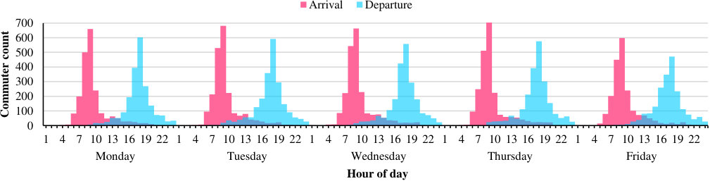 Figure 1
 Figure 2
 Figure 3
 Figure 4
 Figure 5
 Figure 6
 Figure 7
 Figure 8
 Figure 9
 Figure 10
 Figure 11
 Figure 12
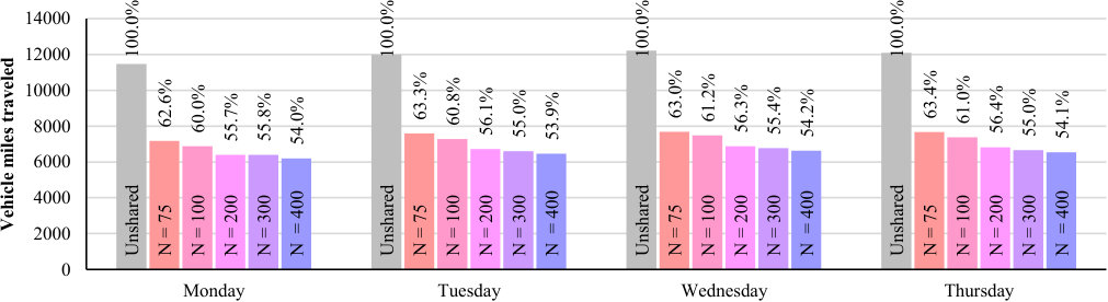 Figure 13
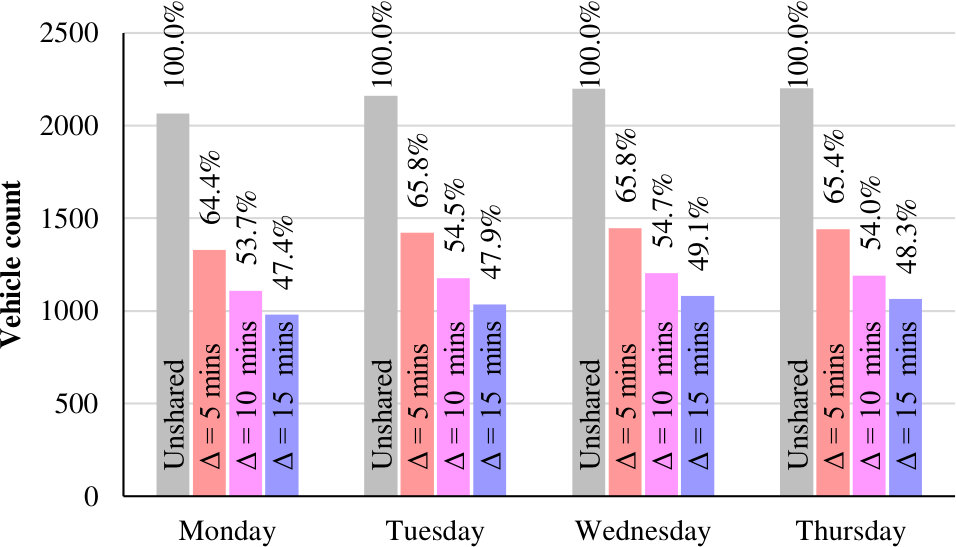 Figure 14
 Figure 15
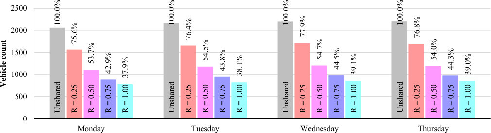 Figure 16
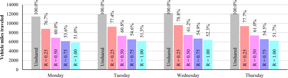 Figure 17
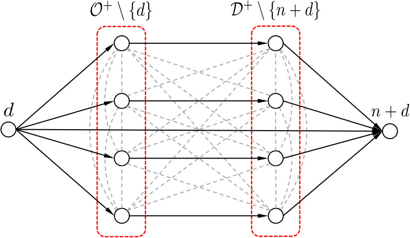 Figure 18
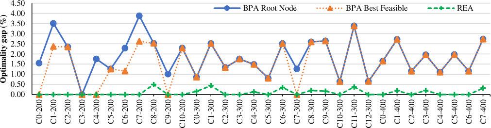 Figure 19
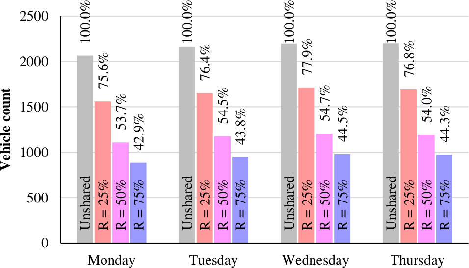 Figure 20
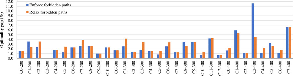 Figure 21
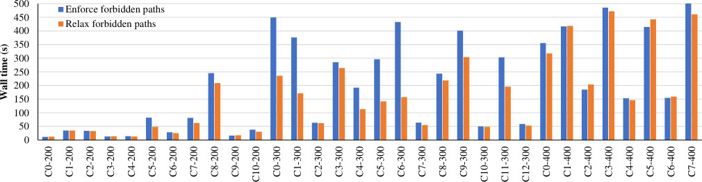 Figure 22
 Figure 23
 Figure 24
 Figure 25
 Figure 26
 Figure 27
 Figure 28
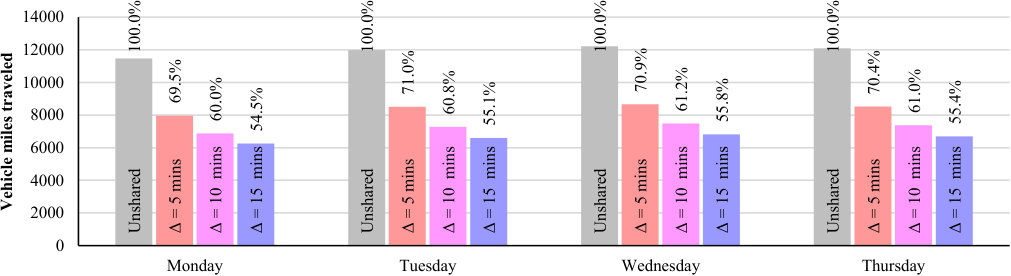 Figure 29
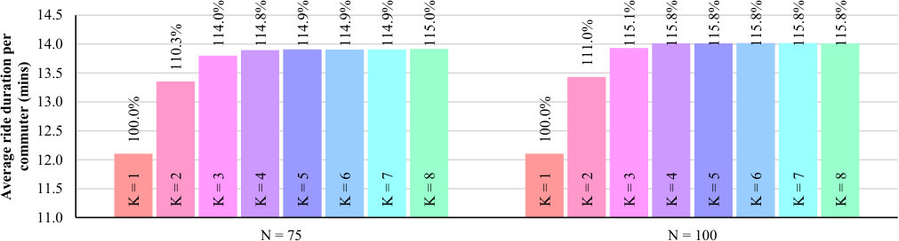 Figure 30
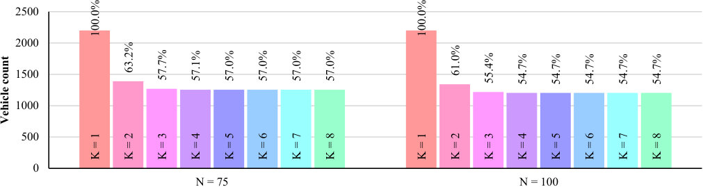 Figure 31
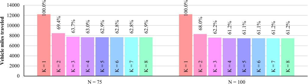 Figure 32
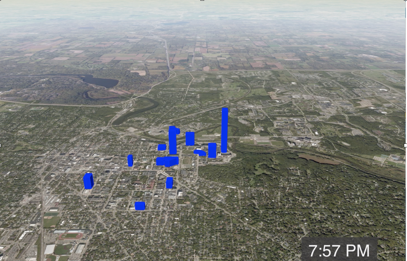 Figure 33
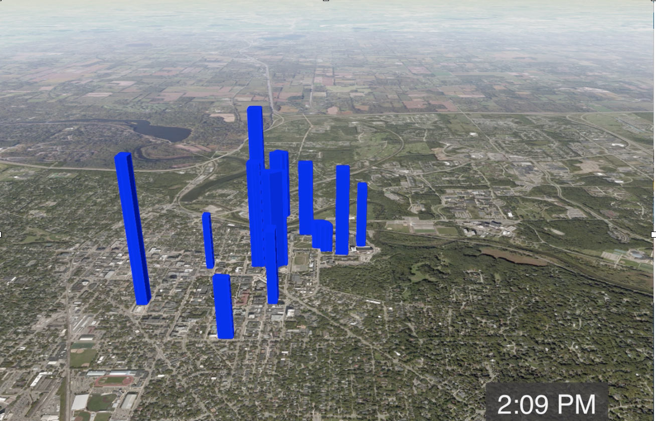 Figure 34
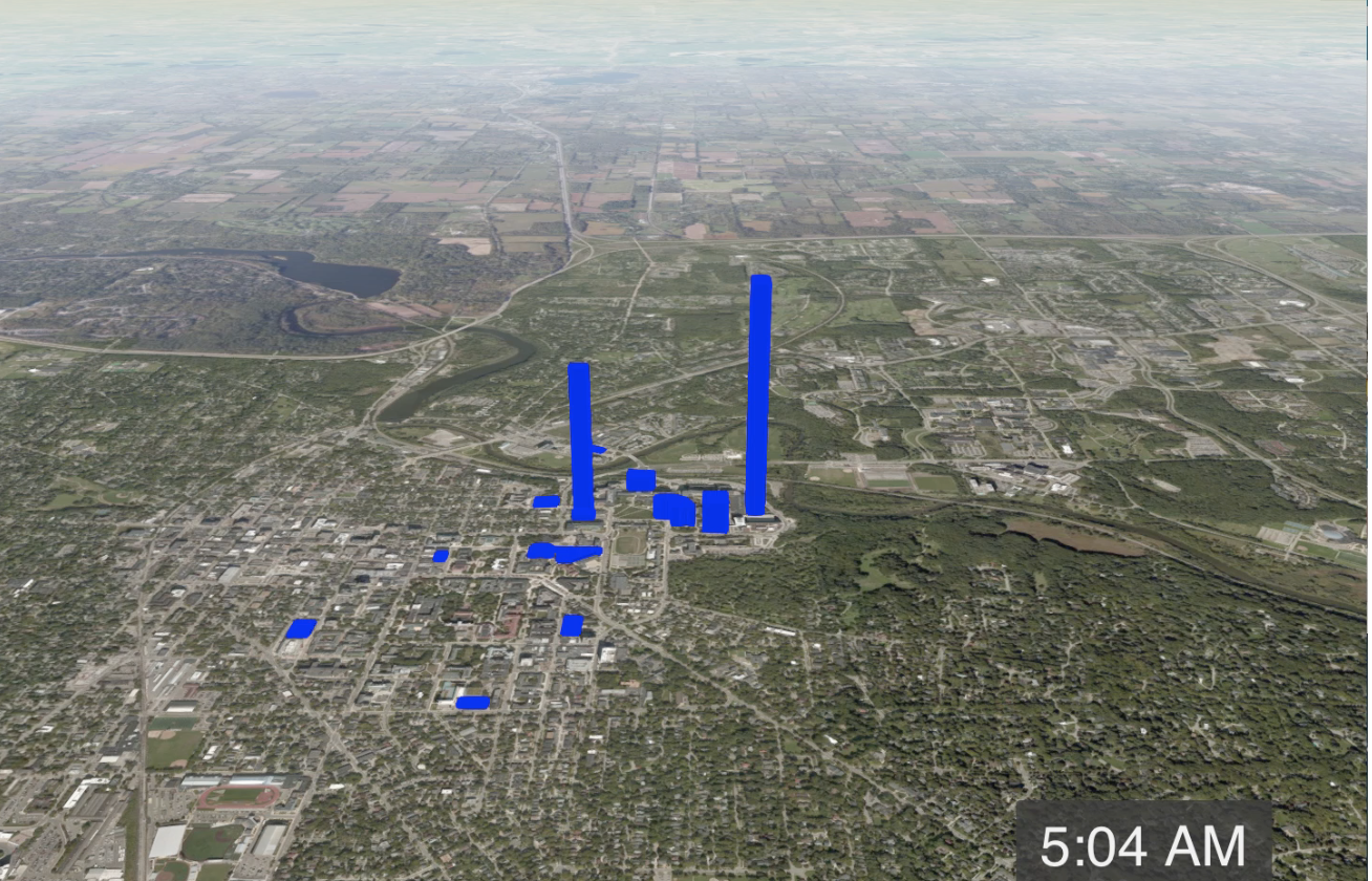 Figure 35
| \up\down Cluster size | Vehicle capacity | Cluster ID | Column # | Vehicle # | Total distance (m) | Optimality gap (%) | Wall time (s) | |
|---|---|---|---|---|---|---|---|---|
|
Total | |||||||
| \up100 | 4 | C0-100 | 854 | 63 | 488119 | 0.00 | 34 | 34 |
| C1-100 | 456 | 75 | 331497 | 0.00 | 31 | 31 | ||
| C2-100 | 3802 | 46 | 596824 | 0.00 | 36 | 36 | ||
| C3-100 | 4510 | 46 | 586434 | 0.00 | 35 | 36 | ||
| C4-100 | 4232 | 44 | 558323 | 0.00 | 35 | 41 | ||
| C5-100 | 732 | 70 | 366565 | 0.00 | 31 | 31 | ||
| C6-100 | 2579 | 47 | 724844 | 0.00 | 35 | 35 | ||
| C7-100 | 2020 | 53 | 661648 | 0.00 | 34 | 34 | ||
| C8-100 | 1803 | 51 | 609120 | 0.00 | 34 | 34 | ||
| C9-100 | 12034 | 40 | 527217 | 0.00 | 36 | 38 | ||
| C10-100 | 1095 | 58 | 426386 | 0.00 | 34 | 34 | ||
| C11-100 | 2374 | 51 | 427829 | 0.00 | 34 | 35 | ||
| C12-100 | 989 | 62 | 413012 | 0.00 | 33 | 33 | ||
| C13-100 | 909 | 61 | 483087 | 0.00 | 34 | 34 | ||
| C14-100 | 4306 | 40 | 693825 | 0.00 | 35 | 40 | ||
| C15-100 | 4605 | 48 | 790005 | 0.00 | 34 | 37 | ||
| C16-100 | 1578 | 55 | 627423 | 0.00 | 33 | 33 | ||
| C17-100 | 1151 | 60 | 640945 | 0.00 | 33 | 33 | ||
| C18-100 | 952 | 58 | 681240 | 0.00 | 34 | 34 | ||
| C19-100 | 2226 | 51 | 503252 | 0.00 | 34 | 35 | ||
| C20-100 | 4254 | 46 | 569724 | 0.00 | 35 | 36 | ||
| C21-100 | 667 | 78 | 328216 | 0.00 | 32 | 32 | ||
| 5 | C0-100 | 854 | 63 | 488119 | 0.00 | 1185 | 1186 | |
| C1-100 | 456 | 75 | 331497 | 0.00 | 1072 | 1072 | ||
| C2-100 | 3910 | 46 | 596658 | 0.00 | 1356 | 1357 | ||
| C3-100 | 4814 | 46 | 584077 | 0.00 | 1357 | 1359 | ||
| C4-100 | 4487 | 44 | 552862 | 0.00 | 1298 | 1342 | ||
| C5-100 | 735 | 70 | 366565 | 0.00 | 1034 | 1034 | ||
| C6-100 | 2596 | 47 | 724844 | 0.00 | 1362 | 1362 | ||
| C7-100 | 2043 | 53 | 661528 | 0.00 | 1326 | 1326 | ||
| C8-100 | 1842 | 51 | 609038 | 0.00 | 1317 | 1317 | ||
| C9-100 | 16749 | 40 | 519564 | 0.00 | 1419 | 1451 | ||
| C10-100 | 1096 | 58 | 426386 | 0.00 | 1254 | 1254 | ||
| C11-100 | 2418 | 51 | 427829 | 0.00 | 1320 | 1321 | ||
| C12-100 | 990 | 62 | 413012 | 0.00 | 1208 | 1208 | ||
| C13-100 | 912 | 61 | 483087 | 0.00 | 1221 | 1221 | ||
| C14-100 | 4448 | 40 | 689319 | 0.00 | 1383 | 1457 | ||
| C15-100 | 5985 | 48 | 788340 | 0.00 | 1287 | 1294 | ||
| C16-100 | 1599 | 55 | 626787 | 0.00 | 1226 | 1227 | ||
| C17-100 | 1155 | 60 | 640945 | 0.00 | 1218 | 1218 | ||
| C18-100 | 953 | 58 | 681240 | 0.00 | 1292 | 1293 | ||
| C19-100 | 2291 | 51 | 503252 | 0.00 | 1352 | 1352 | ||
| C20-100 | 4761 | 46 | 568797 | 0.00 | 1352 | 1354 | ||
| C21-100 | 667 | 78 | 328216 | 0.00 | 1080 | 1080 | ||
| 6 | C0-100 | 854 | 63 | 488119 | 0.00 | 25088 | 25088 | |
| C1-100 | 456 | 75 | 331497 | 0.00 | 20117 | 20117 | ||
| C2-100 | 3917 | 46 | 596658 | 0.00 | 33455 | 33456 | ||
| C3-100 | 4872 | 46 | 584048 | 0.00 | 33801 | 33802 | ||
| C4-100 | 4510 | 44 | 552862 | 0.00 | 29993 | 30180 | ||
| C5-100 | 735 | 70 | 366565 | 0.00 | 18613 | 18613 | ||
| C6-100 | 2598 | 47 | 724844 | 0.00 | 43135 | 43136 | ||
| C7-100 | 2043 | 53 | 661528 | 0.00 | 38791 | 38792 | ||
| C8-100 | 1848 | 51 | 609038 | 0.00 | 39437 | 39437 | ||
| C9-100 | 18758 | 40 | 517624 | 0.00 | 48359 | 48403 | ||
| C10-100 | 1096 | 58 | 426386 | 0.00 | 36941 | 36941 | ||
| C11-100 | 2419 | 51 | 427829 | 0.00 | 39761 | 39763 | ||
| C12-100 | 990 | 62 | 413012 | 0.00 | 31038 | 31038 | ||
| C13-100 | 912 | 61 | 483087 | 0.00 | 33881 | 33881 | ||
| C14-100 | 4456 | 40 | 689319 | 0.00 | 41455 | 41492 | ||
| C15-100 | 6939 | 48 | 788340 | 0.00 | 36980 | 36990 | ||
| C16-100 | 1600 | 55 | 626787 | 0.00 | 32031 | 32031 | ||
| C17-100 | 1155 | 60 | 640945 | 0.00 | 34810 | 34810 | ||
| C18-100 | 953 | 58 | 681240 | 0.00 | 38501 | 38501 | ||
| C19-100 | 2294 | 51 | 503252 | 0.00 | 42573 | 42574 | ||
| C20-100 | 4898 | 46 | 568797 | 0.00 | 43900 | 43903 | ||
| \down | C21-100 | 667 | 78 | 328216 | 0.00 | 29507 | 29507 | |
| \up\down Cluster size | Vehicle capacity | Cluster ID | Inbound edge # | Outbound edge # | Tree node # | Column # | Vehicle # | Total distance (m) | Optimality gap (%) | Integrality gap (%) | Wall time (s) | |||||||
|---|---|---|---|---|---|---|---|---|---|---|---|---|---|---|---|---|---|---|
|
|
|
|
|
Total | |||||||||||||
| \up75 | 7 | C0-75 | 1661 | 1565 | 15 | 463 | 47 | 356296 | 0.00 | 0.00 | 0.00 | 1 | 1 | 1 | 1 | |||
| C2-75 | 1906 | 1405 | 79 | 1072 | 40 | 643540 | 0.02 | 0.00 | 0.01 | 3 | 3 | 30 | 39 | |||||
| C3-75 | 3099 | 1809 | 21 | 1238 | 38 | 487061 | 0.00 | 0.00 | 0.00 | 4 | 4 | 4 | 20 | |||||
| C4-75 | 2052 | 1851 | 139 | 962 | 43 | 398216 | 2.27 | 0.00 | 0.01 | 1 | 2 | 33 | 33 | |||||
| C5-75 | 823 | 810 | 1 | 267 | 61 | 230460 | 0.00 | 0.00 | 0.00 | 1 | 1 | 1 | 1 | |||||
| C6-75 | 3427 | 2012 | 33 | 1515 | 35 | 450414 | 2.85 | 0.00 | 2.85 | 48 | 48 | 186 | 247 | |||||
| C7-75 | 2458 | 1649 | 31 | 616 | 46 | 437743 | 2.17 | 0.00 | 2.17 | 1 | 1 | 1 | 3 | |||||
| C8-75 | 3002 | 2183 | 23 | 1025 | 37 | 487245 | 2.69 | 0.00 | 2.69 | 2 | 2 | 9 | 18 | |||||
| C9-75 | 3550 | 2341 | 189 | 2347 | 31 | 327993 | 3.22 | 0.00 | 3.22 | 20 | 20 | 482 | 594 | |||||
| C10-75 | 2856 | 1580 | 2 | 1459 | 32 | 525115 | 3.12 | 3.12 | 3.12 | 39153 | 39154 | 39154 | 43200 | |||||
| C11-75 | 1955 | 1193 | 24 | 650 | 47 | 443770 | 0.00 | 0.00 | 0.00 | 1 | 1 | 1 | 3 | |||||
| C12-75 | 1801 | 1347 | 5 | 502 | 46 | 298162 | 0.00 | 0.00 | 0.00 | 1 | 1 | 1 | 1 | |||||
| C13-75 | 2699 | 1302 | 337 | 1470 | 37 | 479166 | 2.70 | 0.00 | 2.70 | 2 | 3 | 78 | 105 | |||||
| C14-75 | 2045 | 1332 | 19 | 619 | 47 | 301108 | 0.00 | 0.00 | 0.00 | 1 | 1 | 2 | 2 | |||||
| C15-75 | 3007 | 1443 | 25 | 1089 | 36 | 460087 | 0.01 | 0.00 | 0.01 | 2 | 3 | 3 | 17 | |||||
| C17-75 | 1492 | 835 | 7 | 411 | 50 | 348581 | 0.00 | 0.00 | 0.00 | 1 | 1 | 1 | 1 | |||||
| C19-75 | 1497 | 664 | 1 | 390 | 57 | 245827 | 0.00 | 0.00 | 0.00 | 1 | 1 | 1 | 1 | |||||
| C20-75 | 2323 | 1254 | 11 | 672 | 46 | 420825 | 0.00 | 0.00 | 0.00 | 1 | 1 | 2 | 2 | |||||
| C22-75 | 3113 | 1524 | 161 | 1382 | 40 | 472040 | 2.50 | 0.00 | 2.49 | 3 | 3 | 52 | 79 | |||||
| C23-75 | 2069 | 1548 | 23 | 940 | 35 | 379234 | 2.84 | 0.00 | 2.84 | 3 | 3 | 12 | 19 | |||||
| C24-75 | 2446 | 1694 | 745 | 1666 | 37 | 425806 | 5.25 | 0.00 | 2.70 | 3 | 6 | 148 | 329 | |||||
| C26-75 | 1957 | 1039 | 17 | 430 | 52 | 333692 | 0.00 | 0.00 | 0.00 | 1 | 1 | 1 | 1 | |||||
| C28-75 | 1781 | 1452 | 5 | 621 | 44 | 293838 | 0.00 | 0.00 | 0.00 | 1 | 1 | 1 | 1 | |||||
| C29-75 | 2495 | 2238 | 523 | 2052 | 32 | 543850 | 0.02 | 0.00 | 0.02 | 7 | 8 | 8 | 619 | |||||
| 8 | C0-75 | 1661 | 1565 | 15 | 461 | 47 | 356296 | 0.00 | 0.00 | 0.00 | 1 | 1 | 1 | 1 | ||||
| C2-75 | 1906 | 1405 | 75 | 1047 | 40 | 643540 | 0.02 | 0.00 | 0.01 | 2 | 2 | 26 | 36 | |||||
| C3-75 | 3099 | 1809 | 35 | 1268 | 38 | 487061 | 0.00 | 0.00 | 0.00 | 4 | 4 | 30 | 33 | |||||
| C4-75 | 2052 | 1851 | 101 | 928 | 43 | 398216 | 0.01 | 0.00 | 0.01 | 2 | 2 | 27 | 28 | |||||
| C5-75 | 823 | 810 | 1 | 267 | 61 | 230460 | 0.00 | 0.00 | 0.00 | 1 | 1 | 1 | 1 | |||||
| C6-75 | 3427 | 2012 | 62 | 1584 | 35 | 450414 | 5.54 | 0.00 | 2.85 | 39 | 40 | 266 | 362 | |||||
| C7-75 | 2458 | 1649 | 31 | 618 | 46 | 437743 | 2.17 | 0.00 | 2.17 | 1 | 1 | 1 | 2 | |||||
| C8-75 | 3002 | 2183 | 49 | 1064 | 37 | 487245 | 2.69 | 0.00 | 2.69 | 3 | 4 | 9 | 81 | |||||
| C9-75 | 3550 | 2341 | 105 | 2199 | 31 | 327993 | 3.22 | 0.00 | 3.22 | 26 | 27 | 300 | 398 | |||||
| C10-75 | 2856 | 1580 | 1 | 1425 | 32 | 525207 | 3.12 | 3.12 | 3.12 | 84928 | 84928 | 84928 | 84928 | |||||
| C11-75 | 1955 | 1193 | 24 | 641 | 47 | 443770 | 0.00 | 0.00 | 0.00 | 1 | 1 | 1 | 3 | |||||
| C12-75 | 1801 | 1347 | 5 | 508 | 46 | 298162 | 0.00 | 0.00 | 0.00 | 1 | 1 | 1 | 1 | |||||
| C13-75 | 2699 | 1302 | 427 | 1513 | 37 | 479166 | 2.70 | 0.00 | 2.70 | 4 | 4 | 77 | 144 | |||||
| C14-75 | 2045 | 1332 | 17 | 624 | 47 | 301108 | 0.00 | 0.00 | 0.00 | 1 | 1 | 1 | 2 | |||||
| C15-75 | 3005 | 1443 | 21 | 1093 | 36 | 460087 | 0.01 | 0.00 | 0.01 | 3 | 3 | 3 | 16 | |||||
| C17-75 | 1492 | 835 | 7 | 410 | 50 | 348581 | 0.00 | 0.00 | 0.00 | 1 | 1 | 1 | 1 | |||||
| C19-75 | 1497 | 664 | 1 | 390 | 57 | 245827 | 0.00 | 0.00 | 0.00 | 1 | 1 | 1 | 1 | |||||
| C20-75 | 2323 | 1254 | 11 | 671 | 46 | 420825 | 0.00 | 0.00 | 0.00 | 1 | 1 | 2 | 2 | |||||
| C22-75 | 3113 | 1524 | 161 | 1357 | 40 | 472040 | 2.50 | 0.00 | 2.49 | 3 | 4 | 65 | 103 | |||||
| C23-75 | 2069 | 1548 | 25 | 959 | 35 | 379234 | 2.84 | 0.00 | 2.84 | 4 | 4 | 16 | 22 | |||||
| C24-75 | 2446 | 1694 | 677 | 1567 | 37 | 425806 | 2.70 | 0.00 | 2.70 | 3 | 3 | 83 | 265 | |||||
| C26-75 | 1957 | 1039 | 15 | 430 | 52 | 333692 | 0.00 | 0.00 | 0.00 | 1 | 1 | 1 | 1 | |||||
| C28-75 | 1781 | 1452 | 5 | 620 | 44 | 293838 | 0.00 | 0.00 | 0.00 | 1 | 1 | 1 | 1 | |||||
| \down | C29-75 | 2495 | 2238 | 573 | 2163 | 32 | 543850 | 0.02 | 0.00 | 0.02 | 9 | 9 | 353 | 625 | ||||
| \up100 | 4 | C0-100 | 3488 | 1930 | 45 | 777 | 63 | 488119 | 0.00 | 0.00 | 0.00 | 2 | 2 | 2 | 5 | |||
| C1-100 | 1825 | 1642 | 5 | 429 | 75 | 331497 | 0.00 | 0.00 | 0.00 | 2 | 2 | 2 | 3 | |||||
| C2-100 | 5540 | 3106 | 1445 | 2652 | 46 | 596824 | 2.17 | 0.00 | 2.17 | 6 | 7 | 995 | 1397 | |||||
| C3-100 | 5383 | 3127 | 823 | 2794 | 46 | 586434 | 2.17 | 0.00 | 2.16 | 8 | 9 | 558 | 695 | |||||
| C4-100 | 4211 | 2787 | 50653 | 6120 | 44 | 558323 | 2.27 | 0.00 | 2.26 | 8 | 9 | 730 | 31745 | |||||
| C5-100 | 1960 | 1452 | 39 | 575 | 70 | 366565 | 0.00 | 0.00 | 0.00 | 2 | 2 | 2 | 4 | |||||
| C6-100 | 4708 | 3393 | 33 | 1805 | 47 | 724844 | 0.00 | 0.00 | 0.00 | 8 | 8 | 39 | 44 | |||||
| C7-100 | 4120 | 2205 | 23 | 1227 | 53 | 661648 | 0.00 | 0.00 | 0.00 | 3 | 3 | 3 | 10 | |||||
| C8-100 | 4952 | 2656 | 3 | 1285 | 51 | 609120 | 0.00 | 0.00 | 0.00 | 3 | 3 | 3 | 4 | |||||
| C9-100 | 5664 | 3572 | 2316 | 6235 | 40 | 527217 | 2.50 | 0.00 | 2.49 | 57 | 59 | 7410 | 14795 | |||||
| C10-100 | 2995 | 2611 | 147 | 980 | 58 | 426386 | 1.72 | 0.00 | 1.72 | 2 | 2 | 14 | 16 | |||||
| C11-100 | 4606 | 2964 | 61 | 1506 | 51 | 427829 | 0.00 | 0.00 | 0.00 | 3 | 4 | 14 | 32 | |||||
| C12-100 | 2863 | 2459 | 1 | 794 | 62 | 413012 | 0.00 | 0.00 | 0.00 | 2 | 2 | 2 | 2 | |||||
| C13-100 | 3232 | 2441 | 17 | 755 | 61 | 483087 | 0.00 | 0.00 | 0.00 | 2 | 2 | 3 | 3 | |||||
| C14-100 | 4335 | 3403 | 2695 | 3757 | 40 | 693825 | 4.85 | 0.00 | 2.49 | 15 | 1297 | 3093 | 6348 | |||||
| C15-100 | 3711 | 2642 | 26493 | 3217 | 48 | 790005 | 4.16 | 0.00 | 4.16 | 7 | 8 | 2068 | 26100 | |||||
| C16-100 | 3278 | 2302 | 21 | 1085 | 55 | 627423 | 1.81 | 0.00 | 1.81 | 3 | 3 | 5 | 8 | |||||
| C17-100 | 3413 | 1603 | 7 | 881 | 60 | 640945 | 0.00 | 0.00 | 0.00 | 2 | 2 | 2 | 3 | |||||
| C18-100 | 3778 | 2518 | 81 | 872 | 58 | 681240 | 1.72 | 0.00 | 1.72 | 2 | 2 | 2 | 10 | |||||
| C19-100 | 3722 | 3405 | 353 | 1656 | 51 | 503252 | 1.96 | 0.00 | 1.96 | 4 | 4 | 64 | 192 | |||||
| C20-100 | 4377 | 2653 | 1863 | 2708 | 46 | 569724 | 2.17 | 0.00 | 2.17 | 7 | 7 | 1135 | 1144 | |||||
| \down | C21-100 | 2597 | 1223 | 1 | 524 | 78 | 328216 | 0.00 | 0.00 | 0.00 | 2 | 2 | 2 | 2 | ||||
| \up\down Cluster size | Vehicle capacity | Cluster ID | Inbound edge # | Outbound edge # | Tree node # | Column # | Vehicle # | Total distance (m) | Optimality gap (%) | Integrality gap (%) | Wall time (s) | |||||||
|---|---|---|---|---|---|---|---|---|---|---|---|---|---|---|---|---|---|---|
|
|
|
|
|
Total | |||||||||||||
| \up100 | 5 | C0-100 | 3488 | 1930 | 43 | 772 | 63 | 488119 | 0.00 | 0.00 | 0.00 | 2 | 2 | 2 | 5 | |||
| C1-100 | 1825 | 1642 | 5 | 429 | 75 | 331497 | 0.00 | 0.00 | 0.00 | 2 | 2 | 2 | 2 | |||||
| C2-100 | 5540 | 3106 | 1513 | 2637 | 46 | 596658 | 2.17 | 0.00 | 2.17 | 9 | 10 | 1269 | 1942 | |||||
| C3-100 | 5383 | 3127 | 191 | 2449 | 46 | 584077 | 2.17 | 0.00 | 2.16 | 60 | 61 | 860 | 950 | |||||
| C4-100 | 4209 | 2787 | 67 | 2111 | 44 | 552862 | 2.26 | 0.00 | 2.26 | 18 | 27 | 141 | 183 | |||||
| C5-100 | 1964 | 1452 | 47 | 586 | 70 | 366565 | 0.00 | 0.00 | 0.00 | 2 | 2 | 2 | 4 | |||||
| C6-100 | 4708 | 3393 | 29 | 1807 | 47 | 724844 | 0.00 | 0.00 | 0.00 | 8 | 8 | 26 | 54 | |||||
| C7-100 | 4120 | 2205 | 27 | 1234 | 53 | 661528 | 0.00 | 0.00 | 0.00 | 4 | 4 | 4 | 13 | |||||
| C8-100 | 4952 | 2656 | 3 | 1287 | 51 | 609038 | 0.00 | 0.00 | 0.00 | 3 | 3 | 3 | 5 | |||||
| C9-100 | 5559 | 3570 | 459 | 4860 | 40 | 521285 | 2.49 | 2.49 | 2.49 | 798 | 799 | 29422 | 43304 | |||||
| C10-100 | 2995 | 2611 | 169 | 971 | 58 | 426386 | 1.72 | 0.00 | 1.72 | 2 | 2 | 2 | 17 | |||||
| C11-100 | 4606 | 2964 | 53 | 1462 | 51 | 427829 | 0.00 | 0.00 | 0.00 | 4 | 5 | 18 | 38 | |||||
| C12-100 | 2863 | 2459 | 1 | 787 | 62 | 413012 | 0.00 | 0.00 | 0.00 | 2 | 2 | 2 | 2 | |||||
| C13-100 | 3232 | 2441 | 17 | 758 | 61 | 483087 | 0.00 | 0.00 | 0.00 | 2 | 2 | 2 | 3 | |||||
| C14-100 | 4335 | 3403 | 1067 | 3293 | 40 | 690964 | 2.49 | 2.49 | 2.49 | 70 | 72 | 39918 | 43218 | |||||
| C15-100 | 3711 | 2642 | 11238 | 4146 | 48 | 788340 | 4.16 | 4.16 | 4.16 | 22 | 22 | 4167 | 43205 | |||||
| C16-100 | 3278 | 2302 | 65 | 1151 | 55 | 626787 | 1.81 | 0.00 | 1.81 | 2 | 2 | 14 | 24 | |||||
| C17-100 | 3413 | 1603 | 19 | 902 | 60 | 640945 | 0.00 | 0.00 | 0.00 | 2 | 2 | 2 | 5 | |||||
| C18-100 | 3778 | 2518 | 65 | 868 | 58 | 681240 | 1.72 | 0.00 | 1.72 | 2 | 3 | 3 | 9 | |||||
| C19-100 | 3722 | 3405 | 633 | 1695 | 51 | 503252 | 1.96 | 0.00 | 1.96 | 4 | 4 | 263 | 359 | |||||
| C20-100 | 4377 | 2653 | 1785 | 2948 | 46 | 568797 | 2.17 | 0.00 | 2.17 | 12 | 13 | 1765 | 1815 | |||||
| C21-100 | 2597 | 1223 | 1 | 525 | 78 | 328216 | 0.00 | 0.00 | 0.00 | 2 | 2 | 2 | 2 | |||||
| 6 | C0-100 | 3488 | 1931 | 59 | 782 | 63 | 488119 | 0.00 | 0.00 | 0.00 | 2 | 3 | 3 | 7 | ||||
| C1-100 | 1825 | 1642 | 5 | 429 | 75 | 331497 | 0.00 | 0.00 | 0.00 | 2 | 2 | 2 | 2 | |||||
| C2-100 | 5540 | 3106 | 1439 | 2614 | 46 | 596658 | 2.17 | 0.00 | 2.17 | 10 | 11 | 1618 | 2309 | |||||
| C3-100 | 5383 | 3127 | 415 | 2690 | 46 | 584048 | 2.17 | 0.00 | 2.16 | 76 | 77 | 1791 | 1841 | |||||
| C4-100 | 4211 | 2787 | 309 | 2656 | 44 | 552862 | 2.26 | 0.00 | 2.26 | 21 | 24 | 178 | 773 | |||||
| C5-100 | 1959 | 1452 | 43 | 583 | 70 | 366565 | 0.00 | 0.00 | 0.00 | 2 | 2 | 2 | 4 | |||||
| C6-100 | 4708 | 3393 | 27 | 1821 | 47 | 724844 | 0.00 | 0.00 | 0.00 | 11 | 11 | 30 | 85 | |||||
| C7-100 | 4120 | 2205 | 29 | 1243 | 53 | 661528 | 0.00 | 0.00 | 0.00 | 4 | 4 | 4 | 15 | |||||
| C8-100 | 4952 | 2656 | 3 | 1277 | 51 | 609038 | 0.00 | 0.00 | 0.00 | 3 | 3 | 3 | 4 | |||||
| C9-100 | 5664 | 3572 | 35 | 2997 | 40 | 518571 | 2.49 | 2.49 | 2.49 | 10273 | 10275 | 10275 | 43211 | |||||
| C10-100 | 2995 | 2611 | 149 | 982 | 58 | 426386 | 1.72 | 0.00 | 1.72 | 2 | 2 | 16 | 17 | |||||
| C11-100 | 4606 | 2964 | 45 | 1453 | 51 | 427829 | 0.00 | 0.00 | 0.00 | 4 | 4 | 18 | 40 | |||||
| C12-100 | 2863 | 2459 | 1 | 790 | 62 | 413012 | 0.00 | 0.00 | 0.00 | 2 | 2 | 2 | 2 | |||||
| C13-100 | 3232 | 2441 | 17 | 760 | 61 | 483087 | 0.00 | 0.00 | 0.00 | 2 | 2 | 2 | 3 | |||||
| C14-100 | 4335 | 3403 | 532 | 3161 | 40 | 693512 | 2.50 | 2.50 | 2.50 | 144 | 148 | 21052 | 43203 | |||||
| C15-100 | 3711 | 2642 | 3810 | 3876 | 48 | 788340 | 4.16 | 4.16 | 4.16 | 142 | 142 | 15775 | 43217 | |||||
| C16-100 | 3278 | 2302 | 69 | 1151 | 55 | 626787 | 1.81 | 0.00 | 1.81 | 3 | 3 | 3 | 41 | |||||
| C17-100 | 3411 | 1603 | 9 | 881 | 60 | 640945 | 0.00 | 0.00 | 0.00 | 2 | 2 | 2 | 3 | |||||
| C18-100 | 3778 | 2518 | 59 | 867 | 58 | 681240 | 1.72 | 0.00 | 1.72 | 2 | 2 | 2 | 8 | |||||
| C19-100 | 3722 | 3405 | 1364 | 1761 | 51 | 503252 | 1.96 | 0.00 | 1.96 | 5 | 5 | 696 | 977 | |||||
| C20-100 | 4377 | 2653 | 2993 | 3190 | 46 | 568797 | 2.17 | 0.00 | 2.17 | 21 | 22 | 3242 | 3252 | |||||
| C21-100 | 2597 | 1223 | 1 | 527 | 78 | 328216 | 0.00 | 0.00 | 0.00 | 2 | 2 | 2 | 2 | |||||
| 7 | C0-100 | 3488 | 1931 | 65 | 783 | 63 | 488119 | 0.00 | 0.00 | 0.00 | 2 | 2 | 2 | 6 | ||||
| C1-100 | 1825 | 1642 | 5 | 429 | 75 | 331497 | 0.00 | 0.00 | 0.00 | 2 | 2 | 2 | 2 | |||||
| C2-100 | 5540 | 3106 | 1613 | 2710 | 46 | 596658 | 2.17 | 0.00 | 2.17 | 11 | 12 | 1811 | 2822 | |||||
| C3-100 | 5383 | 3127 | 247 | 2572 | 46 | 584048 | 2.17 | 0.00 | 2.16 | 68 | 69 | 1250 | 1297 | |||||
| C4-100 | 4209 | 2787 | 87 | 2212 | 44 | 552334 | 2.26 | 0.00 | 2.26 | 13 | 15 | 220 | 240 | |||||
| C5-100 | 1959 | 1452 | 35 | 583 | 70 | 366565 | 0.00 | 0.00 | 0.00 | 2 | 2 | 2 | 4 | |||||
| C6-100 | 4708 | 3393 | 27 | 1807 | 47 | 724844 | 0.00 | 0.00 | 0.00 | 11 | 11 | 29 | 82 | |||||
| C7-100 | 4120 | 2205 | 27 | 1209 | 53 | 661528 | 0.00 | 0.00 | 0.00 | 3 | 4 | 4 | 13 | |||||
| C8-100 | 4952 | 2656 | 3 | 1270 | 51 | 609038 | 0.00 | 0.00 | 0.00 | 3 | 3 | 3 | 4 | |||||
| C9-100 | 5664 | 3572 | 1 | 2482 | 40 | 520597 | 2.50 | 2.50 | 2.50 | 43846 | 43847 | 43847 | 43847 | |||||
| C10-100 | 2995 | 2611 | 155 | 981 | 58 | 426386 | 1.72 | 0.00 | 1.72 | 2 | 2 | 16 | 17 | |||||
| C11-100 | 4606 | 2964 | 57 | 1456 | 51 | 427829 | 0.00 | 0.00 | 0.00 | 5 | 5 | 29 | 49 | |||||
| C12-100 | 2863 | 2459 | 1 | 793 | 62 | 413012 | 0.00 | 0.00 | 0.00 | 2 | 2 | 2 | 2 | |||||
| C13-100 | 3232 | 2441 | 17 | 757 | 61 | 483087 | 0.00 | 0.00 | 0.00 | 2 | 2 | 2 | 3 | |||||
| C14-100 | 4335 | 3403 | 369 | 2927 | 40 | 692956 | 2.49 | 2.49 | 2.49 | 240 | 242 | 242 | 43244 | |||||
| C15-100 | 3711 | 2642 | 993 | 2445 | 48 | 789091 | 4.16 | 4.16 | 4.16 | 942 | 942 | 942 | 43215 | |||||
| C16-100 | 3278 | 2302 | 63 | 1131 | 55 | 626787 | 1.81 | 0.00 | 1.81 | 4 | 4 | 28 | 53 | |||||
| C17-100 | 3413 | 1603 | 9 | 875 | 60 | 640945 | 0.00 | 0.00 | 0.00 | 2 | 2 | 2 | 3 | |||||
| C18-100 | 3778 | 2518 | 81 | 872 | 58 | 681240 | 1.72 | 0.00 | 1.72 | 2 | 2 | 2 | 10 | |||||
| C19-100 | 3722 | 3405 | 639 | 1714 | 51 | 503252 | 1.96 | 0.00 | 1.96 | 5 | 6 | 306 | 407 | |||||
| C20-100 | 4377 | 2653 | 1669 | 2890 | 46 | 568797 | 2.17 | 0.00 | 2.17 | 16 | 17 | 1180 | 2009 | |||||
| C21-100 | 2597 | 1223 | 1 | 525 | 78 | 328216 | 0.00 | 0.00 | 0.00 | 2 | 2 | 2 | 2 | |||||
| 8 | C0-100 | 3488 | 1931 | 65 | 784 | 63 | 488119 | 0.00 | 0.00 | 0.00 | 2 | 2 | 2 | 7 | ||||
| C1-100 | 1825 | 1642 | 5 | 429 | 75 | 331497 | 0.00 | 0.00 | 0.00 | 1 | 1 | 1 | 2 | |||||
| C2-100 | 5540 | 3106 | 1477 | 2619 | 46 | 596658 | 2.17 | 0.00 | 2.17 | 13 | 13 | 1790 | 2605 | |||||
| C3-100 | 5383 | 3127 | 71 | 2209 | 46 | 584048 | 2.17 | 0.00 | 2.16 | 90 | 91 | 389 | 518 | |||||
| C4-100 | 4210 | 2787 | 71 | 2176 | 44 | 552334 | 2.26 | 0.00 | 2.26 | 13 | 15 | 253 | 271 | |||||
| C5-100 | 1964 | 1452 | 53 | 575 | 70 | 366565 | 0.00 | 0.00 | 0.00 | 2 | 2 | 2 | 5 | |||||
| C6-100 | 4708 | 3393 | 27 | 1822 | 47 | 724844 | 0.00 | 0.00 | 0.00 | 11 | 12 | 29 | 87 | |||||
| C7-100 | 4120 | 2205 | 29 | 1250 | 53 | 661528 | 0.00 | 0.00 | 0.00 | 3 | 4 | 4 | 15 | |||||
| C8-100 | 4952 | 2656 | 3 | 1273 | 51 | 609038 | 0.00 | 0.00 | 0.00 | 3 | 3 | 3 | 5 | |||||
| C9-100 | 5664 | 3572 | 4 | 2577 | 40 | 517627 | 2.49 | 2.49 | 2.49 | 34816 | 34818 | 34818 | 43200 | |||||
| C10-100 | 2995 | 2611 | 159 | 976 | 58 | 426386 | 1.72 | 0.00 | 1.72 | 2 | 2 | 16 | 18 | |||||
| C11-100 | 4606 | 2964 | 53 | 1457 | 51 | 427829 | 0.00 | 0.00 | 0.00 | 4 | 5 | 19 | 45 | |||||
| C12-100 | 2863 | 2459 | 1 | 789 | 62 | 413012 | 0.00 | 0.00 | 0.00 | 2 | 2 | 2 | 2 | |||||
| C13-100 | 3232 | 2441 | 13 | 760 | 61 | 483087 | 0.00 | 0.00 | 0.00 | 2 | 2 | 2 | 3 | |||||
| C14-100 | 4060 | 3403 | 460 | 3150 | 40 | 693850 | 2.50 | 2.50 | 2.50 | 196 | 198 | 33298 | 43354 | |||||
| C15-100 | 3711 | 2642 | 321 | 2353 | 48 | 789091 | 4.16 | 4.16 | 4.16 | 2597 | 2598 | 2598 | 44157 | |||||
| C16-100 | 3278 | 2302 | 29 | 1116 | 55 | 626787 | 1.81 | 0.00 | 1.81 | 4 | 4 | 13 | 32 | |||||
| C17-100 | 3413 | 1603 | 9 | 873 | 60 | 640945 | 0.00 | 0.00 | 0.00 | 2 | 2 | 2 | 3 | |||||
| C18-100 | 3778 | 2518 | 71 | 871 | 58 | 681240 | 1.72 | 0.00 | 1.72 | 2 | 2 | 2 | 9 | |||||
| C19-100 | 3722 | 3405 | 719 | 1709 | 51 | 503252 | 1.96 | 0.00 | 1.96 | 5 | 5 | 394 | 487 | |||||
| C20-100 | 4377 | 2653 | 1760 | 2899 | 46 | 568797 | 2.17 | 0.00 | 2.17 | 21 | 22 | 1737 | 2192 | |||||
| \down | C21-100 | 2597 | 1223 | 1 | 524 | 78 | 328216 | 0.00 | 0.00 | 0.00 | 1 | 2 | 2 | 2 | ||||
Peer Reviews
No public reviews on file for this paper yet. If you reviewed it on a platform where reviews are public (OpenReview, ICLR, NeurIPS, ICML), you can paste yours below so the community can read it here.
Videos
No videos yet. Explain this paper in a talk, walkthrough, or lecture? Add one.
\OneAndAHalfSpacedXI\TheoremsNumberedThrough\EquationsNumberedThrough\MANUSCRIPTNO
123456
\RUNAUTHOR
Hasan, Van Hentenryck, and Legrain
\RUNTITLE
The Commute Trip Sharing Problem
\TITLE
The Commute Trip Sharing Problem
\ARTICLEAUTHORS\AUTHOR
Mohd. Hafiz Hasan \AFFUniversity of Michigan, Ann Arbor, Michigan 48109, \[email protected] \AUTHORPascal Van Hentenryck \AFFGeorgia Institute of Technology, Atlanta, Georgia 30332, \[email protected] \AUTHORAntoine Legrain \AFFPolytechnique Montréal, Montréal, Québec H3T 1J4, \[email protected]
\ABSTRACT
Parking pressure has been steadily increasing in cities as well as in university and corporate campuses. To relieve this pressure, this paper studies a car-pooling platform that would match riders and drivers, while guaranteeing a ride back and exploiting spatial and temporal locality. In particular, the paper formalizes the Commute Trip Sharing Problem (CTSP) to find a routing plan that maximizes ride sharing for a set of commute trips. The CTSP is a generalization of the vehicle routing problem with routes that satisfy time-window, capacity, pairing, precedence, ride-duration, and driver constraints. The paper introduces two exact algorithms for the CTSP: A Route-Enumeration Algorithm and a Branch-and-Price Algorithm. Experimental results show that, on a high-fidelity, real-world dataset of commute trips from a mid-size city, both algorithms optimally solve small and medium-sized problems and produce high-quality solutions for larger problem instances. The results show that car pooling, if widely adopted, has the potential to reduce vehicle usage by up to 57% and decrease vehicle miles traveled by up to 46% while only incurring a 22% increase in average ride time per commuter for the trips considered.
\KEYWORDS
ride sharing; vehicle routing with time windows; column generation; branch and price; mixed-integer programming
1 Introduction
Parking occupies a significant portion of our cities. In the United States, for instance, there are at least 800 million parking spaces and, in Los Angeles County, 14% of the city space is devoted to parking (Taylor 2018). Parking also contributes to congestion: Based on a sample of 22 studies in the United States, the average share of traffic cruising to find a parking spot is 30% and the average cruising time is just under 8 minutes in downtown areas (Shoup 2005, 2006).
Parking pressure has also been steadily increasing in cities, university campuses, and corporations, alongside other concerns such as traffic congestion, fuel prices, and greenhouse gas emissions. In the city of Buffalo, New York, the overall supply of parking space has remained constant for the last 20 years, while the downtown population and the workforce have increased by 70% and 30% respectively (Epstein 2018). These parking shortages are perceived as an impediment to future economic developments, as corporations may elect to move elsewhere when growing their operations. University campuses feel similar parking pressures. For instance, Stanford University suffers from a lack of parking spaces due to construction and a growth in population (Chesley 2017). The research underlying this paper was originally motivated by parking pressure at the University of Michigan in Ann Arbor. Figure 1 depicts the parking utilization of the 15 most used parking lots in downtown Ann Arbor. They show a typical parking usage: Cars arrive in the morning, park in the lot for 6 to 10 hours, and leave the lot in the evening.
To address the increasing demand on these lots, we started to investigate the potential of a community-based car-pooling program (Hasan et al. 2018). The idea was to implement a car-pooling program organized around the communities commuting to the university, exploiting the knowledge of when employees were arriving in the morning and leaving in the evening. However, while car-pooling has long been proposed as a solution to reduce peak-hour congestion and parking utilization, its adoption in the US remains poor as 76.4% of American commuters chose to drive alone according to the 2013 American Community Survey (McKenzie 2015). A study on factors influencing carpool formation by Li et al. (2007) revealed difficulty in finding people with the same location and schedule as the primary reason for not carpooling. As a result, we investigated how to alleviate this burden and studied the feasibility of a matching platform that would automatically identify commuting groups based on factors determined to be consequential to individuals’ commuting decisions. One of the results of our study was the recognition that an effective car-pooling platform will need to accommodate different sharing patterns for every weekday and, as a result, the platform will need to optimize trip matching on a daily basis to allow significant car pooling to occur (Hasan et al. 2018).
The goal of this paper is to propose, and analyze, scalable optimization algorithms for powering such a platform. A meta-analysis of related work reveals that car-pooling and car-sharing platforms should at least implement the following three guiding principles:
Spatial proximity of riders (Richardson and Young 1981, Buliung et al. 2009); 2. 2.
Temporal proximity of riders (Tsao and Lin 1999, Buliung et al. 2010, Poulenez-Donovan and Ulberg 1994); 3. 3.
Guaranteed ride back home (Correia and Viegas 2011).
The first two guidelines are natural since car-pooling is unlikely to occur for riders who are not close spatially or whose schedules are not compatible. The third guideline is critical: It is unlikely that many riders will use a platform that does not guarantee a ride back home in the evening. The guarantee of a ride back home is one of the main contributions of this work: For instance, the car-pooling platform Scoop provides only weak guarantees for “ride back” and with monthly limits on how much auxiliary services can be used when a ride back is not available. In contrast, this paper approaches the matching of riders in two steps. In the first step, riders are grouped spatially into neighborhoods using a clustering algorithm. In the second step, an optimization algorithm selects drivers and matches riders to minimize the number of cars and the total travel distance. The approach follows the three guiding principles listed above and, in particular, ensures that every rider has a guaranteed ride back. The contributions of this paper are threefold.
It first defines the Commute Trip Sharing Problem (CTSP) that formally captures the matching problem described previously. 2. 2.
It proposes two algorithms, a Route-Enumeration Algorithm and a Branch-and-Price Algorithm, to solve the CTSP for a cluster of riders. 3. 3.
It analyzes the scalability of the two algorithms along different dimensions, including the capacity of the vehicles, the size of the clusters, and their ability to be deployed in real situations.
The CTSP can be viewed as a generalization of the Vehicle Routing Problem (VRP) with routes satisfying time-window, capacity, pairing, precedence, ride-duration, and driver constraints. In addition to picking up and dropping off riders within desired time windows while ensuring vehicle capacities are not exceeded, routes in the CTSP must also ensure their ride durations are not excessively long to limit user inconvenience. In this sense, the CTSP shares some similarities with the Dial-a-Ride Problem (DARP). It differs from the DARP in that it relies on the use of personal vehicles to serve all trip requests, which come in pairs for each commuter as each rider makes a trip to the workplace and another back home. The drivers of these vehicles therefore belong the set of riders, and their routes to the workplace and back home must be carefully constructed and balanced to ensure that every rider is covered on their way to work and guaranteed a ride back home. These additional requirements make the CTSP unique and particularly challenging. The CTSP also uses a lexicographic objective function that first minimizes the number of cars and then the total travel distance.
The paper proposes two exact algorithms for the CTSP: A Route-Enumeration Algorithm (REA) which exhaustively searches for feasible routes from all possible trip combinations before route selection is optimized with a mixed-integer program (MIP), and a Branch-and-Price algorithm (BPA) which uses column generation and a pricing algorithm based on dynamic programming. On top of the two algorithms, the paper highlights key characteristics of the CTSP differentiating it from the DARP that allow its routes to be enumerated by the REA. While the BPA builds on conventional techniques to solve the CTSP via column generation, it introduces a wait-time relaxation technique, which is a novel alternative to the weak and strong dominance relations proposed by Gschwind and Irnich (2015) for finding feasible routes that simultaneously satisfy time-window and ride-duration constraints in the pricing problem. The paper also proposes a time-limited, root-node heuristic which is derived from the BPA and demonstrates its capability to produce high-quality solutions for medium to large problem instances within a 10-minute time span, making it well suited for time-constrained scenarios within an operational setting. Finally, the paper proposes a clustering algorithm to decompose large-scale problems by spatially grouping commuters based on their home locations, which is then used to generate problem instances for evaluating the algorithms from a real-world dataset of commute trips from the city of Ann Arbor, Michigan.
The remainder of this paper is organized as follows. The next section first briefly reviews relevant literature, and it is followed by Section 3 which introduces the terminology and assumptions used throughout this work. Section 4 then provides a formal definition and a mathematical formulation of the CTSP, followed by Section 5 which introduces the first algorithm to solve the problem, the REA. Next, Section 6 describes the second algorithm, the BPA together with its derived root-node heuristic, while the clustering algorithm is presented in Section 7. Lastly, computational results are reported in Section 8, after which concluding remarks are provided in Section 9.
2 Related Work
The Vehicle Routing Problem with Time Windows (VRPTW) seeks a set of minimum-cost routes for a fleet of vehicles that start and end at a central depot. The routes serve a set of customers with specific demands and time windows describing allowable service times, and they must ensure that each customer is served exactly once and the capacity of the vehicles are not exceeded. The problem has been widely studied in the literature and is known to be NP-hard, since finding a solution for a fixed fleet has been shown to be NP-complete (Savelsbergh 1985). Nevertheless, various methods, from metaheuristics like Taillard et al. (1997) and Bräysy and Gendreau (2005) to exact solution approaches based on Lagrangian relaxation (Kohl and Madsen 1997, Kallehauge et al. 2006) or column generation (Desrochers et al. 1992, Kohl et al. 1999), have been proposed to efficiently solve it. An extensive review of the problem may be obtained from Cordeau et al. (2002).
Dumas et al. (1991) introduced the Pickup and Delivery Problem with Time Windows (PDPTW) to satisfy transportation requests requiring both pickup and delivery. It generalizes the VRPTW by introducing additional pairing and precedence constraints that require each route to serve the pickup location before the delivery location of the same customer, and it is solved using a column generation algorithm which utilizes dynamic programming to solve its pricing subproblem. The DARP, which is commonly used to model door-to-door transportation services for the disabled and the elderly, builds upon the PDPTW by introducing ride-duration limit constraints for each customer. As humans are being transported in the DARP instead of goods, customer ride time becomes an essential quality of service criterion. Methods proposed to solve small and medium-sized instances of the problem include heuristics (Jaw et al. 1986, Bodin and Sexton 1986), metaheuristics (Cordeau and Laporte 2003b, Ritzinger et al. 2016), and exact algorithms (Cordeau 2006, Gschwind and Irnich 2015). The problem has also been extensively surveyed by Cordeau and Laporte (2003a) and Cordeau and Laporte (2007).
When column generation is used to solve the various generalizations of the VRPTW, its pricing subproblem typically involves solving an Elementary Shortest Path Problem with Resource Constraints (ESPPRC). Since the problem has been proven to be NP-hard in the strong sense by Dror (1994), most works have resorted to relaxing the elementary path requirement to result in a Shortest Path Problem with Resource Constraints (SPPRC) which admits a pseudo-polynomial algorithm. Non-elementary paths are then tackled using various methods; for instance, Desrosiers et al. (1984) and Dumas et al. (1991) have them eliminated in the integer solution of the restricted master problem, while Desrochers et al. (1992) and Irnich and Villeneuve (2006) opted for a middle ground approach by performing - and -cycle elimination respectively. Exact algorithms have also been proposed for solving the ESPPRC, e.g. by Feillet et al. (2004) and Chabrier (2006). Popular methods for solving the SPPRC and ESPPRC utilize dynamic programming, for instance the label-correcting algorithm of Desrosiers et al. (1983) which is based on the Ford-Bellman-Moore algorithm, the label-setting algorithm of Desrochers and Soumis (1988) which generalizes Dijktra’s algorithm, or the generalized label-setting algorithm for multiple resource constraints of Desrochers (1988). Methods using Lagrangian relaxation (e.g., Beasley and Christofides (1989), Borndörfer et al. (2001)) or constraint programming (e.g., Rousseau et al. (2004)) have also been explored. An in-depth overview of the SPPRC is provided by Irnich and Desaulniers (2005).
More recently, the availability of large-scale datasets like the New York City (NYC) Taxi and Limousine Commission (TLC) trip record, which contains data for over 1 billion taxi trips in NYC recorded since January 2009, has driven research towards ride sharing for on-demand transportation. For instance, Santi et al. (2014) introduced the notion of shareability graphs in an attempt to quantify the benefits of sharing these taxi rides. Alonso-Mora et al. (2017) then built upon the shareability graph idea to mathematically model the on-demand ride sharing problem and propose an anytime optimal algorithm to solve it. Agatz et al. (2012) provided an overview of planning considerations and issues of dynamic ride-sharing, classified different variations of ride-sharing problems, including single- and multi-modal versions, and reviewed related optimization models and approaches to address them. On the other hand, Mourad et al. (2019) took a broader view of shared mobility and surveyed optimization approaches for a wider range of applications, from prearranged to real-time problem settings that even includes combined transportation of people and freight. To our knowledge, Hasan et al. (2018) are the first to focus vehicle routing optimization on commute trips. They introduced the CTSP, explored the performance of various optimization models that enforce different sets of driver and commuter matching constraints, and discovered that commuter matching flexibility, i.e., their willingness to be matched with different drivers and passengers daily, is key for an effective ride-sharing platform. This paper extends their work by first refining their best performing ride-sharing model, introducing two algorithms to optimize the model, and performing an extensive comparative analysis of both algorithms using a high-fidelity, real-world dataset.
3 Notation and Preliminaries
A trip consists of an origin , a desired departure time , a destination , and a desired arrival time . On any day, a commuter makes two trips: a trip to the workplace, , and a trip back home, . These trips are referred to henceforth as inbound and outbound trips respectively. A route is a sequence of origin and destination locations from a set of inbound or outbound trips whereby each origin and destination from the set is visited exactly once. For instance, a possible route for trips and is . An inbound route covers only inbound trips and an outbound route covers only outbound trips. Each route serves a set of riders and has a driver . The driver must be the rider residing at the start location of the route. For instance, commuter 2 must be the driver of route . The total number of riders in the vehicle at any point along a route cannot exceed its capacity.
Definition 3.1** **(Valid Route)
A valid route visits before for every rider , starts at and ends at , and respects the vehicle capacity.
The paper assumes that commuters sharing rides are willing to tolerate some inconvenience in terms of deviations to their trips’ desired departure and arrival times as well as in terms of extensions to the ride durations of their individual trips. Therefore, a time window is constructed around the desired times and is associated with each pickup or drop-off location , where and denote the earliest and latest times at which service may begin at respectively, and a duration limit is associated with each commuter to denote her maximum ride duration. In this paper, denotes the time at which service begins at location , is the service duration at , denotes the location on a route visited just before , and is the estimated travel time for the shortest path between locations and .
Definition 3.2** **(Feasible Route)
A feasible route is a valid route that has pickup and drop-off times for each location and ensures the ride duration of each commuter does not exceed .
[TABLE]
Determining if a valid route is feasible amounts to solving the route-scheduling problem of (1)–(6). Its objective is to minimize the total duration of the route. Constraints (2) and (3) are time-window constraints for pickup and drop-off locations respectively, while constraints (4) and (5) describe compatibility requirements between pickup/drop-off times and travel times between consecutive locations along the route. Finally, constraints (6) specify the ride-duration limit for each rider. Note that constraints (4) allow waiting at pickup locations, and constraints (2) and (3) implicitly limit the trip duration of rider by .
The route validity requirement specifies route structural constraints which enforce pairing and precedence of origins and destinations, vehicle capacity, and the driver role, whereas the feasibility requirement specifies time-window and ride-duration limit constraints which are temporal in nature in addition to those for route validity. Lastly, this work assumes utilization of a homogeneous fleet of vehicles with capacity to serve all trips, and that all travel times and distances satisfy the triangle inequality.
4 The Commute Trip Sharing Problem
The CTSP aims at finding a set of minimum-cost feasible routes to cover all inbound and outbound trips of a set of commuters while ensuring the set of drivers for inbound and outbound routes are identical. Let and denote the set of all feasible inbound and outbound routes respectively, and denote the cost of route . The CTSP formulation uses a binary variable to indicate whether a route is selected, a binary constant which is equal to 1 iff route serves rider (i.e., iff ), and a binary constant which is equal to 1 iff rider is the driver of route (i.e., iff ). The problem formulation is given by (7)–(11).
[TABLE]
The model features a lexicographic objective that first minimizes the number of cars and then the total distance. It is rewritten into a single objective by appropriate weighting of the two sub-objectives. The cost penalizes the total distance of route and heavily penalizes its selection. Let denote the distance of the shortest path between nodes and . is then given by the addition of variable and fixed costs of the route:
[TABLE]
where the variable and fixed costs, and , are given by:
[TABLE]
[TABLE]
where is a large number. In practice, is set to 1000, which is sufficiently large to ensure that the number of selected routes is first minimized followed by their total distance. Constraints (8) and (9) enforce coverage of each rider’s inbound and outbound trips by exactly one route each, while constraints (10) ensure drivers of inbound and outbound routes are identical. The set-partitioning problem of (7)–(11) is referred to as the master problem (MP) from this point forth.
The CTSP is essentially a vehicle routing problem with driver, capacity, time-window, pairing, precedence, ride-duration, and driver constraints, making it most similar to the DARP. However, the key distinctions of the CTSP are:
- (a)
Drivers in the CTSP are members of the set of riders, i.e., . This leads to driver constraints which require routes to start and end at the drivers’ origins and destinations respectively, whereas requests in the DARP are served by shared vehicles whose routes begin and end at a central depot. 2. (b)
The set of drivers for inbound and outbound routes needs to be balanced, leading to constraints (10) in the MP. These constraints add another layer of complexity which is not present in the DARP.
Therefore, the CTSP can also be seen as a DARP with additional constraints.
5 The Route-Enumeration Algorithm
One approach to solve the CTSP is by enumerating all routes in before solving the MP with a MIP solver. The REA supports this approach by exhaustively searching for these routes from all possible trip combinations. Let and denote all inbound and outbound trips taken by the set of commuters respectively, i.e., and . Without loss of generality, Algorithm 1 summarizes how is obtained from using a homogeneous fleet of vehicles with capacity .
Routes of all individual trips from are first added to (lines 2–3). To obtain feasible routes covering more than 1 trip, an index is first set to the number of shared trips desired, after which all -combinations of trips from (denoted by ) are enumerated (lines 4–5). For each trip combination , the set of valid routes for the combination is then enumerated. For instance, let , , and and . The set of valid routes for is . denotes the set of all valid routes for and denotes the set of all riders making the trips in .
The algorithm then iterates over every rider and considers only routes in where is the driver, i.e., (lines 8–10). A function , which solves the route-scheduling problem of (1)–(6) on route and returns a Boolean value indicating whether is feasible, is then utilized to identify feasible routes to be stored in a temporary set . Only the route with the shortest travel distance from is then added to (line 13). Note that this step is optional. It is done to reduce the size of with the knowledge that only one route may be selected for each driver covering in a feasible solution to the MP. The route with minimal travel distance is chosen knowing that the secondary objective of the MP is to minimize the total distance of selected routes.
In practice, the search procedure in lines 7–13 may be executed more efficiently via a depth-first search implementation which uses the length of the best feasible route to prune the search space and through parallel execution of the search procedure for all since they are independent of each other. The procedure of exploring all -combinations is repeated with increasing values of from 2 up to the vehicle capacity to completely enumerate . is obtained by repeating the algorithm on .
The fact that drivers are commuters themselves is the key characteristic of the CTSP: It allows its routes to be exhaustively enumerated. Indeed, drivers must complete their trips within their time windows and, most importantly, their trips are subject to ride-duration constraints. As a result, in general, a route typically consists of three phases: A pickup phase where the driver picks up passengers, a driving phase where the vehicle travels to the destination, and a drop-off phase where the driver drops off all the passengers before ending her trip. After the drop-offs, the driver has no time to go back and pick up another set of passengers due to her time-window and ride-duration constraints. This permits the REA to consider only routes that contain up to passengers (line 4 in Algorithm 1) to enumerate all possible routes, and is typically small. In contrast, the DARP uses dedicated drivers who are not subject to any ride-duration constraints and can serve riders throughout the day. Therefore it cannot restrict attention to routes with only passengers: The number of passengers in a route is not limited by the capacity of the vehicle, but by the total number of travelers.
6 The Branch-and-Price Algorithm
The BPA combines existing techniques with some novel elements to solve the CTSP. At its core is a conventional column-generation algorithm which utilizes a restricted master problem (RMP)—the linear relaxation of the MP defined on a subset of all feasible routes —and solves a pricing subproblem (PSP) to identify new feasible routes with negative reduced costs. The PSP solves several dynamic programs that search for resource-constrained shortest paths representing the feasible routes. A bi-level branching strategy tailored specifically for the CTSP is then employed for obtaining integer solutions.
This work introduces a novel wait-time relaxation technique that not only obtains feasible routes that simultaneously satisfy time-window and ride-duration constraints in the PSP, but also guarantees elementarity of the routes. It proposes utilization of a resource that models trip durations excluding wait times which allow the dynamic programs to produce preliminary routes with minimal reduced costs that first satisfy a set of constraints necessary for route feasibility. The feasibility of the preliminary routes are then evaluated with the inclusion of wait times, and infeasible ones are added to a set of forbidden paths whose members are prevented from subsequent discovery via the dynamic-programming approach of Di Puglia Pugliese and Guerriero (2013a).
6.1 The Pricing Subproblem
The PSP is responsible for finding new feasible routes with negative reduced costs. Letting , , and denote the optimal duals of constraints (8), (9), and (10) of the RMP respectively, the reduced cost of an inbound route is given by:
[TABLE]
while that of an outbound route is given by:
[TABLE]
These routes are obtained by considering each rider as the driver of an inbound route and an outbound route , and then finding such routes with minimum reduced costs. To obtain these routes, the algorithm builds a pair of graphs and for each . In the following, denotes the set of all constructed graphs, i.e., . Without loss of generality, the presentation outlines how a route with minimal reduced cost is found from .
First, let , and and denote the sets of all origin and destination nodes respectively. The origin and destination of rider are then represented by nodes and respectively. The graph is built with nodes and fully-connected edges . A ride-duration limit and a demand , representing the number of riders to be picked up at node , are then associated with each node , a time window and a service duration are associated with each node , and a travel time and a reduced cost are associated with each edge . Letting and denote the set of outgoing and incoming edges of node , the edge costs are defined as follows so that the total cost of any path from to is equivalent to :
[TABLE]
Similarly, letting and denote the sets of all outbound origin and destination nodes, the graph is built with nodes and fully-connected edges , and the costs of edges are defined as follows to ensure the total cost of any path from to in is equal to :
[TABLE]
A priori feasibility constraints, further detailed in Section 6.2, are then applied to identify and eliminate edges that cannot belong to any feasible route. Figure 6.1 provides a sketch of after application of several of these edge elimination rules.
The minimum-reduced-cost is then obtained by finding the least-cost feasible path from to in . Recall that for the path to be feasible, it must satisfy the time-window, capacity, pairing, precedence, ride-duration and driver constraints. The problem is therefore an Elementary Shortest Path Problem with Resource Constraints (ESPPRC) which is known to be NP-hard (Dror 1994). While the driver constraint is enforced by construction by making the source and the target of the shortest-path problem, the remaining constraints are implemented by introducing and enforcing constrained resources in a resource-constrained shortest path algorithm (RCSPA) which is further elaborated in Section 6.3. On the whole, the PSP involves solving independent ESPPRCs to produce up to feasible routes with negative reduced costs.
6.2 Time Windows Tightening and Edge Elimination
Pre-processing of the time-window, precedence, pairing, capacity, ride-duration limit, and driver constraints makes it possible to identify edges that cannot belong to any feasible route which may then be removed from . Without loss of generality, the following description focuses on edge elimination for .
Prior to determining infeasible edges, the time windows of all nodes are tightened by sequentially reducing their upper and lower bounds using the following rules introduced by Dumas et al. (1991).
- •
- •
- •
- •
The following constraints and rules, derived by combining those proposed by Dumas et al. (1991) and Cordeau (2006), are then applied to identify and eliminate infeasible edges:
- (a)
Driver: Edges . 2. (b)
Pairing and precedence: Edges . 3. (c)
Capacity: Edges . 4. (d)
Time windows: Edges . 5. (e)
Ride-duration limit: Edges . 6. (f)
Pairing, time windows, and ride-duration limit:
- •
Edges .
- •
Edges .
- •
Edges .
- •
Edges .
Note that the rules in (f) utilize the function introduced earlier to determine if a partial route satisfies time-window and ride-duration limit constraints. For instance, the first says edge is infeasible if route is infeasible. Edge elimination rules for are obtained by replacing , , and in the above rules with , , and respectively.
6.3 The Resource-Constrained Shortest Path Algorithm
The PSP uses an RCSPA based on the label-setting dynamic program proposed by Desrochers (1988) to find the least-cost feasible path from any graph in , i.e., one that satisfies time-window, capacity, pairing, precedence, and ride-duration constraints. The path searched by this algorithm is identical to that sought in the PSP of the DARP by Gschwind and Irnich (2015). Their method incorporated novel dominance rules in the labeling procedure to directly enforce all constraints in the dynamic program.
On the other hand, the RCSPA presented here first searches for the minimum-cost, feasible route that ignores the wait times. The routes that are infeasible with respect to the wait times are then pruned in a second step. This procedure is motivated by the fact that the optimal values for the wait times requires knowledge of the complete route, which is only known at the end of the search. By relaxing the wait times, the dynamic program first finds a candidate route which is later evaluated for feasibility with respect to the wait times once it is complete. Moreover, subsequent empirical evaluations revealed that for the problem instances considered, an overwhelming majority of the candidate routes are feasible with the inclusion of wait times, and the resources utilized in the algorithm are also capable of guaranteeing generation of elementary paths.
The RCSPA can therefore be seen as a middle ground approach between the method by Ropke and Cordeau (2006) which completely relaxes the ride-duration constraint in the PSP and prevents selection of paths that may violate the constraint through infeasible path elimination constraints in the RMP, and that of Gschwind and Irnich (2015) which directly enforces all constraints in the dynamic program of the PSP. Without loss of generality, this section describes the algorithm for .
6.3.1 Label definition
Let denote the path from the source to node . A label with five resources is associated with each . represents the total cost of edges in , i.e., , whereas is the time at which service at node begins for . denotes the set of riders on the vehicle right after visiting node on . It is equivalent to the set of pickup nodes visited on whose corresponding drop-off nodes have yet to be visited. On the other hand, denotes the set of all riders that have been picked up by after visiting node . It is equivalent to the set of all pickup nodes visited by . Finally, is the set of trip durations, excluding wait times, for each rider in . Letting denote the set of edges from on which rider is on the vehicle and be the trip duration of rider excluding wait times on , i.e., , then . The load of a vehicle after visiting node on path can be easily obtained from . Therefore, contains sufficient information to ensure satisfies pairing, precedence, time-window, and capacity constraints. While resource is not sufficient for verifying compliance to the ride-duration limit for each rider, it does provide a lower bound to each ride duration which must necessarily satisfy the limit for to be feasible.
6.3.2 Label extension
is maintained using a forward dynamic program. In the label-setting algorithm, an attempt is made to extend along edge to produce label for path . The resources in are calculated as follows:
[TABLE]
[TABLE]
[TABLE]
[TABLE]
[TABLE]
[TABLE]
The extension is performed if and only if:
[TABLE]
[TABLE]
[TABLE]
[TABLE]
[TABLE]
Constraints (25)–(29) list conditions that are necessary to ensure feasibility of . Note that if , which constitutes rider ’s ride duration excluding wait times and hence is the lower bound to her ride duration, is already exceeding , then will certainly be exceeded if wait times were included. Therefore conditions in (29) are necessary but not sufficient in enforcing the ride-duration limit constraint for each rider.
The algorithm is initialized by path whose label , and a preliminary solution is given by path whose cost is minimal and whose resource . Note that a non-elementary path may result if the graph contains a negative-cost cycle. However, such paths may be eliminated by setting the ride-duration limit of each rider to be less than twice the ride duration of her direct trip, i.e., .
Proposition 6.1
Non-elementary paths will not be generated by the RCSPA if for each .
Proof 6.2
Proof. Suppose a non-elementary path is generated by the RCSPA. On the path, there must exist at least one rider who is served more than once. For such riders, both and must be visited more than once with preceding each time and being visited first before is visited again due to the pairing and precedence constraints. As a result, resource and therefore . If , then . Condition (29) is thus violated, causing the path to not be extended.\Halmos
Also note that as the restrictions on are not sufficient for ensuring satisfaction of the ride-duration constraints, may be infeasible. Therefore, an additional step needs to be performed to verify the feasibility of .
6.3.3 Forbidding paths violating the ride-duration limit
Feasibility of the preliminary solution with the inclusion of wait times can be verified using the function once the path is complete. A feasible path represents the optimal solution to the ESPPRC of the PSP. While empirical evaluations revealed that the vast majority of preliminary routes found (* of the paths found) are feasible, infeasible paths are still discovered on rare occasions. In such cases, the infeasible path is added to a set of forbidden paths associated with the graph, after which the RCSPA is executed again repeatedly to generate newer paths until a feasible one is found.*
The shortest path problem with forbidden paths (Villeneuve and Desaulniers 2005, Di Puglia Pugliese and Guerriero 2013b, a) is a method that has been successfully applied for handling constraints which are hard or impossible to model as resources. This work exploits this idea to properly enforce the ride-duration limit constraints by preventing infeasible preliminary routes from being discovered by the RCSPA again. The dynamic-programming approach of Di Puglia Pugliese and Guerriero (2013a)* is employed for this purpose since it fits well into the label-setting framework.*
Firstly, let denote the set of forbidden paths for . Also let denote the first edge of a forbidden path , denote the total number of edges on the path, and denote the number of consecutive edges of starting from that is present in . To forbid paths in from being discovered by the RCSPA, an additional resource is introduced to the label so that . During label extension along edge , is calculated as follows:
[TABLE]
* is a function that returns true if there exists a set of consecutive edges in path ending with that exactly matches a set of consecutive edges in path starting from , and returns false otherwise. The extended resource must then satisfy the following constraints:*
[TABLE]
since would contain a forbidden path otherwise. The resource is initialized with for each . Resource prevents the RCSPA from discovering infeasible preliminary routes stored in again, thus ensuring the algorithm’s solution is always feasible.
6.3.4 Label elimination
As efficiency of the label-setting algorithm increases with the amount of eliminated labels, a label and its associated path is eliminated if it is established that the label cannot belong to either an optimal or a feasible solution. Firstly, dominance rules are applied to determine if a label does not belong to an optimal solution.
Definition 6.3** **(Label Domination)
* dominates if and only if:*
[TABLE]
[TABLE]
[TABLE]
[TABLE]
[TABLE]
If is dominated by , then and its associated path cannot belong to an optimal solution to the ESPPRC as every feasible extension to is also applicable to at an equal or lower cost. Therefore and may be eliminated.
Next, the following rules are applied to identify labels that cannot belong to a feasible solution:
- (a)
* such that is eliminated if there exists where the path extension is infeasible.* 2. (b)
* such that is eliminated if there exists where path extensions and are both infeasible.*
For the rules above, feasibility of path extensions are verified by checking if they satisfy the time window and ride-duration constraints excluding wait times, i.e., by checking if each node along the extension satisfies conditions (25) and (29). The rules are inspired by the notion of non-post-feasible labels introduced by Dumas et al. (1991)**. They are essentially heuristics which check if at least one (for rule (a)) or two (for rule (b)) of the riders on the vehicle, excluding the driver, can be delivered to their destinations while respecting their time windows and ride-duration limits if wait times are ignored. While not sufficient, these conditions are necessary for the feasibility of any extension to , and they result in the elimination of a large amount of infeasible labels in practice.
6.4 Obtaining an Integer Solution
The unique structure of the MP lets us infer a few properties about its solution. Firstly, since the total number of selected inbound routes must match that of outbound routes in any solution, the total number of selected routes in an integer solution must be even, i.e., . Secondly, since only integral distances are used in this work, all routes costs and consequently the objective value of an integer solution must also be integral, i.e., .
These two properties are leveraged to obtain an integer solution should the optimal solution of the RMP not be integral. Let denote the total number of selected routes at convergence, i.e., , and denote the objective value at convergence. If is not an even integer, the following cut is introduced to the RMP to round up the total number of selected routes to the nearest even integer.
[TABLE]
The dual of the cut is appropriately transfered to the PSP and the column-generation procedure is resumed until convergence again. If is not integral at this point, another cut is added to the RMP to round up its objective value to the nearest integer:
[TABLE]
Once again, the dual of the cut is transferred to the PSP and the column-generation procedure is resumed until convergence. If the solution of the RMP is still not integral at this stage, then a branch-and-bound tree needs to be explored whereby additional columns may be generated at each tree node.
A bi-level branching scheme is employed for the branch-and-bound tree, whereby integrality of driver selection is enforced in the first level and integrality of edge flow is enforced in the second. In the first level, let be a variable that indicates whether rider is selected as the driver in a solution. It is given by:
[TABLE]
*In an integral solution, all *s must be binary. Therefore if they are not, a fractional is selected and two branches are created; one fixing it to 0 and another fixing it to 1. The branch decision of is enforced in the RMP by removing columns where rider is the driver, i.e., , while it is enforced in the PSP by not solving the ESPPRC on graphs where rider is the driver, i.e., and . To enforce , the following cut is introduced to the RMP:
[TABLE]
while ensuring its dual is properly incorporated into the PSP. No additional steps are needed to enforce the branch decision in the PSP since the ESPPRCs on graphs and are already being solved by default.
If all s are binary and the solution of the RMP is still fractional, then a second branching scheme based on that proposed by Desrochers et al. (1992) is utilized. In the second level, let denote the set of all routes utilizing edge , i.e., , and let be the flow variable for edge that indicates if node should be served before node in a solution. It is given by:
[TABLE]
*Also let and denote the set of edges from all inbound and outbound graphs respectively, i.e., , . In an integer solution, all *s must be binary. In a fractional solution however, one of the following cases may occur:
- (a)
* for all are binary, but there exists such that is fractional.* 2. (b)
* for all are binary, but there exists such that is fractional.* 3. (c)
There exist and such that both and are fractional.
If either case (a) or (b) occurs, then an edge whose flow is fractional is selected (from either or depending on the case) and two branches are created; one setting and another setting . Should case (c) occurs, then two edges whose flows are fractional are selected, and , and four branches are created with the following decisions:
. 2. 2.
. 3. 3.
. 4. 4.
.
* is enforced in the RMP by removing columns containing edge , whereas in the PSP, edge is removed from all graphs to prevent columns containing it from being generated. To enforce , edges in sets and are removed from all graphs in the PSP and columns containing the edges are correspondingly removed from the RMP.*
In practice, cuts (37), (38), and (40) are introduced into the RMP (one for every rider in the case of (40)) from the very beginning with their right-hand sides initially set to . The right-hand sides are then correspondingly updated to those shown in (37), (38), and (40) as the algorithm progresses. Let , , and denote the duals of cuts (37), (38), and (40) respectively. These duals are incorporated into the PSP by updating the costs of edges defined earlier in (17) to:
[TABLE]
and those of defined in (18) to:
[TABLE]
6.5 Implementation Strategies
Several strategies are adopted in our implementation to reduce execution time. Firstly, since the PSP involves solving at most ESPPRCs which are independent, they are solved in parallel and multiple columns are added to the RMP in each column-generation iteration.
Secondly, to check the convergence of the column-generation phase, a primal upper bound and a dual lower bound are maintained for the optimal objective value, . The objective value of the RMP after each iteration, , serves as the primal upper bound while the lower bound proposed by Lübbecke and Desrosiers (2005)* is used as the dual lower bound. It is given by , where is the smallest reduced cost discovered in the PSP and is an upper bound to the number of selected routes, i.e., . In this case, it is easy to see that can be chosen as .*
Assume that and are the upper and lower bounds to the total number of selected routes, obtained by considering only the fixed cost contributions to and respectively. Since the number of selected routes must be even for an integer solution, the column generation is first suspended when . Cut (37) is then introduced to the MP to round the total to the nearest even integer after which the column generation is resumed. Since the optimal objective value of the MP must be integral, the column generation is terminated when , after which cut (38) is introduced.
Finally, the branch-and-bound tree is explored depth-first to quickly obtain integer solutions. During tree exploration, a best integer solution may be obtained at any stage by solving the RMP as a MIP (in practice, this is only done for every 1,000 tree nodes explored beginning with the root node due to its potentially high expense). Let denote the objective value of the MIP solution, be that of the optimal integer solution sought, and be the smallest from all unexplored tree nodes. Since at any stage of tree exploration , it is terminated when , at which point the optimal integer solution is given by the best integer solution.
6.6 The Root-Node Heuristic
To assess the algorithm’s ability to produce high-quality solutions in an operational setting, a heuristic is conceived based on the BPA. It simply executes column generation at the root node of the branch-and-price tree within an allocated time budget , and then finds an integer solution by solving the RMP as a MIP within another time budget . The multi-objective function is simplified to only minimize the number of selected routes by setting route costs . The quality of the heuristic solution is assessed by calculating its optimality gap given by , where is the objective value of the MIP solution and is its lower bound. is given by the optimal objective value of the RMP at convergence, . Should the RMP not converge within , a lower bound to that is calculated using the method proposed by Farley (1990)* is used instead. Farley’s lower bound is given by:*
[TABLE]
where , is the dual optimal solution of the RMP, and is the column of constraint coefficients of route . The unit route costs simplify the lower bound to .
An alternate variant of the heuristic which relaxes forbidden paths in the RCSPA is also considered. The consideration is made based on a couple of preliminary observations: (1) preliminary solutions to the RCSPA are very rarely infeasible, and (2) forbidding discovery of infeasible paths in the RCSPA is expensive. A consequence of this relaxation is that infeasible routes may be introduced into the RMP and therefore: (1) they will need to be filtered out before the RMP is solved as a MIP, and (2) the RMP may converge to a weaker lower bound, . Despite the potential loss in solution quality, the relaxation strategy may still be worthwhile as the loss may be very small and it may be outweighed by gains resulting from faster computation times.
7 The Clustering Algorithm
Commuters are grouped according to the neighborhoods they live in, using a clustering algorithm that groups no more than commuters together based on the spatial proximity of their home locations, before ride-sharing is optimized intra-cluster. This notion of breaking down the problem into smaller ones is not new; it is in line with the conclusion by Agatz et al. (2012)* that effective decomposition techniques will be necessary to make large-scale problems computationally feasible. Besides improving tractability by decomposing the problem into smaller, independent subproblems which could then be solved concurrently, the technique also limits the distance traveled by the driver when picking up and dropping off passengers and fosters intra-community interaction. In other words, it supports the notion of having riders commute with people living nearby, which was identified earlier as a desirable feature for the car-pooling platform. It must also be acknowledged that the tractability gained from this decomposition comes at a price: it precludes obtaining a global optimal solution. The trade-off is seen as a necessity however as empirical evaluations have shown that a global solution cannot be obtained for the dataset considered within a time frame that is reasonable for an operational setting, even with the faster root-node heuristic. The algorithm is therefore a mechanism by which problem instances of different sizes are generated for the computational experiments.*
The algorithm treats commuters as points in whose positions are specified by the Cartesian coordinates of their homes. The algorithm is similar to the -means clustering algorithm (Lloyd 1982) with the exception of a small modification to its assignment step. The number of clusters, , is first calculated where denotes the set of all commuters. Cluster centers are then initialized using the -means++ method by Arthur and Vassilvitskii (2007)**, whereby a center is first selected uniformly at random from . Let denote the Euclidean distance from point to the nearest center already selected. The center is then selected from with probability until centers are obtained.
An assignment step then assigns each point to its nearest center subject to a constraint that each center is assigned at most points. Let denote the set of all cluster centers and denote the Euclidean distance between points and . The assignment step is performed by solving the generalized-assignment problem of (45)–(48). It is defined in terms of a binary variable which indicates whether commuter is assigned to cluster center . Its objective function minimizes the total distance between commuters and their assigned cluster centers. Constraints (46) assigns each commuter to one cluster center, while constraints (47) limit the number of commuters assigned to each center to .
[TABLE]
After assignment, the coordinates of each cluster center is updated with the mean of the coordinates of all assigned commuters:
[TABLE]
The assignment and update steps are repeated until the assignments stabilize, i.e., until the commuter-cluster center assignments stop changing, at which point the algorithm is terminated.
8 Experimental Results
This section reports the computational results for the proposed algorithms, as well as their effectiveness in reducing parking pressure.
8.1 Experimental Setting
The computational performance of the algorithms is evaluated using problem instances derived from a real-world dataset consisting of access information of 15 parking structures located in downtown Ann Arbor, Michigan. The access information consists of the IDs, arrival times, and departure times of customers of the parking structures throughout the month of April 2017. This information is joined with their home addresses to reconstruct their daily trips. It resulted in the trip information of approximately 3,900 commuters living within Ann Arbor’s city limits (the region bounded by highways US-23, M-14, and I-94), an area spanning 27 square miles, from which approximately 2,200 commute trips are made on a daily basis. Figure 8.1, which shows the distribution of arrival and departure times of this population over the busiest week of the month (the second week), reveals the remarkable similarity and consistency of their travel patterns over different weekdays. Particularly notable are the peaks of the arrival and departure time distributions which coincide with the typical 6–9 am and 4–7 pm traffic peak hours.
Several assumptions are made regarding commuters using the trip sharing platform. Firstly, it is assumed that, when requesting a commute trip, rider would specify the desired arrival time at the destination of her inbound trip and the desired departure time at the origin of her outbound trip. This assumption is consistent with that made in other DARP literature, e.g. Jaw et al. (1986), Cordeau and Laporte (2003b), and Cordeau (2006). It is also assumed that the commuters are willing to tolerate a maximum shift of to the desired times. Therefore, by treating the arrival and departure times at the parking structures as the desired times, time windows of and are associated with the destination of the inbound trip and the origin of the outbound trip of rider respectively. Consequently, time windows at the origin of the inbound trip and at the destination of the outbound trip of rider are calculated using and respectively. It is also assumed that each commuter is willing to tolerate at most an extension to her direct-ride duration, i.e., . This assumption is similar to that made by Hunsaker and Savelsbergh (2002).
8.2 Algorithmic Settings
The clustering algorithm is used to construct problem instances of varying sizes by varying . Due to the non-deterministic nature of its initialization step, the algorithm is executed 100 times for each value of , after which only the solution with the smallest assignment objective value is selected. The shortest path, travel time estimate, and travel distance estimate between any two locations are obtained using GraphHopper’s Directions API which uses data from OpenStreetMap. All algorithms are implemented in C++ with parallelization duties being handled by OpenMP. The resource-constrained shortest path function from Boost 1.64.0’s Graph Library is used to implement the RCSPA, while Gurobi 7.5.1 is invoked to solve all LPs and MIPs. The route fixed cost is obtained by making a very conservative overestimate of the longest route length. The RMP of the BPA is initialized with the set of all feasible single- and two-trip routes, which is generated using the REA with . Each problem is solved on a high-performance computing cluster with 12 cores of a 2.5 GHz Intel Xeon E5-2680v3 processor and 64 GB of RAM. Unless otherwise stated, a time limit of 12 hours is applied to all problems and the best feasible solution is reported for those that cannot be solved optimally within the time limit.
8.3 Selecting Values for and
Half of the time-window size, , and the ride-duration limit, , directly influence the quality of service for rider ; the former represents the maximum amount of time by which the rider needs to shift (up or down) her desired arrival or departure time at a parking lot, whereas the latter represents the maximum amount of time the rider has to spend on the vehicle. Therefore, it is ideal for any rider to have the values of and be as small as possible. However, doing so will also limit the potential for trip sharing. Indeed, selecting values for either parameter involves a trade-off between user convenience and trip shareability. A sensitivity analysis was therefore performed to study the impact of these two parameters on the vehicle reduction for the CTSP, by first applying the clustering algorithm with on commuters traveling on each of the first four weekdays of week 2, and then optimizing trip sharing within each cluster with the REA using (the capacity of a car). The following values were used in the analysis: mins and .
Figures 8.3 and 8.3 summarize the analysis results for and respectively. They include the required number of vehicles under no sharing conditions as well as the percentage of each vehicle count as a fraction of the no sharing count for additional perspective. The figures quantify the trade-off mentioned earlier; while the smaller values of mins and may be convenient for the riders, the results indicate that the vehicle reduction potential is significantly hampered by these values. Vehicle reduction increases, albeit at a decreasing rate, as both and are increased. While the largest values of both parameters produce the best vehicle reduction potential, they also demand the highest amount of tolerance to inconvenience from the riders. Therefore, mins and were deemed to be the best compromise, as they still produced a sizeable amount of vehicle reduction while not inducing a significant amount of inconvenience to the riders. These values are therefore used in the rest of the experiments.
8.4 Vehicle Capacity Scaling
The next set of computational experiments explores the scalability of both algorithms with increasing vehicle capacity. A variety of car-pooling programs provide small vans to commuters: These vans can typically carry about 8 people and it is important to evaluate the benefits of using such vehicles. Problem instances are created by applying the clustering algorithm with on commuters traveling on a selected day (Wednesday of week 2, which had 2,200 commute trips) and setting . Let denote the size of a cluster. Since only controls the upper bound for the size of clusters produced by the algorithm, residual clusters with are also generated when the total number of commuters, , is not an exact multiple of . For the experiments, only clusters with sizes of exactly 75 and 100 are selected as the main problem instances (24 clusters with and 22 with ) for in-depth study. Detailed results of the REA and BPA on these selected clusters are presented in Tables 9 and 9 respectively in the appendix. However, Figures 8.4–8.4 which aggregates vehicle count, route distance, and average ride duration for the day utilizes results from all clusters.
The REA is unable to complete route enumeration within the time limit when , therefore results of the algorithm for are not available*. The time limit for clusters C9-100 and C20-100 when also had to be extended to obtain a solution. While the BPA is able to handle larger vehicle capacities for the most part, it could not find a root-node solution within the time limit for cluster C10-75 when , so the time limit for this case had to be extended too. As expected, when problems are solved to optimality, identical objective values are produced by both algorithms as shown by the same vehicle counts and total route distances in their results.*
The REA produces optimal results in all instances when , while the BPA does so for all but 14 instances. Unsurprisingly, these 14 instances are typically characterized by large vehicle capacities () as well as relatively large edge counts. For these instances, the optimality gap of the best feasible solution is consistently , and comparison of their vehicle count results against those of the REA that are available reveal that they are in fact optimal. Also notable is the number of columns generated by the BPA being consistently less than the REA, and in some cases significantly so. Another notable result is the excellent quality of the BPA’s root-node solution which is summarized in Figures 8.4 and 8.4 for problem instances with and respectively. Its optimality gap is in all instances and is optimal in some cases, making it a viable option when optimality is not crucial. The integrality gap, also being for all instances, emphasizes the strength of the primal lower bound provided by the RMP’s optimal objective value.
Lastly, another notable observation is the disparity in the total number of feasible inbound and outbound edges of the graphs of the BPA. Recall that feasible edges are those that satisfy the a priori feasibility constraints outlined in Section 6.2. The edge counts can be seen as a rough measure of the shareability potential of the set of trips being considered, and the number of outbound edges being less than inbound edges in all problem instances indicates fewer sharing opportunities for outbound trips. This can be attributed to the wider distribution of their departure times as shown in Figure 8.1 which further complicates ride sharing. It also highlights another unique challenge to solving the CTSP, as maximal sharing is sought over two sets of trips (inbound and outbound) with different shareability potential.
Figures 8.4–8.4 summarize computation times of both algorithms for the problem instances with and , while Figures 8.4–8.4 do the same for and . The figures reveal that computation times of the REA are more consistent across problem instances with the same and values. They also appear to be dominated by the route-enumeration phase for these instances. The figures also show that computation times of the REA are more sensitive to ; they appear to increase more rapidly with increasing than those of the BPA. The BPA is slower in 13 out of 24 instances when and , and it is slower in nine out of 22 instances when and . These fractions decrease however as becomes larger to the point where the BPA is faster in all but one instance when and and in all but three instances when and . These observations, combined with results showing the BPA’s ability to obtain solutions when , indicate that the BPA scales better with increasing vehicle capacity. Also noteworthy is the time taken to produce the root-node solution for the BPA; it is faster than the REA in all but one instance when , and in all but two instances when . This further strengthens the case for it being a viable option when an optimal solution is not sought.
Finally, Figures 8.4, 8.4, and 8.4 summarize the effect of increasing on total vehicle count, total distance of selected routes, and average ride time per commuter respectively. They show aggregated results from all clusters for all trips from a single weekday (Wednesday of week 2) as is kept constant. The percentage of each quantity as a fraction of its value when as well as results for are included for additional perspective. Firstly, Figures 8.4 and 8.4 reveal diminishing marginal decreases in total vehicle count and total travel distance as is increased. Furthermore, the benefit of increasing vehicle capacity almost diminishes completely beyond . This can be attributed to the nature of the routes in the CTSP being very short. Each needs to start and end at the origin and destination of its driver respectively, and ride-duration limits are imposed on the driver in addition to all passengers. The length of each route is therefore constrained by the ride-duration limit of its driver. As longer routes are needed to fully utilize the capacities of larger vehicles (to pick up and drop off more riders), the routes of this problem do not benefit from larger vehicle capacities. For this reason, subsequent computational experiments only consider the use of cars by limiting to 4. Figure 8.4 provides a first glimpse of the trade-off in ride sharing: Increased average ride durations. As vehicle capacity is increased, so does ride-sharing opportunities. Consequently, an increase in ride duration should also be expected as a ride is shared with more and more people. There appears to be an inverse relationship between average ride duration and vehicle count or total travel distance, as the former increases as either of the latter decreases. A similar diminishing effect in the marginal increase of average ride duration is seen as vehicle capacity is increased.
8.5 Cluster Size Scaling
The next set of experiments explores the scalability of both algorithms with increasing cluster size. To this end, the clustering algorithm is applied to commuters traveling on each of the first four weekdays of week 2 (which had 2065, 2161, 2200, and 2203 commute trips respectively) with set to (results for are already available from Section 8.4)). is fixed to 4 in all experiments. Detailed results of the REA and BPA, shown in Tables 9 and 9 respectively in the appendix, and the rest of the discussions in this section focus on selected clusters with sizes of exactly 200, 300, and 400 (11 with , 13 with , and 8 with ) as the results are intended to show the effect of progressively increasing the cluster size by increments of 100. However, results from all clusters, including residuals with , are used in Figures 8.5, 8.5, and 8.5 which show aggregate vehicle count, route distance, and average ride duration respectively for each day.
Figure 8.5 summarizes the number of instances that can be solved optimally by both algorithms together with the total number of instances for each value and the percentage of each quantity as a fraction of the total. When , the REA is able to obtain the optimal solution for all but one instance. Conversely, the BPA is only able to produce optimality for four instances. As is increased, so does the size of the problem instances as evident from the number of columns generated and edge counts, which leads to fewer instances being solved to optimality by either algorithm. When , none of the instances could be solved to optimality by the BPA, and only five out of eight instances could be solved optimally by the REA.
Figure 8.5 displays the optimality gaps produced by both algorithms in these experiments. The optimality gaps of suboptimal solutions of the REA are excellent, being for all instances. Moreover, the optimal vehicle count is obtained in all these instances. The optimality gaps of suboptimal BPA solutions are competitive, being in all instances, however there are a few instances where the optimal vehicle count is not obtained, e.g. clusters C8-200, C3-300, and C0-400. For these instances, the vehicle count is typically off by one when compared to the optimal counts of the REA. Root-node solutions of the BPA remain excellent as their optimality gaps are also in all of the instances tested, with it being optimal for one instance (cluster C3-200). The total number of columns generated by the BPA also remain fewer than the REA in all instances.
Figures 8.5–8.5 compare computation times of both algorithms for all problem instances with . When combined with Figures 8.4 and 8.4, they provide a clear picture of how both algorithms scale with increasing cluster size as is kept constant at 4. Figure 8.5 shows the REA being faster then the BPA in eight out of the 11 instances tested when . The allocated time quickly gets saturated in most problem instances by either algorithm as is increased to the the point where the BPA reaches the time limit in all problem instances when , while the REA also does so for three out of the eight instances tested. The computation times of the REA are still dominated by its route-enumeration phase in most instances, however there also exist a few instances where solving the MP consumes a bigger portion of the total computation times, e.g. cluster C8-200 in Figure 8.5. This is due to the increased complexity of solving the MIP from the higher column counts. More fluctuations are also observed in the computation times of the REA across problems with the same value, and this too can be attributed to the complexity of solving the MIP as the time for the route-enumeration phase remains consistent for all instances. The root-node solution of the BPA remains a viable option if a quick, high-quality solution is required, as it is faster than the REA in all but nine instances. The results indicate that the REA is a better choice for large cluster sizes if an optimal solution, or one that is as close to optimal as possible, is sought. However, the root-node solution of the BPA is the best option if only a high-quality solution is needed, as it is faster than the REA in most of the instances tested.
Finally, Figures 8.5, 8.5, and 8.5 show the effect of increasing on the overall results in terms of total vehicle count, total distance of selected routes, and the average ride time per commuter. The figures show aggregated results from all clusters for the first four weekdays of week 2. Results for unshared trips as well as the value of each quantity as a percentage of their corresponding unshared values are included for added context. As expected, total vehicle count and total route distance results improve as is increased, as larger values produce larger ‘neighborhoods’ which provide increased ride-sharing opportunities. Average ride duration also increases with as expected. Diminishing marginal decreases (respectively increases) in total vehicle count and total route distance (respectively average ride duration) are also observed with increasing , however the effect is not as pronounced as that from increasing , signaling that increasing maximum cluster size is more effective in improving ride-sharing results than increasing vehicle capacity for the CTSP.
8.6 Efficiency of the Root-Node Heuristic
Finally, the root-node heuristic is applied on the selected clusters with from Sections 8.4 and 8.5 with time budgets of minutes and minutes, resulting in a total time budget of 10 minutes per instance which is deemed reasonable for obtaining solutions in an operational setting. Detailed results are presented in Table 9 in the appendix.
Figure 8.6 compares the optimality gaps of both heuristics for problem instances with , while Figure 8.6 compares the time spent for their RMPs to converge. It can be seen from the first figure that the optimality gaps of both variants are typically , with the relaxation heuristic having an optimality gap that is only larger on average. This minimal loss can be attributed to its small fraction of infeasible routes (* of all routes in the instances tested). In some instances, the relaxation heuristic produces optimality gaps that are smaller, and this can be attributed to it being able to solve significantly more column-generation iterations within its time budget compared to the other heuristic which has to execute the expensive forbidden path algorithm. The second figure shows the relaxation heuristic completing its column-generation phase faster in the majority of the problem instances, with it being on average faster than the first heuristic. Nevertheless, regardless of the variant used, the results further reinforce initial claims that the root-node heuristic is indeed able to generate provably high-quality solutions in time-constrained scenarios for problem instances of various sizes.*
9 Conclusion
To relieve parking pressure which has been steadily increasing in cities and in university and corporate campuses, this paper explored a car-pooling platform that would match riders and drivers, while guaranteeing a ride back and exploiting spatial and temporal locality. It formalized the Commute Trip Sharing Problem (CTSP) to find a routing plan that maximizes ride sharing for a set of commute trips and proposed two exact algorithms for the CTSP: A Route-Enumeration Algorithm (REA) and a Branch-and-Price Algorithm (BPA). The former exhaustively searches for feasible routes from all possible trip combinations, which are then supplied to a MIP which solves a set-partitioning problem. The latter uses column generation which applies a dynamic-programming algorithm to search for feasible routes with negative marginal costs on demand. A clustering algorithm is also proposed to group trips based on commuter home locations to maintain problem tractability. The REA and the BPA are then used to optimally match commute trips from a real-word dataset for the city of Ann Arbor, Michigan.
Results of the computational experiments revealed that the BPA is better suited for problems with larger vehicle capacities, although they also revealed that there is very little benefit to utilizing vehicles with capacity greater than 4 in the CTSP as their effectiveness is mitigated by ride-duration constraints which restrict route length. On the other hand, the REA is found to be better suited for problems with large commuter counts, as it consistently produced results that are optimal or have optimality gaps that are often smaller than the BPA. The root-node solution of the BPA is also found to be a good heuristic for producing high-quality solutions in time-constrained scenarios, as it typically produces solutions with optimality gaps of %, even for larger problem instances, within a 10-minute time span.
When it is assumed that commuters are willing to shift their desired arrival and departure times by minutes and tolerate a 50% increase to their ride durations, the algorithms can produce optimal solutions for problems with up to 200 commuters and achieve high-quality results for problems with up to 400 commuters. When the maximum cluster size is set to 400, the results show the CTSP plans potentially reducing vehicle utilization by 57% and decreasing vehicle miles traveled by 46% at the cost of a 22% increase in average ride duration. The results thus highlight the significant potential and effectiveness of the CTSP in easing traffic and parking pressure on otherwise congested areas. Future work will be dedicated to further increasing the efficiency of the algorithms while making them more robust to changes in commuter schedules and additions of new customers to the commuting pool. Similarly, behavioral studies to determine adoption of such a car-pooling will be performed to understand how much of the theoretical potential can be achieved in various practical settings.
\ACKNOWLEDGMENT
We would like to thank Steve Dolen for his help with the case study. This work was partially supported by a grant from the Michigan Institute of Data Science.
{APPENDIX}
Computational Results
Results of the vehicle capacity scaling experiments for the REA are presented in Table 9. The first three columns show the cluster size, vehicle capacity, and cluster ID which characterize each problem instance. The next column lists the number of columns generated by the algorithm, while the following three show the results of solving the MP with a MIP solver. They show the vehicle count, the total distance of selected routes, and the optimality gap of the MIP solution. Finally, the remaining two columns display computation times of the route-enumeration phase and of the entire algorithm including MIP solve times.
Table 9 shows results of the same set of experiments for the BPA. Similar to Table 9, the first three columns list the cluster size, vehicle capacity, and cluster ID for each problem instance. The next two columns present the total number of unique feasible edges from all inbound and outbound graphs to further characterize the size of the problem instances, while the following two show the total number of tree nodes explored and columns generated by the algorithm. The next two display the results in terms of the vehicle count and the total distance of selected routes. The following two columns list optimality gaps of the MIP solution at the root node and of the best feasible solution, while the next lists the integrality gap of the best feasible solution, which is the relative gap between its objective value and . Finally, the remaining four columns show computation times for the RMP to converge, for finding the MIP solution at the root node, for arriving at the best feasible solution, and for executing the entire algorithm.
Tables 9 and 9 summarizes results of the cluster size scaling experiments for the REA and the BPA respectively. They list the same quantities as those listed in Tables 9 and 9 respectively.
Finally, Table 9 shows results of the experiments which investigate the efficiency of the root-node heuristic. The first two columns show the cluster size and ID of each problem instance. The next set of five columns list the results of the heuristic which enforces forbidden paths. They show the number of columns generated, the resulting vehicle count, its optimality gap, and the times spent on solving the RMP and its MIP. The next set of six columns display the same information for the heuristic which relaxes forbidden paths, with an additional column showing the number of infeasible columns it generated.
The reference list from the paper itself. Each links out to its DOI / PubMed record.
- 1Agatz et al. (2012) Agatz, Niels, Alan Erera, Martin Savelsbergh, Xing Wang. 2012. Optimization for dynamic ride-sharing: A review. European Journal of Operational Research 223 (2) 295 – 303. https://doi.org/10.1016/j.ejor.2012.05.028 . URL http://www.sciencedirect.com/science/article/pii/S 0377221712003864 . · doi ↗
- 2Alonso-Mora et al. (2017) Alonso-Mora, Javier, Samitha Samaranayake, Alex Wallar, Emilio Frazzoli, Daniela Rus. 2017. On-demand high-capacity ride-sharing via dynamic trip-vehicle assignment. Proceedings of the National Academy of Sciences 114 (3) 462–467. 10.1073/pnas.1611675114 . URL http://www.pnas.org/content/114/3/462 . · doi ↗
- 3Arthur and Vassilvitskii (2007) Arthur, David, Sergei Vassilvitskii. 2007. k-means++: The advantages of careful seeding. Proceedings of the Eighteenth Annual ACM-SIAM Symposium on Discrete Algorithms. SODA ’07, Society for Industrial and Applied Mathematics, Philadelphia, PA, USA, 1027–1035. URL http://dl.acm.org/citation.cfm?id=1283383.1283494 .
- 4Beasley and Christofides (1989) Beasley, J. E., N. Christofides. 1989. An algorithm for the resource constrained shortest path problem. Networks 19 (4) 379–394. 10.1002/net.3230190402 . URL https://onlinelibrary.wiley.com/doi/abs/10.1002/net.3230190402 . · doi ↗
- 5Bodin and Sexton (1986) Bodin, Lawrence, Thomas Sexton. 1986. The multi-vehicle subscriber dial-a-ride problem. TIMS Studies in Management Science 26 73–86.
- 6Borndörfer et al. (2001) Borndörfer, Ralf, Martin Grötschel, Andreas Löbel. 2001. Scheduling duties by adaptive column generation. ZIB-Report 01-02. Konrad-Zuse-Zentrum für Informationstechnik Berlin.
- 7Bräysy and Gendreau (2005) Bräysy, Olli, Michel Gendreau. 2005. Vehicle routing problem with time windows, Part II: Metaheuristics. Transportation Science 39 (1) 119–139. 10.1287/trsc.1030.0057 . URL https://pubsonline.informs.org/doi/abs/10.1287/trsc.1030.0057 . · doi ↗
- 8Buliung et al. (2009) Buliung, Ron, Kalina Soltys, Catherine Habel, Ryan Lanyon. 2009. Driving factors behind successful carpool formation and use. Transportation Research Record: Journal of the Transportation Research Board (2118) 31–38.