Noidy Conmunixatipn: On the Convergence of the Averaging Population Protocol
Frederik Mallmann-Trenn, Yannic Maus, Dominik Pajak

TL;DR
This paper analyzes a distributed averaging protocol with noisy communication, providing probabilistic bounds on convergence time and showing that the total sum of squares remains small for polynomially many rounds despite eventual divergence.
Contribution
It offers the first probabilistic bounds on convergence time and precise analysis of the divergence of the total sum of squares in noisy averaging protocols.
Findings
Convergence time of the running average is probabilistically bounded.
Total sum of squares remains small for polynomially many rounds.
Results extend to synchronous and discrete-value settings.
Abstract
We study a process of \emph{averaging} in a distributed system with \emph{noisy communication}. Each of the agents in the system starts with some value and the goal of each agent is to compute the average of all the initial values. In each round, one pair of agents is drawn uniformly at random from the whole population, communicates with each other and each of these two agents updates their local value based on their own value and the received message. The communication is noisy and whenever an agent sends any value , the receiving agent receives , where is a zero-mean Gaussian random variable. The two quality measures of interest are (i) the total sum of squares , which measures the sum of square distances from the average load to the \emph{initial average} and (ii) , measures the sum of square distances from the average load to the \emph{running…
Click any figure to enlarge with its caption.
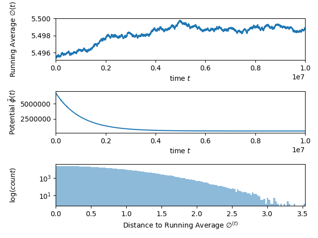 Figure 1
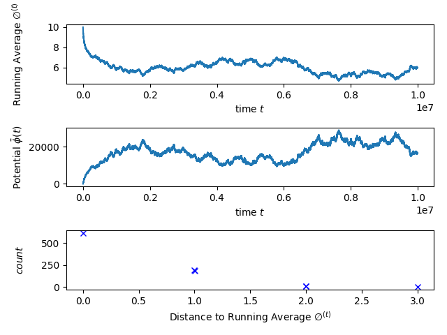 Figure 2
Peer Reviews
No public reviews on file for this paper yet. If you reviewed it on a platform where reviews are public (OpenReview, ICLR, NeurIPS, ICML), you can paste yours below so the community can read it here.
Videos
No videos yet. Explain this paper in a talk, walkthrough, or lecture? Add one.
\newaliascnt
lemmatheorem \aliascntresetthelemma
\newaliascntcorollarytheorem \aliascntresetthecorollary
\newaliascntdefinitiontheorem \aliascntresetthedefinition
\newaliascntremarktheorem \aliascntresettheremark
\newaliascntfacttheorem \aliascntresetthefact
\newaliascntconjecturetheorem \aliascntresettheconjecture
\newaliascntobservationtheorem \aliascntresettheobservation
\newaliascntassumptiontheorem \aliascntresettheassumption
\newaliascntassumptionstheorem \aliascntresettheassumptions
\newaliascntpropositiontheorem \aliascntresettheproposition
\newaliascntclaimtheorem \aliascntresettheclaim
Noidy Conmunixatipn: On the Convergence of the Averaging Population Protocol
Frederik Mallmann-Trenn
Department of Computer Science, Technion, Haifa, Israel
Yannic Maus
Dominik Pajak
Department of Computer Science, Technion, Haifa, Israel
Abstract
We study a process of averaging in a distributed system with noisy communication. Each of the agents in the system starts with some value and the goal of each agent is to compute the average of all the initial values. In each round, one pair of agents is drawn uniformly at random from the whole population, communicates with each other and each of these two agents updates their local value based on their own value and the received message. The communication is noisy and whenever an agent sends any value , the receiving agent receives , where is a zero-mean Gaussian random variable. The two quality measures of interest are (i) the total sum of squares , which measures the sum of square distances from the average load to the initial average and (ii) , measures the sum of square distances from the average load to the running average (average at time ).
It is known that the simple averaging protocol—in which an agent sends its current value and sets its new value to the average of the received value and its current value—converges eventually to a state where is small. It has been observed that , due to the noise, eventually diverges and previous research—mostly in control theory—has focused on showing eventual convergence w.r.t. the running average. We obtain the first probabilistic bounds on the convergence time of and precise bounds on the drift of that show that albeit eventually diverges, for a wide and interesting range of parameters, stays small for a number of rounds that is polynomial in the number of agents. Our results extend to the synchronous setting and settings where the agents are restricted to discrete values and perform rounding.
Frederik Mallmann-Trenn and Dominik Pajak were supported in part by NSF Award Numbers CCF-1461559, CCF-0939370, and CCF-18107. Yannic Maus was partly supported by ERC Grant No. 336495 (ACDC).
Contents
1 Introduction
We consider the problem of distributed averaging by a group of agents (e.g., sensors), initialized with values that represent, for example, different temperature measurements. The agents’ goal is to compute the average of all the initial values using the following simple dynamic: In each discrete round, two agents are drawn uniformly at random from the whole population, communicate their values to each other and set their new values to the average of their old value and the received value. Converging to the average plays a key-role in many applications, e.g., for sensor networks [58, 52], social insects [10], and robotics [21, 31]. In all of these applications, the agents (sensors, ants, and robots) are very simple and are therefore limited in both memory and communication. Moreover, communication is often erroneous.111Consult Section 1.1 for a more detailed review of these applications including the limitation of agents and further motivation. Section 1.1 also contains related work on the averaging protocol. This motivates the study of the aforementioned simple averaging dynamic in a setting where the agents only remember one value, do not use any additional memory, and the communication is subject to noise. We model the noise in the communication as follows: Whenever an agent sends any value , the receiving agent receives , where random variable is distributed according to some zero-mean probability distribution , e.g., a normal distribution. The agents update their values as follows: whenever two agents communicate, each agent sets its new value to the average of their old value and the received value; note that—due to the noise—the two agents might have distinct new values.
The values of the nodes in step of the process are denoted by . We consider the following models: (i) the sequential setting where one pair of agents is chosen uniformly at random and (ii) the synchronous setting where each agent is matched to exactly one other agent chosen uniformly at random. The two quality measures of the convergence used in this work are (i) the total sum of squares , where is the initial average and (ii) the sum of squared distances to the running average , where is the running average. Our contributions can be informally summarized as follows:
- (i)
We give, under mild assumptions on the noise, the first bounds on the convergence time of the running average in the noisy gossip-based communication setting. The bounds we obtain are—up to a constant factor—tight. In particular, the potential converges to a value that is linear in and the second moment of the noise ; which is tight. So far it was only known that the process eventually converges to a state where is small (e.g., [56]), but precise bounds were not known. (Theorem 1.1) 2. (ii)
We show that, in contrast to the current belief, one can hope to converge to the initial average in addition to convergence to the running average as long as the number of rounds are bounded: It was known that , due to the noise, eventually diverges (the running average diverges from the initial average) and for this reason related research—mostly in control theory—has focused on showing eventual convergence w.r.t. ; leaving aside. Since we give precise bounds on the convergence time of the running average, we can show the following. Under mild assumptions on the noise, converges to almost the same value as as long as the number of time steps is bounded by , where is the number of nodes. (Section 1.2) 3. (iii)
We pioneer in the discrete setting in which the agents can store only integer values and the noise is also an integer. In this setting the agents in our algorithm perform randomized rounding. We show that this only causes a negligible difference from the continuous case. (Section 1.2) 4. (iv)
We study both the sequential and the synchronous setting and show that there is no significant difference (up to a scaling of time) between the models. (Section 1.2) 5. (v)
We perform simulations in the setting where nodes are limited in storage, * i.e.,* they can only store values from a bounded range. This leads to a much faster (by order of magnitude) divergence between the running average and the initial average. Our simulations also seem to indicate strong bounds on the distribution of distances to the running average in our main model (unbounded values). (Section 5)
The convergence time of the averaging processes in the gossip-based communication setting without noise has been studied before (e.g., [39]). However, to the best of our knowledge, no bounds on the convergence time are known in the gossip-based communication setting with noise. We continue with a detailed motivation for studying noise in the simple averaging dynamic and related work.
1.1 Motivation and Related Work
Converging to the average plays a key role in many applications in which agents have limited computational and communication power, e.g.,
- (i)
sensor networks [58, 52]: here there is a wide range of application including terrain monitor applications [53], computing an average temperature, PIR sensors measuring the infrared light radiation emitted from objects, and many more applications. In such scenarios links are often faded [48, 14], 2. (ii)
social insects: for ants, values could represent the individuals’ different assessments of nest qualities when house hunting [10] or the deficit of workers at a given task [43], and 3. (iii)
robotics [21, 31] and in particular memory-limited robots, e.g., Kilobots exploring the percentage of white tiles in an area [22], or microbots measuring the concentration of chemicals.
In all of these applications the agents (representing sensors, ants or robots) are very simple and severely limited in both memory and communication. Moreover, the communication is often not only limited but also erroneous (e.g., consider wireless communication with obstacles between robots), or received messages are subject to interpretation (e.g., when insects communicate through gestures [41]). Motivated by this unreliable communication in applications we study the simple averaging dynamic where the communication is subject to noise.
We continue with related work. The problem of distributed values converging to the average (often without noise) has been studied in various areas reaching back to early versions studied in statistics [19, 27, 32]. However, to the best of our knowledge, none of the studied models match our model. We review the related work by areas:
-
average consensus and its applications,
-
gossip-based communication models,
-
consensus protocols in population protocols,
-
biological distributed algorithms,
-
noise and failures in sensor networks.
Average consensus and its applications
Consensus has been studied intensively in various settings in general network topologies, much of it under the name of average consensus [57, 55]. Most of this work is orthogonal to our work: First, due to the general network topology and the fact that, in each step of the studied algorithms, the agents update their values with a weighted average of all of their neighbors’ values whereas in our averaging dynamic, an agent can only access a single other value per interaction. Second, while the potential functions in these works and the noise, if any, are usually identically or similarly defined as in our work the main goal of these papers is—just as in the classic works—to study under which circumstances the processes eventually converge to a state with a small potential function [57], whereas we are interested in the number of interactions until our process obtains a small potential. Recent papers [47, 11, 42, 15] consider the convergence rate of the weighted averaging process, but only in the noiseless setting. Average consensus has also been studied in networks with time-varying topologies [46, 51]. Variants with noisy communication were studied [57, 38], but they only consider additive noise and assume it to be zero-mean with unit variance (as mentioned before, only convergence in the limit is shown). The noisy version of the problem also received ample attention in control theory [54, 50, 49]. Already in the early works on average consensus immediate applications of converging to the average were discovered and intensively studied, e.g., applications to load balancing between parallel machines [9, 18] or to coordinate distributed mobile agents [9, 36, 24]. For a more detailed overview on average linear consensus consult the survey [28].
Gossip-based communication models
Much closer to our work is the study of aggregating information in gossip-based model. In this model, each node can contact one of its neighbors in the network in each round and exchange information with it. Even though a node can be contacted by many neighbors in a single round, this model, if applied to the complete graph, is very similar to our synchronous model. On the complete graph [39] shows that interactions are enough to approximate the average well with high probability. On the one hand they consider more general graphs (in some sense we consider the complete graph); on the other hand they do not consider noise, which simplifies their analysis of the convergence time significantly.
Consensus protocols in population protocols, biological distributed algorithms
Motivated by biological applications, population protocols have also been studied in the noisy setting in the context of biological distributed algorithms. The authors of [25] study rumor spreading and consensus in extremely faulty networks where a bit in a message can be flipped with probability . This was later generalized in [26] to plurality consensus. The authors of [8] study the differences between pull and push rumor spreading in the noisy setting. Reaching consensus to an opinion in population protocols in the noiseless setting has received much attention (see e.g., [4, 23, 1, 2, 5, 6, 20, 7, 40, 30, 29, 37]).
Noise and failures in sensor networks
The problem of converging to the average (and similar problems) have also been studied in (noisy) sensor networks [58, 52] where nodes again can interact with all their neighbors. In these networks another type of unreliable communication, i.e., packages might be dropped, has received ample attention, e.g., [12] studies the broadcast problem and [13] develops a framework to transform certain algorithms for failure free networks to also work in faulty sensor networks.
An interesting type of failure has been studied in [33]. There failures do not happen during the communication but the algorithm itself might be faulty, i.e., a state machine run at an agent might switch to a wrong state.
1.2 Formal Results
We now formally state our main theorems. For the ease of presentation, in the discussion we assume that noise is normally distributed with unit variance, , but our results hold for general variance . Let be the initial potential. Our first theorem shows that the agents converge to a small value of after parallel time222Recall that in parallel time we scale time by a factor of for a fair comparison with the synchronous time model. that is logarithmic in . In particular, if we use to denote the initial imbalance (), then it takes parallel steps for the potential to become . Note that means that the ‘average’ difference between the values of any two agents is constant and we show that the constant hidden in the -notation is actually very small. It is worth mentioning that this is tight in two senses: (i) In expectancy we have for any fixed time step , (i.e., after one parallel time step). Even in the case where all nodes initially have the same value, our results show that the potential increases after interactions in expectation by . (ii) At least parallel time steps are required333For the case where constant fraction of the values are at distance . to decrease the potential to , since the potential only drops in expectation by a constant factor in each parallel step. The formal statement is as follows.
Theorem 1.1** (Convergence to Running Avg.).**
Consider any noise-distribution with (at least) exponential-decay444In fact we only require the function to be smooth, which we define later. This class is much broader and contains most of the famous distributions including the normal distribution, geometric distribution and the Poisson distribution. . Fix any . Let be large enough. The following hold:
- (i)
for any with probability at least we have , 2. (ii)
for any (parallel time) with constant probability we have and 3. (iii)
even without noise, for any we have .
While the above theorem shows a quick convergence to the running average, this does not imply convergence to the initial average. In fact, as time progresses the distance to the initial average () is likely to increase. Nonetheless, in the case of the Gaussian white noise model we can bound the drift of the running average from the initial average in a time window of steps (cf. Section 4). Theorem 1.1 roughly says that after at least steps the distance to the running average is small if we start with a potential that is polynomial in . Thus, as long as and we obtain . After the step time window the potential starts to increase again, which, is unavoidable, due to the noise causing drift of the running average; in Gaussian white noise model, the running average after steps diverges with constant probability from the initial average by (Section 4). This in turn implies that .
Corollary \thecorollary ((Bounded) Divergence from Initial Avg.).
In the case of Gaussian white noise model, for any and large enough and all we have
- (i)
‘non-divergence for steps’, i.e., with probability at least and 2. (ii)
‘divergence for steps’, i.e., with constant probability.
If one can bound the divergence between the running average and the initial average for a general noise-distribution with (at least) exponential-decay555Again, we only require the function to be smooth, which we define in Section 3. the following remark is useful to obtain a similar bound for the as in Section 1.2.
Recall that and in particular, denotes the initial average.
Remark \theremark.
Fix any . Let be large enough. For any fixed with probability at least we have .
Section 1.2 follows by rewriting (cf. Section 2) and plugging in the first part of Theorem 1.1. Section 1.2 then follows by plugging in the bounded deviation of the running average from the initial average for the Gaussian white noise model (cf. Section 4).
The Influence of Rounding
Agents with limited computational power might not be able to store real values. Motivated by this we also consider the setting where agents can only store integers. In particular, we consider the case that the averaging protocol is augmented with the following rounding procedure: Assume that the noise takes only integer variables. After a node receives the value from node , the node averages it as before and then rounds up or down with equal probability. In Appendix D we show how to relate the setting of rounding to the original setting allowing us to derive the following corollary.
Corollary \thecorollary.
The bounds of Theorem 1.1 and Section 1.2 hold even if rounding is used.
The Synchronous Model
In Appendix C, we show how our results extend to the synchronous setting. It turns out that the results are the same up to a rescaling of time.
Corollary \thecorollary (Synchronous Setting).
The bounds of Theorem 1.1 and Section 1.2 hold even in the synchronous setting, where time is rescaled by a factor of .
Experimental Results
In Section 5, we simulate the averaging dynamic in various settings. In the first setting, we consider the distribution of the distances between agents’ values and the running average. Our simulations show that these distances seem to follow an exponential law, i.e., the concentration is even stronger than what Theorem 1.1 implies.
Due to the limited memory of agents it would be desirable to obtain similar results as in Theorem 1.1 for the averaging dynamic in the setting where agents can only store values from a bounded range. However, our simulations in Section 5 show that this setting leads to a much faster (by order of magnitude) divergence between the running average and the initial average.
1.3 Technical Contributions
While it is not hard to show that in expectation the potentials and decrease in one step as long as their value is large, it is surprisingly challenging to derive probabilistic bounds on either potential at an arbitrary point in time, * i.e.,* bounds of the type . Two of the reasons are as follows. (i) The potential decreases (expectedly) only conditioned on the fact that it is large enough. In fact, when the potential is small, then due to the noise it will increase in expectation. (ii) Since we study general distributions and in particular the normal distribution, the noise in a given round can be arbitrarily large leading to an arbitrarily large increase in ; if the protocol runs long enough (possibly exponentially long in ) we, indeed, will have encountered some time steps with a very large potential increase. There are surprisingly few analytical tools for using potentials as with challenges (i) and (ii). One notable exception is Hajek’s theorem [34], which can be used to bound the value of such a potential at a given time . However, in our setting—with our potential function—the results obtained are very weak.666Hajek’s theorem considers the moment generating function of the potential. In order to apply the theorem to our potential, it seems that one would need to consider a logarithmic version of the potential, which together with the moment generating function results in bound that is weaker than a simple union bound.
Instead, we use a more sophisticated approach that at its core has a decomposition of the potential change in a single time step into three additive (but dependent) random variables. We iterate this decomposition over time throughout some interval and sum the respective variables which we will denote as , , and . Then (cf. Section 3) we are able to bound the potential change at the end of the interval as
[TABLE]
Due to the dependencies between the three variables we use strong Martingale concentration bounds to separately upper bound and lower bound (cf. Section 3). We then use union bound—to circumvent the dependencies—to bound each of these variables allowing us to get a bound on Equation 1. It is critical that we define the random variable in such a way that it always has an expected decrease. This is in stark contrast to the entire potential, which, as we mentioned before in (i), only decreases in expectation when it is large. Having an unconditional decrease of allows us to consider arbitrarily large intervals. With these bounds at hand one can use Equation 1 to obtain probabilistic bounds on the potential at any given point time . However, due to the bound on the total bound becomes very weak for large intervals. As a remedy, we carefully trace the change in the potential in different regimes (with several phases in each regime) and we separately apply the aforementioned analysis with a fresh (small) interval in each phase. The intervals (and thus also the phases) have variable length—decreasing geometrically or even exponentially, depending on the regime.
2 Model
In this section we present the model including all assumptions. We have a collection of agents that have initial values . Time is discrete and denotes the value of agent at time . Recall that denotes the average value at time ; in particular, denotes the initial average. For two random variables and we write if they have the same (probability) distribution. Next, we define the communication models.
Definition \thedefinition (Communication Models).
We consider two communication models.
- (i)
Sequential model*: At every discrete time step two of the agents are chosen uniformly at random (with replacement777This is not crucial to our results, but simplifies the calculations slightly.) and exchange their current values and , where the values received are and , where .* 2. (ii)
Synchronous model*: At every discrete time step a perfect matching is chosen u.a.r. among all perfect matchings on the agents.888Again, we allow matchings of the kind for simplicity. It is easy but slightly less aesthetic to modify our results to exclude matchings . * All matched agents interchange their values as in the sequential model. 3. (iii)
Sequential model*: At every discrete time step two of the agents are chosen uniformly at random (with replacement999This is not crucial to our results, but simplifies the calculations slightly.) and send their current values and to each other, where the values received are and , where .* 4. (iv)
Synchronous model*: At every discrete time step a perfect matching is chosen u.a.r. among all perfect matchings on the agents*101010Again, we allow matchings of the kind for simplicity. It is easy but slightly less aesthetic to modify our results to exclude matchings . . All matched agents interchange their values as in the sequential model.
We use the parallel time, which was first defined in [3], to denote the time step in the sequential model. This notion eases the comparison of results in both models, as the total number of interactions is up to a factor of equal.
Definition \thedefinition (Noise Models).
Let be the value sent by an agent. The value received is , where is distributed according to some zero-mean noise distribution and let .
We consider general noise distributions and our results depend on the moments of . The following two models are of special interest in this paper.
- (i)
Gaussian white noise model where for an arbitrary . 2. (ii)
Discrete white noise model where , with , for and , where . Note that .
From now on we assume that the noise is distributed according to a fixed noise distribution that is independent of .
Definition \thedefinition (Averaging Dynamic).
We consider the real valued and the discrete valued algorithm. A node with value at time receiving the input sets its new value to
- (i)
* in the real valued model.* 2. (ii)
v^{\prime}=\begin{cases}\left\lceil\nicefrac{{(v+w)}}{{2}}\right\rceil&\text{ w.p. \frac{1}{2}}\\ \left\lfloor\nicefrac{{(v+w)}}{{2}}\right\rfloor&\text{ otherwise}\end{cases}* in the discrete valued model.*
A probability distribution is called sub-Gaussian if for we have that there exists positive constants such that for every we have
Whenever we calculate the new values by conditioning on the current state, we use small letters to denote fixed values and capitalized letters to denote random variables. Furthermore, we use bold-face to denote vectors. Throughout the paper we will assume that the number of agents is large enough and in particular
We define the following potentials which are essential in all our proofs and formal results.
Definition \thedefinition (Potentials).
[TABLE]
When clear from the context we drop the time index and we write instead of , instead of , etc. Similarly we will use the following short forms and . We emphasize that the difference between and is that the former measures the squared distance w.r.t. the running average and the latter w.r.t. initial average. Initially, we have . The following fact shows how relates to and how relates to .
Fact \thefact.
We have that
- (i)
* and* 2. (ii)
**
Proof.
Consider part .
[TABLE]
∎
Consider part .
[TABLE]
Note that many alternative ways to define the potential at a time such as the max distance and norm give only a very partial picture: The max distance to the mean for example does not distinguish between just one node being far and all nodes being far. On the other hand, the norm does not does not ‘punish’ outliers enough: there is no difference between nodes being off by from the average and one node being off by .
Notation
We use to denote that is distributed according to probability distribution . For two random variables and we write if is stochastically dominated by , i.e., for all . We use to denote the -norm. In the sequential model we have two random variables and for the noise of the channel at time step (recall that and are distributed according to ). We define the following two random variables and that will play a key-role in our analysis:
[TABLE]
Fact \thefact.
In the Gaussian noise model, we have and , where denotes the gamma distribution.
When clear from the context we simply write and instead of and , respectively. We use to denote the filtration at time , which encapsulates all randomness up to time as well as the initial values of the nodes; hence it defines the state at time completely.
3 The Sequential Setting: Convergence towards the Running Average
Conditioning on all the randomness until time , * i.e.,* conditioning on , we define
\Delta^{(t+1)}=\begin{cases}\frac{\left(x_{i}^{(t)}-x_{j}^{(t)}\right)^{2}}{2\bar{\phi}(\mathbf{x}^{(t)})}&\text{ for \bar{\phi}(\mathbf{x}^{(t)})>0}\\ 1/n&\text{ otherwise }\end{cases}, where and are the chosen in round .
Lemma \thelemma (One Step Bound).
Fix an arbitrary potential at time . Suppose the pair was chosen to communicate and condition on the filtration (all events that happened up to round ). Then, the following holds
[TABLE]
Further we have .
In order to prove the statement, we first calculate the exact expected change in one step (Section B.1). We then majorize (stochastic dominance) with the slightly more convenient statement above.
For an arbitrary time interval define
[TABLE]
Note that, in the definition of , we sum up over all time steps in the interval and we consider the pair and that is chosen in round (in each round a different pair and can be chosen). With Section 3 and the definitions of and we can deduce the following decomposed bound on the potential for an arbitrary interval.
Proposition \theproposition (Decomposition of Potential).
Fix arbitrary and consider the interval . For we have that
[TABLE]
In the following we define smooth noise distributions. Define
[TABLE]
Using strong martingale concentration bounds (Theorem A.3 and Theorem A.4) and bounding the variance, we deduce the following upper bound on and lower bound on .
Lemma \thelemma.
Let be such that and consider the interval .
- (i)
With probability we have
[TABLE] 2. (ii)
For any , w.p. at least we have
Our main results only hold for smooth noise distributions, which we define in the following.
Definition \thedefinition.
A noise distribution is smooth if for all and all we have .
However, note that any (sub-)linear probability distribution and even some inverse polynomial distributions are smooth. Thus many practically relevant distributions such as Gaussian, binomial and Poisson distributions are smooth. For example, for the standard normal distribution () we have , since in each time step the probability that the exceeds is equal to the probability that exceeds which happens w.p. at most . Taking union bound over all steps shows that it is smooth.
For smooth noise distributions we can upper bound the additive increase due to the noise.
The following proposition almost directly implies Theorem 1.1.
Proposition \theproposition.
Fix any and assume that the noise distribution is smooth. There exists a constant such that for a time step with potential we have
[TABLE]
where and
Proof Sketch.
We only sketch the proof idea for a simplified setting; during the sketch we assume that (with ) and also that is at least . The main ingredients for the proof are Section 3 and Section 3. For an interval Section 3 upper bounds the potential at time by
[TABLE]
where is the length of the interval. Section 3 lower bounds and upper bounds the sum . To prove Section 3 we have to show that the initial potential decreases to after time steps with probability . Optimally, we would use a single application of Section 3 to upper bound the potential as in Equation 2 and then bound the terms and via Section 3. However, the bounds on and given by Section 3 are too loose to yield the desired result via a single application of Section 3 and Section 3 with the whole time interval . For example, the bound on inherently has a term of order , where is the potential at the start of the interval for which Section 3, (i) is applied. Thus a one shot proof as described above can never reach a potential below . This is not sufficient if the initial potential is large, e.g., say for .
To circumvent this problem we apply Section 3 and Section 3 several times for smaller time intervals: More detailed, we split the proof of Section 3 into two regimes. In regime we use several phases to decrease the potential to . If the potential is at the beginning of a phase a single application of Section 3 and Section 3 reduces the potential to . The length of each such phase is geometrically decreasing by a factor where the first phase is of length . After the last phase of regime the potential is of order .
Then, in regime the potential reduces from to , again through several phases. If the first phase of regime 1 starts with a potential of size , the phase has length . If there was no additive increase due to the noise, then this would reduce the potential to [math]. However, there is an additive increase of which leaves us with a potential of size . The next phase will therefore be of length etc. This is repeated for phases until the potential reduces to , which, as we explained in Section 1.2, is the furthest the potential can be decreased .
Putting everything together, we get that after rounds the potential reduces to . ∎
The full proof of Section 3 handles general and general and thus it is significantly more technical. It can be found in Section B.3. From Section 3 we are able to derive Theorem 1.1, whose proof can be found in the appendix.
4 Deviation from the Initial Average
An informal argument for the statements in this section in the special case of can be found in [56]. Before we state our results we need the following result on the standard normal distribution.
Theorem 4.1** ([17]).**
Let denote the cumulative distribution function of the standard normal distribution. We have for :
[TABLE]
We can now state and prove the main results of this section.
Lemma \thelemma.
For any and any , we have with probability at least , where is the noise of the channel. In particular, for the Gaussian white noise model setting where we have . Thus
- (i)
|\varnothing^{(t)}-\varnothing^{(0)}|\leq\frac{\sigma\sqrt{t\ln(1/\delta)}}{n}\text{ w.p. at least 1-\delta}** 2. (ii)
|\varnothing^{(t)}-\varnothing^{(0)}|\geq\frac{\sigma\sqrt{t\ln(1/\delta)}}{n}\text{ w.p. at least \frac{\delta}{2\sqrt{2\ln(1/\delta)}}.}**
Proof.
Note that , where and are the nodes scheduled in the current round and . Applying this recursively and using that all follow the same distribution we have . Using that completes the proof of the first part.
Consider . For a general normal distribution with mean and variance we have that
[TABLE]
where denotes the cumulative density function of the standard normal distribution. Applying the upper bound of Theorem 4.1 and using symmetry of the normal distribution, it holds for , and that
[TABLE]
Taking Union bound yields the claim.
Consider . By applying the lower bound of Theorem 4.1 and using similar arguments as before, we have for , , and
[TABLE]
Using the Berry-Esseen theorem, one can easily prove similar bounds for any distribution with bounded third moment including discrete white noise. Similarly, rounding can easily be taken care of by applying the ideas from Appendix D.
In the following we consider the potential as a Martingale allowing us to use Theorem A.3 to derive the desired concentration bounds. The following bound is weaker than the aforementioned bounds, however, it is useful whenever the noise is such that is small.
Proposition \theproposition.
For any and any we have with probability at least .
Proof.
We start by showing that the sum of entries is a Martingale
[TABLE]
By law of total expectation, summing over all choices of and , we get that is a Martingale.
Since is a Martingale, so is , where we used that . Note that
[TABLE]
w.p. at least per time step and hence, by Union bond, w.p. at least throughout the interval. By Theorem A.3, with , , and we get
[TABLE]
Taking Union bound yields the r.h.s. inequality of the claim The l.h.s. follows by using Theorem A.4 instead of Theorem A.3. ∎
5 Experimental Results
The goal of this section is twofold. First, we seek to better understand the distribution of the distances . Second, we simulate a setting in which the range of values is bounded motivated by computational and storage limited agents. All results in this section are based on an implementation of the simple averaging dynamic. The code (python3) for the experiments can be found here [44].
5.1 The Distribution of the Distances
The experiments suggest that the distance decays at least exponentially. Note that the experiments only show a single iteration, however, this phenomena was observable in every single run. The bound on we obtained in Theorem 1.1 only implies that is at most . However, we conjecture, for sub-Gaussian noise that (cf. 1(a)). Showing this rigorously is challenging due to the dependencies among the values. Nonetheless, such bounds are very important since they immediately bound the maximum difference and we consider this the most important open question.
5.2 The Bounded Values Setting
One of the motivations for the very simple averaging dynamic arises in the setting of limited computational power of the interacting agents. So far we assumed that agents can store and transmit (intermediate) values from an unbounded range. For many applications and in particular motivated by agents with bounded memory one would hope for similar results if there is a maximum and a minimum value that can be stored or transmitted. The formal definition is as follows: values can only be from the range ( in our experiments). We assume noise of the channel cannot produce values larger than or smaller than , which can be motivated as follows in the setting where the values correspond to amplitudes: here and are simply the amplitudes (high amplitude and no amplitude) where the signal-to-noise ratio is very large, and noise becomes negligible. An equivalent model is that the agents know the range of possible communication values, and hence, they can simply correct every value larger than to . In particular when agents only have limited storage, the communication range will often be bounded, and even rounding might become necessary (see Appendix D).
We refer to these equivalent models as the model with cutoffs. While the experiments indicate that values still converge towards the running average, there is a clear drift of the running average from the initial average if the input values are chosen unsuitably. In our experiments, we set the range of values to , use the noise described in the discrete noise model together with rounding. Initially, all agents have value . We see a drastic drift of the running average (see 1(b)). Even though the initial average is , the running average appears to approach the midpoint of the range, i.e., 5. The histogram of distances to the initial average shows even more clearly that the values are not concentrated around the initial average. Although the experiments only show a single iteration, this phenomena was observable in every single run. We believe that the reason for this is simply that the noise is no longer symmetric and no longer zero-mean due to the cutoffs . Proving convergence to the running-average in this model seems challenging and interesting.
We believe that the insights in bounding this potential might be useful in similar problems.
6 Conclusion and Open Problems
In this paper we showed bounds on the convergence time for the unbounded setting. Our simulations in Section 5 yield two interesting open problems: (i) study the setting where the values are restricted to some interval (in this case the noise is no longer symmetrical) and (ii) prove tail bounds on the distance distribution w.r.t. to the running or initial average. Another interesting research direction is to move away from zero-mean noise and consider biased noise models: how quickly can the bias(es) be estimated and is convergence still feasible by compensating for the (learned) bias?
Appendix A Auxiliary Claims
Theorem A.1** (Weierstrass Product Inequality).**
We have
- (i)
[TABLE]
if and either for all or for all . 2. (ii)
[TABLE]
if , and for all .
Proof.
Consider which trivially holds for . Now consider . Taking the logarithm on both sides and treating the as probabilities, where we introduce a dummy element with , and derive
[TABLE]
Where we used Jensen’s inequality. This concludes the proof.
∎
Proposition \theproposition (Distribution Facts).
Let . We have
- (i)
** 2. (ii)
.
Proof.
First observe that , where is the chi-squared distribution with degree of freedom. Hence, and implying and . ∎
We will make use of a slightly generalized version of the Hoeffding bound (see [35]).
Theorem A.2** ([35]).**
Let be a sum of independent random variables with for all . Then
[TABLE]
The following Theorem finds its origins in the work of [45].
Theorem A.3** ([16, Theorem 6.1]).**
Let be the martingale associated with a filter satisfying
- (i)
, for ; 2. (ii)
, for .
Then we have
[TABLE]
Theorem A.4** ([16, Theorem 6.5]).**
Let be the martingale associated with a filter satisfying
- (i)
, for ; 2. (ii)
, for .
Then we have
[TABLE]
Throughout this paper we will frequently make use of the fact that the sum of independent variables is a martingale.
Appendix B Missing Proofs: Sequential Setting (Section 3)
B.1 Sequential Setting: One Step Potential Change
In the following we bound the one step potential change.
Lemma \thelemma.
Fix an arbitrary potential at time . Suppose the pair was chosen to communicate and that the coins have been flipped to determine the noise, i.e., and . Then,
[TABLE]
Proof.
In order to bound we will make use of Section 2 and analyze , which is slightly more convenient, since we do not need to compute the change of .
Note that besides node and node no other nodes will change their value. However, the contribution of each agent to the potential might change. Consider for
[TABLE]
The same holds if we substitute with and thus, for agent the change in the contribution to the potential equals:
[TABLE]
We get that if in step an interaction between and happens, and that the change of the potential is as follows:
[TABLE]
[TABLE]
By Section 2 and via dividing the equation by we obtain:
[TABLE]
Recall, that by definition (see Section 2) and where and are the random variables that determine the noise of the communication in time step . Conditioning on all the randomness that has happened until time , * i.e.,* conditioning on , we define the as follows:
\Delta^{(t+1)}=\begin{cases}\frac{\left(x_{i}^{(t)}-x_{j}^{(t)}\right)^{2}}{2\bar{\phi}(\mathbf{x}^{(t)})}&\text{ for \bar{\phi}(\mathbf{x}^{(t)})>0}\\ 1/n&\text{ otherwise }\end{cases}, where and are the chosen agents in round .
Using the above, we can prove the following two statements.
Proof of Section 3.
The first result follows with the definition of and and with Section B.1.
Note that the term is always negative.Hence, by Section B.1, we get that for fixed and
[TABLE]
W.l.o.g. assume ; otherwise the claim follows trivially (by definition of ). Taking the expectation over all choices of and :
[TABLE]
Note that in the Gaussian noise model, all follow the same law . Thus, using that the sum of two Gaussian with law are distributed , we obtain . Finally, the sum of two squared Gaussians each with distribution we have .
∎
For an arbitrary time interval define
[TABLE]
Note that and in the definition of also depend on and are the nodes (we use nodes and agents interchangeably) that are chosen in that round.
Proof of Section 3.
The potential is maximized, if all decreases happen at the beginning and all increases happen in the last time step.
In order to analyze the decrease due to we will make use of the Weierstrass Product Inequality (Theorem A.1) to derive
[TABLE]
B.2 Bounding , , and
In this section we bound the terms of Section 3 separately. Therefore, for any , any and any we define the following values:
[TABLE]
We want to emphasize that these values are not random variables and their values are not related to the actual outcome of the randomness during a run of the protocol. In words (, respectively) denotes the maximum value that is reached w.p. at most by and during the interval , respectively. Note, that the value of and is independent from the choice of as the noise at different time steps is independent. We will assume throughout the proofs; we will only consider that are a function of and hence we restrict ourselves to noise functions that grow with .
From now on and throughout the proof assume that is fixed and we continue with upper bounding .
Lemma \thelemma.
Fix arbitrary , consider the interval and let be the value as defined in Equation 7 where . Then, w.p. at least we have
[TABLE]
Proof.
By definition w.p. at least for every we have . Assume that this property holds throughout interval .
Define and note that \big{(}X_{t^{\prime}}\big{)}_{t_{0}<t^{\prime}\leq t_{1}} is a martingale. We obtain that and . Let . We have that
[TABLE]
and apply Theorem A.3 to the martingale which yields
[TABLE]
Taking a union bound with the case that is not smaller than for some , yields the claim. ∎
In the following we bound the first, second moment of and its maximum possible value; we use this result in the proof of Section B.2.
Fact \thefact.
Fix . In particular, this fixes the vector of values and . Define the following random variable , where and are chosen uniformly at random. We have:
- (i)
** 2. (ii)
** 3. (iii)
**
Proof.
Recall that we allow . Using this, we derive
[TABLE]
Moreover, using that , we get
[TABLE]
The third claim is true because for any we have
[TABLE]
We continue with upper bounding .
Lemma \thelemma.
Fix arbitrary , consider the interval and let be the value as defined in Equation 9 with . Then, w.p. at least , we have
[TABLE]
Proof.
By the definition of (see Equation 4) we have w.p. throughout . Further by Section B.2 with probability we have for all . We assume that both properties hold (the case that they do not hold is submerged in a union bound (that leads to a probability ) with all other undesirable cases).
Recall the definition as in Section B.2 and note that for , we have . For each such the sequence \big{(}S^{*}((t_{0},\tau])\big{)}_{t_{0}\leq\tau\leq t^{\prime}} is a martingale and the goal is to apply Theorem A.3 to it.
We assume a process in which for all , where is defined as in (8). In this process we will bound the size of . Using this bound, we show that the original process and never diverge (with large probability) and hence the bound on we obtained in carries over to .
Consider . Using that the potential is at most and Section B.2, we get a bound of on the second moment of (conditioned on ). Using this bound and since and are independent and as and equal [math] we obtain that
[TABLE]
Define . As the potential is never above we obtain for all due to Section B.2, (iii). Due to the definition of this implies that
[TABLE]
throughout the interval .
The bound on the variance and Equation 10 are sufficient to apply Theorem A.3 and we obtain
[TABLE]
where we used that . Let and . Then we have which yields
[TABLE]
To prove the equivalence between the processes, we need to show that the potential at step does not exceed ; in this proof we use and . The first statement holds with probability as we just showed and we assumed to hold throughout the whole proof at the very beginning. Thus we obtain
[TABLE]
where the last inequality follows as for all .
The last induction step shows . This combined with a union bound about the error probabilities from the two assumptions at the start of the lemma ( each) yield that the result holds with probability . ∎
Now, we lower bound which is essential to obtain progress through Section 3.
Proof of Section 3, (ii).
Let . Note that . By Section 3, we have and , where Why follows since implies that each element of the sum is smaller. By Theorem A.4 with for all , with , we get
[TABLE]
Proof of Section 3 (i).
In order to derive the result, we the bound on (Section B.2) and on (Section B.2). Section B.2 applied with and for and large enough with probability yields:
Roughly upper bounding the terms yields
[TABLE]
Furthermore, we have, by the definition of (Equation 8),
[TABLE]
where we used that . Note that . Thus, putting everything together yields
[TABLE]
Applying Section B.2 with yields that with probability we have
[TABLE]
Combining the bound on and yields the claim with probability .
∎
B.3 Proof of Section 3 and Theorem 1.1
In the section we prove Section 3. A proof sketch can be found in Section 3. Using Section 3 and Section 3 our main theorem Theorem 1.1 follows almost immediately.
Proof of Section 3.
We distinguish between regimes based on the value of for thresholds that we define later. We have two regimes: regime starts at time and ends when the potential is below a threshold which marks the start of regime ; note that in order to simplify indices in the calculations, we define regimes and phases (within the regimes) backwards, starting with large numbers and then reduce. We divide each regime into phases. The phases of regime are such that the ’th phase starts when . Phases in regime are also counted backwards starting from phase until we reach phase [math]. We use , to denote the start of the ’th phase of regime . Where the first phase is
Let , . We define the boundaries and (which will be used to guide the potential decrease) as follows. Let be a large enough constant and .
[TABLE]
[TABLE]
Regime 2
Consider phase , that is, the potential at the start of the phase is in the interval . Let .
In the following we bound the increase due to after steps. By Section 3, (i), after time steps we have that each of the following bound holds w.p. at least .
[TABLE]
In the following we bound the terms of (12). First we obtain
[TABLE]
Here, follows because for large enough and follows because .
We continue by bounding the terms in front of the square-root of (12). To do so we consider the factors separately. Due to and for large enough we have
[TABLE]
Due to the smoothness of the noise distribution, we have
[TABLE]
Moreover, again using for , we can bound
[TABLE]
Putting everything together, using that .
[TABLE]
where follows because for large enough .
Plugging (B.3) and (B.3) into (12) yields
[TABLE]
Finally, by Section 3, (ii) , and since we have
[TABLE]
By Section 3, Section B.3 and Equation 16 we obtain
[TABLE]
The number of time steps of all phases in regime form a geometric series and is dominated by the length of the first phase, that is, regime takes at most
[TABLE]
time steps. The probability of success of each phase also forms a geometric series and by a union bound over all phases, the probability of failure is .
Regime 1
. Here we define the phases informally to avoid an overload of notation involving the tower-function. Instead of reducing to as in a phase in the regime above, here, in a single phase, we reduce the potentital from to and then from to etc., where is such that this recursion forms a geometric series. We stop once the potential is smaller than .
From now on fix a phase in regime and assume that the potential is of value at the start of the phase. Let , where is some large enough constant. If the length of a phase is and once is close to the length of a phase is , more formally the length of a phase is . By Section 3, (i), after time steps we have,
[TABLE]
In the following we bound the second term of (17). Since we are in regime we have and we can deduce that and . We obtain
[TABLE]
To upper bound this term by we observe that the polynomial appearance of is in and only in the term . All other terms do not ruin the claim and we can bound (18) by . Thus,
[TABLE]
By Section 3 and using the lower bound on from Section 3, (ii) we obtain
[TABLE]
Now there are two cases. If , then and we continue with the next phase. On the other hand, if , then we have and we are done.
We now calculate the success probability as well as total length of regime . In the last run we set the error parameter to . In the ’th run before the last run the error parameter is set to . Clearly, the total error sums up to at most . Thus with probability of at least the potential decreases to .
To analyze the runtime of regime first consider the case that regime is executed before regime because the initial potential was larger than . Then we have phases and the longest phase has length . Thus one can immediately bound the runtime of regime as . As the length of the phases—ignoring the factor of — is decreasing more than geometrically a tighter analysis shows that the runtime of all phases can be bounded by . In the other case that regime is not executed before regime the initial potential is smaller than and we can replace all occurrences of in the runtime analysis with .
Combining Regimes and Phases
Taking a union bound over all errors in all phases in both regimes gives an error probability of at most . Note that regime 1 takes at most rounds. If regime 2 is necessary than and hence we can bound the number of rounds in regime 1 by
[TABLE]
Summing over both regime gives yields the claim. ∎
We are ready to prove the first main theorem.
Proof of Theorem 1.1.
Proof of (i). First observe that if and were to coincide with time as in Section 3 then the proposition immediately yields the result. Otherwise we apply Section 3 with an initial potential that is larger than . is chosen such that in Section 3 equals the in Theorem 1.1. Choosing a larger potential than the actual analysis does not harm the correctness of Section 3 as the proof does not consider an exact potential but always just upper bound on the potential.
Proof of (iii). The lower bound on the expected size () follows from the following argument. By Section B.1, summing over all pairs of nodes, we get
[TABLE]
Taking expectations on both sides and applying this recursively implies . Thus choosing yields .
Proof of (ii). Fix an arbitrary potential at round and consider the next iterations. W.l.o.g. there has to be a constant fraction of the nodes with a value of greater or equal to the running average at time ; otherwise there has to be such a fraction of nodes that have a value strictly smaller than the running average, in which case the proof is symmetric. Let be the set of these nodes. Order the nodes of according to their value in decreasing order (ties broken arbitrarily). Assign the first to and the remaining nodes to . There will be w.h.p. a set , of linear size in of nodes of that are chosen exactly once to exchange with another node of during the last steps and these nodes were not part of any other exchanges during the last steps. Now consider the exchange of two nodes that belong to : the node with the initially lower value, will after averaging have with constant probability a value that is by larger than before. Similarly, consider the exchange of two nodes that belong to : the node with the initially higher value, will after averaging have with constant probability a value that is by smaller than before.
Hence, by definition of the running average, irrespective of value of the running average at time , the potential is of size (due to the nodes of or due to the nodes of ).
∎
Appendix C Synchronous Model
In this section we consider the synchronous model and show that it is up to scaling of a factor of almost the same. In order to avoid confusion, we introduce for every variable in the sequential model the synchronous/parallel counterpart to emphasize the different model and the slightly different notation. The following two lemmas are the counterparts of Section 3 and Section 3. These two lemmas encapsulate the essential difference between both models.
Lemma \thelemma (Synchronous Setting).
There exists random variables , , and s.t.
[TABLE]
where
[TABLE]
In particular, in the Gaussian noise model, we have and , where denotes the gamma distribution.
This follows almost immediately from the sequential counter-part. In order to calculate the expectation, we can simply use linearity of expectation and multiply the sequential bound by a factor
Proposition \theproposition (Synchronous Setting).
*Consider the interval . Let ,
let and let . We have that*
[TABLE]
The rest of the analysis is a straight-forward adaption of the sequential setting with time being scaled by a factor of .
Appendix D The Influence of Rounding
The rounding can be implemented as follows assuming that the noise takes only integer variables. After a node receives the value from node , the node averages it as before and then rounds up or down with equal probability. In symbols,
[TABLE]
where is the integer valued channel noise. Equivalently, we can write
[TABLE]
where is the random variable satisfying
[TABLE]
Regardless of the current state, it holds that and . Thus we obtain that . If we substitute with in all proofs we obtain essentially the same results; the variance in the statements only increases by .
The reference list from the paper itself. Each links out to its DOI / PubMed record.
- 1[1] Dan Alistarh, James Aspnes, David Eisenstat, Rati Gelashvili, and Ronald L. Rivest. Time-space trade-offs in population protocols. In Proceedings of the Twenty-Eighth Annual ACM-SIAM Symposium on Discrete Algorithms, SODA 2017, Barcelona, Spain, Hotel Porta Fira, January 16-19 , pages 2560–2579, 2017. URL: https://doi.org/10.1137/1.9781611974782.169 , doi:10.1137/1.9781611974782.169 . · doi ↗
- 2[2] Dan Alistarh, James Aspnes, and Rati Gelashvili. Space-optimal majority in population protocols. Co RR , abs/1704.04947, 2017. URL: http://arxiv.org/abs/1704.04947 , ar Xiv:1704.04947 .
- 3[3] Dan Alistarh, Rati Gelashvili, and Milan Vojnović. Fast and exact majority in population protocols. In Proceedings of the 2015 ACM Symposium on Principles of Distributed Computing , PODC ’15, pages 47–56, New York, NY, USA, 2015. ACM. URL: http://doi.acm.org/10.1145/2767386.2767429 , doi:10.1145/2767386.2767429 . · doi ↗
- 4[4] Dana Angluin, James Aspnes, Zoë Diamadi, Michael J. Fischer, and René Peralta. Computation in networks of passively mobile finite-state sensors. Distributed Computing , 18(4):235–253, 2006. URL: https://doi.org/10.1007/s 00446-005-0138-3 , doi:10.1007/s 00446-005-0138-3 . · doi ↗
- 5[5] Luca Becchetti, Andrea E. F. Clementi, Emanuele Natale, Francesco Pasquale, Riccardo Silvestri, and Luca Trevisan. Simple dynamics for plurality consensus. Distributed Computing , 30(4):293–306, 2017. URL: https://doi.org/10.1007/s 00446-016-0289-4 , doi:10.1007/s 00446-016-0289-4 . · doi ↗
- 6[6] Petra Berenbrink, Andrea E. F. Clementi, Robert Elsässer, Peter Kling, Frederik Mallmann-Trenn, and Emanuele Natale. Ignore or comply?: On breaking symmetry in consensus. In Proceedings of the ACM Symposium on Principles of Distributed Computing, PODC 2017, Washington, DC, USA, July 25-27, 2017 , pages 335–344, 2017. URL: https://doi.org/10.1145/3087801.3087817 , doi:10.1145/3087801.3087817 . · doi ↗
- 7[7] Petra Berenbrink, Robert Elsässer, Tom Friedetzky, Dominik Kaaser, Peter Kling, and Tomasz Radzik. A population protocol for exact majority with o(log 5/3 n) stabilization time and theta(log n) states. In 32nd International Symposium on Distributed Computing, DISC 2018, New Orleans, LA, USA, October 15-19, 2018 , pages 10:1–10:18, 2018. URL: https://doi.org/10.4230/LIP Ics.DISC.2018.10 , doi:10.4230/LIP Ics.DISC.2018.10 . · doi ↗
- 8[8] Lucas Boczkowski, Ofer Feinerman, Amos Korman, and Emanuele Natale. Limits for rumor spreading in stochastic populations. In 9th Innovations in Theoretical Computer Science Conference, ITCS 2018, January 11-14, 2018, Cambridge, MA, USA , pages 49:1–49:21, 2018. URL: https://doi.org/10.4230/LIP Ics.ITCS.2018.49 , doi:10.4230/LIP Ics.ITCS.2018.49 . · doi ↗