This paper extends Ozsváth and Szabó's algebraic framework for knot Floer homology to include singular crossings, using holomorphic disk counts in bordered sutured Heegaard diagrams, advancing the algebraic tools for knot invariants.
Contribution
It introduces bimodules for singular crossings that generalize existing structures, based on holomorphic disk counting in bordered sutured diagrams.
Findings
01
Defined bimodules for singular crossings.
02
Connected bimodule construction to holomorphic disk counts.
03
Enhanced algebraic tools for knot Floer homology.
Abstract
Recently, Ozsv\'ath and Szab\'o introduced some algebraic constructions computing knot Floer homology in the spirit of bordered Floer homology, including a family of algebras B(n) and, for a generator of the braid group on n strands, a certain type of bimodule over B(n). We define analogous bimodules for singular crossings. Our bimodules are motivated by counting holomorphic disks in a bordered sutured version of a Heegaard diagram considered previously by Ozsv\'ath, Stipsicz, and Szab\'o.
No public reviews on file for this paper yet. If you reviewed it on a platform where reviews are public (OpenReview, ICLR, NeurIPS, ICML), you can paste yours below so the community can read it here.
Videos
No videos yet. Explain this paper in a talk, walkthrough, or lecture? Add one.
Full text
Singular crossings and Ozsváth-Szabó’s Kauffman-states functor
Andrew Manion
Department of Mathematics, USC, 3620 S. Vermont Ave., Los Angeles, CA 90089
Recently, Ozsváth and Szabó introduced some algebraic constructions computing knot Floer homology in the spirit of bordered Floer homology, including a family of algebras B(n) and, for a generator of the braid group on n strands, a certain type of bimodule over B(n). We define analogous bimodules for singular crossings. Our bimodules are motivated by counting holomorphic disks in a bordered sutured version of a Heegaard diagram considered previously by Ozsváth, Stipsicz, and Szabó.
This research was supported by an NSF MSPRF fellowship, grant number DMS-1502686, as well as an NSF FRG grant number DMS-1664240.
1. Introduction
Heegaard Floer homology, introduced by Ozsváth and Szabó [OSz04c, OSz04b], is part of a relatively small family of topological invariants that are well-suited for distinguishing homeomorphic but non-diffeomorphic smooth 4-manifolds. Physically, these invariants stem from 4-dimensional topological quantum field theories (TQFTs). Along with the Chern–Simons TQFTs in 3 dimensions used by Witten to interpret the Jones polynomial [Witt89], 4d TQFTs distinguishing exotic 4-manifolds (especially Donaldson theory) were a primary motivation for Atiyah’s mathematical axiomatization of TQFTs in [Atiy88].
Since the mid-1990s, much interest has focused on “extended” TQFTs, which have extra structure beyond what Atiyah proposed. Many interesting TQFTs can be at least partially extended, and impressive classification results have been proved for “fully extended” TQFTs (see [BD95, Luri09, AF17]). In Heegaard Floer homology, important steps toward a once-extended TQFT structure were taken by Lipshitz–Ozsváth–Thurston under the name of bordered Floer homology [LOT18], which is now an active research program.
In [OSz18, OSz17, OSza, OSzc], Ozsváth–Szabó adapt the methods of bordered Floer homology to obtain an efficient algebraic description of knot Floer homology (HFK), a Heegaard Floer invariant for knots and links defined originally in [OSz04a, Rasm03]. In this paper we will refer to their theory as the “Kauffman-states functor” because it gives a functorial tangle invariant involving (partial) Kauffman states of a tangle projection, analogous to the states defined in [Kauf83]. Indeed, their theory arises from holomorphic disk counts in a local variant of the Heegaard diagram from [OSz03], shown in Figure 1, whose Heegaard Floer generators correspond to Kauffman states. A computer program [OSzb] based on the Kauffman-states functor is impressively fast and can compute HFK for most knots of up to 40-50 crossings.
While HFK has a wealth of topological applications, it is also interesting when asking about the relationship between the 4d and 3d examples motivating Atiyah’s axioms. Heegaard Floer homology began its life on the 4d side, but it has surprising connections with the 3d Chern–Simons theory associated to the Lie superalgebra gl(1∣1). For example, the Euler characteristic of HFK recovers the Alexander polynomial of a knot, which can be viewed as arising from gl(1∣1) similarly to how the Jones polynomial arises from sl(2). More generally, one expects that Heegaard Floer homology (including its extended TQFT aspects) “categorifies” the gl(1∣1) Chern–Simons TQFT; we are interested in making this vague statement as precise and complete as possible.
A reasonable once-extended version of the fact that χ(HFK) recovers the Alexander polynomial says that to a tangle, bordered Floer homology should associate a bimodule categorifying the Uq(gl(1∣1))-linear map associated to the tangle. Out of various possible ways to define such bimodules (see e.g. [PV16, EPV15]), Ozsváth–Szabó’s Kauffman-states functor has the advantage of a certain minimality property: the computations of [Mani19] imply that generators of their bimodule for a crossing are in bijection with nonzero matrix entries in the corresponding Uq(gl(1∣1))-linear map, with no cancellation upon taking the Euler characteristic.
The algebraic methods typically used to study categorified Chern–Simons theories define bimodules for crossings as mapping cones on morphisms between singularized and resolved crossings. Arguments of Ozsváth–Szabó [OSz09] and Manolescu [Mano14] imply that the mapping cone relationship holds up to homotopy equivalence for the knot Floer complexes of a closed knot. This relationship is a natural way to study connections between HFK and HOMFLY-PT homology; an unresolved conjecture of Dunfield–Gukov–Rasmussen [DGR06] posits a spectral sequence from HOMFLY-PT homology to HFK.
To localize the construction of [OSz09, Mano14] to tangles using bordered Floer homology, one imagines cutting the “planar” Heegaard diagram of [OSz09, Mano14] into pieces to which bordered Floer invariants can be assigned by counting holomorphic disks. Such a localization could be of interest in categorification as well as in Heegaard Floer homology, especially given work in preparation of Raphaël Rouquier and the author [MR] situating Khovanov’s categorification of Uq+(gl(1∣1)) [Khov14] and tensor products of its higher representations in the flexible framework of bordered and cornered Floer homology. However, the diagrams obtained by naively decomposing the planar diagram are not easy to analyze using bordered Floer techniques; see [Mani18] for an alternate decomposition that may have better properties.
Alishahi–Dowlin [AD18] recently introduced differential graded bimodules for singular crossings over Ozsváth–Szabó’s algebras from [OSz18]. Using these bimodules and a mapping cone construction, they define bimodules for nonsingular crossings which appear to be nontrivially related to Ozsváth–Szabó’s Kauffman-states bimodules (Dowlin, private communication). Alishahi–Dowlin’s bimodules were motivated by holomorphic disk counts in “global” Heegaard diagrams for closed singular knots, rather than “local” diagrams as in bordered Floer homology, and it is not clear whether there is a local Heegaard diagram giving rise to Alishahi–Dowlin’s bimodule for a singular crossing.
We work from the other direction in this paper, starting from a Heegaard diagram for a singular crossing introduced by Ozsváth–Stipsicz–Szabó in [OSSz09]. One local version of this diagram is shown in Figure 2. A stabilized version of the diagram was given in [Mani18] (based on ideas of Ozsváth–Szabó); we slightly modify the stabilized diagram by adding corners to view it as a bordered sutured Heegaard diagram as in [Zare11]. See Figure 3 below for an illustration.
Motivated by the local disk-counting techniques used by Ozsváth–Szabó to define their bimodules, we define a bimodule XDA for a singular crossing between two strands. More specifically, XDA is a type of A∞ bimodule known as a DA bimodule in bordered Floer homology. The right A∞ actions on XDA are quite elaborate, with nonzero m3, m4, and m5 terms appearing. Our first result is that XDA satisfies the appropriate structure relation.
Theorem 1.1**.**
The DA bimodule XDA shown graphically in Figures 10 and 11 is a valid DA bimodule.
Theorem 1.1 appears to be very restrictive; much of the complicated structure of XDA is forced by well-definedness and a few simple holomorphic disk counts.
Unlike Ozsváth–Szabó’s bimodules for nonsingular crossings, the Heegaard diagram used in this paper cannot quite produce a minimal categorification in the sense mentioned above. One reason is given by the empty rectangle in Figure 2; algebraically, a few generators in XDA can be cancelled to produce a simplified bimodule XDA. Our next result describes the result of this simplification.
Theorem 1.2**.**
The DA bimodule XDA shown graphically in Figures 12 and 13 is a valid DA bimodule and is homotopy equivalent to XDA.
We also define a bimodule XiDD for a singular crossing between strands i and i+1 out of n strands. This bimodule is of a simpler type, called a DD bimodule (it has a differential but no higher A∞ actions). While the lack of higher A∞ actions makes DD bimodules easier to work with, the compatibility between internal and external components of the differential on XiDD is intricate.
Theorem 1.3**.**
The DA bimodule XiDD constructed in Section 6 is a valid DD bimodule.
As described below in Section 3.5, there is a natural procedure −⊠K for obtaining DD bimodules from DA bimodules over the algebras in question. We show that the bimodule XDD=X1DD for a singular crossing between two strands satisfies XDD≅XDA⊠K. We also show that XDA and the simplification XDD of XDD admit symmetries corresponding to Ozsváth–Szabó’s symmetries R and o on their algebras and bimodules (the unsimplified bimodules XDA and XDD only admit a symmetry corresponding to the composition Ro).
Further directions
A natural question is whether the bimodules XDA or XiDD extend to invariants of more general singular braids, possibly with many crossings (positive, negative, and singular), and of singular tangles. The bimodules XiDD are not well-adapted to building such an extension; DA bimodules would be desired. One could try to define a DA bimodule XiDA from XiDD by taking a tensor product with the quasi-inverse of the bimodule K considered below in Section 3.5, but the resulting bimodule would be infinitely generated and hard to manipulate unless an explicit low-rank model for this quasi-inverse could be found.
Abstractly, global extensions of DA bimodules (such as from XDA to XiDA) should be covered by higher representation theory via its connection with cornered (or twice-extended) Heegaard Floer homology [DM14, DLM17]. This connection will be explored by Rouquier and the author in [MR]. However, even without a general theory of global extensions, it would be interesting to define DA bimodules XiDA, extend to more general singular tangles by taking tensor products, and prove invariance.
Assuming that bimodules XiDA as described above exist and give singular tangle invariants, the next question would be whether these invariants recover a known Heegaard Floer invariant when restricted to (closed) singular knots. Since the bimodules constructed in this paper do not count holomorphic disks through O basepoints, one expects them to recover the invariant HFS. One would like to prove this identification by establishing a more local identification between XiDA and certain generalized bordered Floer bimodules, defined analytically from Heegaard diagrams.
In fact, Ozsváth–Szabó plan to define such analytic bimodules for Heegaard diagrams satisfying certain conditions in [OSza].
Conjecture 1.4**.**
The bimodules XDA and XDD constructed in this paper are isomorphic to DA and DD bimodules defined analytically from the Heegaard diagram in Figure 3 below using techniques such as those in [OSza], given certain analytic choices. The bimodule XiDD is isomorphic to the DD bimodule of a “globally extended” (to the left and right) variant of the diagram, again for some analytic choices.
If Conjecture 1.4 is true, then this paper can be viewed as an explicit computation of the generalized bordered invariant for certain Heegaard diagrams representing singular crossings. We also note that based partially on evidence from [MR], we believe that the proper topological interpretation of this generalization is as a generalization of bordered sutured Floer homology, not of bordered Floer homology as formulated e.g. in [LOT18]; see [MMW19b] as well for a relationship between Ozsváth–Szabó’s algebras and certain generalized bordered sutured algebras.
It would be interesting to compare the bimodules in this paper with Alishahi–Dowlin’s bimodules for singular crossings in [AD18]. On the surface, the bimodules look very dissimilar; for example, Alishahi–Dowlin’s bimodules do not have any higher A∞ actions, but they are not defined over Kozsul dual algebras like our DD bimodules. However, it is possible that higher A∞ actions arise when simplifying Alishahi–Dowlin’s bimodules using homological perturbation theory.
Organization
In Section 2, we review the relevant algebraic background from bordered Floer homology. In Section 3, we review the algebras over which our bimodules are defined. In Section 4, we describe the local DD bimodule XDD; this is the simplest of the bimodules appearing in this paper, although we postpone verifying the DD structure relation because we can deduce it from the DA structure relation for XDA. We also describe the simplified bimodule XDD and its symmetries.
In Section 5, we define XDA and prove that it is a well-defined DA bimodule. We also compute the result XDA of simplifying XDA, and we describe the symmetries of XDA and XDA. Finally, in Section 6, we define the globally extended DD bimodule XiDD, and in Section 7 we prove its well-definedness.
Acknowledgments
I would like to thank Akram Alishahi, Nathan Dowlin, Aaron Lauda, Robert Lipshitz, Peter Ozsváth, and Raphaël Rouquier for useful discussions. I would especially like to thank Zoltán Szabó for teaching me about the Kauffman-states functor.
2. Bordered algebra
2.1. Differential graded algebras
Let F:=F2, and let I=F×N be a direct product of finitely many copies of F. We define an I-algebra to be a ring A (with unit) equipped with a ring homomorphism I→A. In other words, we consider algebras in (I,I)-bimodules, or equivalently F-linear categories with N objects. We will sometimes refer to I as the idempotent ring of A.
A differential ring is a ring equipped with an abelian-group endomorphism ∂ satisfying ∂2=0 and the Leibniz rule ∂(ab)=∂(a)b+a∂(b). A differentialI-algebra is a differential ring A equipped with a homomorphism of differential rings from I to A, where I has zero differential.
Definition 2.1**.**
Let G be a group and let λ be a central element of G. A differential(G,λ)–graded ring (or dg ring) is a differential ring A equipped with a decomposition A=⊕g∈GAg of abelian groups such that 1∈Ae, ∂(Ag)⊂Aλg, and μ(Ag⊗Ag′)⊂Agg′, where e is the identity element of G and ∂ and μ denote the differential and multiplication of A. A differential(G,λ)–graded algebra (or dg algebra) over I is a dg ring equipped with a homomorphism of dg rings from I to A, where I is concentrated in degree e and has zero differential.
Remark 2.2**.**
In this paper, G will always be Z⊕M where M is a finitely generated free abelian group. We will refer to M as the intrinsic grading group or the Alexander multi-grading group. The Z–component of the G–degree of an algebra element will be called its homological degree or Maslov degree, and the M–component will be called its intrinsic degree or Alexander multi-degree. The element λ of G will be (1,0). Bordered Floer homology considers algebras with more general gradings by Z central extensions of finitely generated free abelian groups.
Remark 2.3**.**
Our conventions contrast with the usual conventions in bordered Heegaard Floer homology (see [LOT15, Definition 2.5.2]), in which differentials have degree λ−1.
A (G,λ)-graded dg algebra A over I may be viewed as an F-linear (G,λ)-graded dg category CatA whose objects are the N primitive idempotents I∈I, with HomCatA(I,I′)=I′⋅A⋅I.
Definition 2.4**.**
If A is a dg algebra over I, an augmentation of A is a dg algebra homomorphism ε:A→I with ε(I)=I for all i∈I. If A is an augmented dg algebra with augmentation ε, let A+=ker(ε).
We will not need to use Keller’s slightly more general definition from [Kell94, Section 10.2].
2.2. DD bimodules
Convention 2.5**.**
Tensor products ⊗ are over F unless otherwise specified.
Let A and A′ be dg algebras over I and I′ respectively, with gradings by (G,λ) and (G′,λ′). Define G×λG′=λ=λ′G×G′; this group has a distinguished central element [λ]=[λ′]. We can view A⊗A′ as a G×λG′–graded dg algebra over I⊗I′≅F×N⊗F×N′≅F×(NN′).
Let S be a left G×λG′–set, or equivalently a set with commuting left actions of G and G′ such that the actions of λ and λ′ agree.
Definition 2.6**.**
A left module X over I⊗I′ is called S-graded if X is equipped with a decomposition X≅⊕s∈SXs of left I⊗I′-modules. We define X[1] by (X[1])s=Xλs; in other words, X[1] is X with its degrees shifted downward by λ.
If X is an S-graded left module over I⊗I′ and s∈S, we can view (A⊗A′)⊗I⊗I′X as an S-graded left I⊗I′-module by
[TABLE]
Definition 2.7** (cf. Definition 2.2.55 of [LOT15]).**
An S–graded (left, left) DDbimodule over (A,A′) is a pair (X,δ1) where X is an S-graded left module over I⊗I′ and
[TABLE]
is an I⊗I′-linear map that preserves S–degrees and satisfies the DD bimodule relation
[TABLE]
Here ∂ and μ denote the differential and multiplication on the tensor product algebra A⊗A′.
We say that X is finitely generated if it is finite-dimensional over F; all DD bimodules we consider are finitely generated. Following [LOT15], we will sometimes write X=A,A′X when we want to include the algebras A,A′ in the notation for X.
Remark 2.8**.**
In this paper, with G=Z⊕M and G′=Z⊕M′, we have G×λG′≅Z⊕M⊕M′. The left G×λG′–sets we will consider always have the form S=Z⊕M where M is another finitely generated free abelian group and the G×λG′ action on S comes from homomorphisms from M and M′ to M.
Definition 2.9**.**
Let X be a DD bimodule and let x∈X. We say that x has a unique pair of idempotents if there exist unique primitive idempotents I and I′ of I and I′ with (I⊗I′)⋅x=0.
By choosing a basis over F for ((I⊗I′)⋅X)s for each s∈S and pair of primitive idempotents (I,I′), we can choose an F–basis for X such that each basis element is homogeneous and has a unique pair of idempotents. If x has a unique pair of idempotents (I,I′), we will call I and I′ the first and second idempotents of x respectively.
Remark 2.10**.**
In bordered Heegaard Floer homology, DD bimodules often arise from certain Heegaard diagrams. Such a diagram gives not just a DD bimodule but also a natural choice of basis satisfying the above properties, given by certain sets of intersection points between curves in the diagram. While the DD operation δ1 may depend on analytic choices, the basis determined by the diagram does not. See Figure 4 for an example. The same is true for other types of bimodules, such as the DA bimodules discussed below.
2.3. Homotopy equivalences of DD bimodules
Definition 2.11** (cf. Definition 2.2.55 of [LOT15]).**
Let X and Y be S–graded DD bimodules over (A,A′). A DDbimodule morphismf:X→Y is an I⊗I′-linear map
[TABLE]
not necessarily grading-preserving. We say that f has degree k if f maps Xs into ((A⊗A′)⊗I⊗I′Y)λks for all s∈S. Note that while the degree of a morphism may not be unique, the notion of having degree k for a fixed k is unambiguous.
The DD morphisms from X to Y of degree k, for all k∈Z, form a Z-graded chain complex with differential
[TABLE]
where δ1 denotes the DD bimodule operation on X or Y as appropriate.
Let f:X→Y and g:Y→Z be DD bimodule morphisms. We define the composition g∘f to be the morphism from X→Z given by the map (μ⊗id)∘(idA⊗A′⊗g)∘f. With this composition, we can form Z–graded dg categories of S–graded DD bimodules and DD morphisms. Homotopy equivalence of DD bimodules is defined using these dg categories.
2.4. DA bimodules
Let A and A′ be dg algebras over I and I′ with gradings by (G,λ) and (G′,λ′). Let G′op denote G′ with its order of multiplication reversed; a left G×λ(G′op)–set is equivalently a set with commuting left and right actions of G and G′ respectively such that the actions of λ and λ′ agree.
Let S be such a set and let X be an S–graded (left, right) bimodule over (I,I′). We can view both A⊗IX and X⊗I′A′⊗(i−1) (for i≥1) as S–graded (I,I′)–bimodules as in equation (1).
Convention 2.12**.**
When discussing DA bimodules, all tensor products in symbols like A′⊗(i−1) are over the idempotent ring I′ of A′.
Definition 2.13** (cf. Definition 2.2.43 of [LOT15]).**
A DAbimodule over (A,A′) is an S–graded (left, right) bimodule X over (I,I′) equipped with, for i≥1, an (I,I′)-bilinear degree-preserving map
[TABLE]
satisfying the DA structure relations
[TABLE]
for all i≥1. Here, ∂j′:(A′)⊗(i−1)→(A′)⊗(i−1) is the differential ∂′ of A′ on the jth tensor factor and the identity on the rest. Similarly, μj,j+1′ is the multiplication on tensor factors j and j+1 of (A′)⊗(j−1). Finally, μ and ∂ are the multiplication and differential on A.
To indicate the algebras A and A′ in the notation for X, we will sometimes write X=AXA′, following [LOT15].
A DA bimodule X is called strictly unital if, for all x∈X, we have δ21(x⊗1)=x and δi1(x⊗a1′⊗⋯⊗ai−1′) is zero whenever i>2 and any aj′ is the identity element 1 of A′. We also call Xfinitely generated if X is finite-dimensional over F. All DA bimodules we consider are strictly unital and finitely generated.
As in Definition 2.9, let X be a DA bimodule and let x∈X. We say that x has a unique pair of idempotents if there exist unique primitive idempotents I and I′ of I and I′ with I⋅x⋅I′=0. We call I and I′ the left and right idempotents of x respectively.
2.5. Homotopy equivalences of DA bimodules
Definition 2.14** (cf. Definition 2.2.43 of [LOT15]).**
Let X and Y be S–graded DA bimodules over (A,A′), and assume that we have an augmentation on A′. A DAbimodule morphismf:X→Y is a collection of maps
[TABLE]
not necessarily grading-preserving. We say that f has degree k if fi maps (X⊗I′(A+′)⊗(i−1))s into (A⊗IX[1−i])λks for all i,s. As with DD bimodule morphisms, this notion is well-defined although the degree of a morphism may not be unique.
The DA morphisms from X to Y of degree k, for all k∈Z, form a Z-graded chain complex with differential
[TABLE]
Let f:X→Y and g:Y→Z be DA bimodule morphisms. The composition g∘f:X→Z is defined by
[TABLE]
With this composition, we can form Z–graded dg categories of S–graded DA bimodules and DA morphisms. Homotopy equivalence of DA bimodules is defined using these dg categories.
2.6. Box tensor products
The language of bordered Floer homology includes a concrete model for the derived tensor product ⊗ called the box tensor product ⊠. In this paper we will only discuss the box tensor product of a DA bimodule with a DD bimodule, and we can put a simplifying assumption on the grading set of the DD bimodule.
Let A,A′, and A′′ be dg algebras over I, I′, and I′′ with gradings by (G,λ),(G′,λ′), and (G′,λ′) respectively. Let X be a DA bimodule over (A,A′), graded by a left G×λ(G′op)-set S. Let K be a (left, left) DD bimodule over (A′,A′′), graded by G′ as a (left, left) G′×λG′-set where both actions of G′ are given by left multiplication. For j≥2, define δj:K→(A′⊗A′′)⊗j⊗I′⊗I′′K[j] by δj:=(id⊗(j−1)⊗δ1)∘⋯∘δ.
Definition 2.15**.**
Assuming the sum in the expression for δ⊠ below is finite, the box tensor productX⊠K is the S-graded (left, left) DD bimodule over (A,A′′) which is defined to be
[TABLE]
as an S-graded left I⊗I′′ module and equipped with the DD bimodule operation
[TABLE]
The sum is finite if the DA bimodule operations δj1 on X vanish for sufficiently large j; this condition holds for all DA bimodules in this paper.
If K is a (left, left) DD bimodule over (A′′,A′) instead of over (A′,A′′), we can also define a DD bimodule X⊠K over (A,A′′), modifying Definition 2.15 appropriately.
2.7. Graphical depictions of DD bimodules and DA bimodules
Let X be a finitely generated DD bimodule; choose a basis for X consisting of grading-homogeneous elements with unique pairs of idempotents. We can depict X using a directed graph with labeled edges. Vertices of the graph are basis elements of X. There is an edge from x to y when (∑a⊗a′)⊗y appears in the basis expansion of δ1(x) for some nonzero element ∑a⊗a′ of A⊗A′; in this case, we label the edge ∑a⊗a′. See Figure 6 for an example of the graph of a DD bimodule; there are also examples in [OSz18].
In fact, it will often be useful to define DD bimodules in terms of their directed graphs. Let Γ be a directed graph with vertices labeled with names, degrees, and idempotents, and edges labeled by elements of A⊗A′. We say Γ has compatible grading and idempotent data if:
•
each vertex and algebra element in an edge label is homogeneous with a unique pair of idempotents,
•
for every edge from x to y labeled by ∑a⊗a′, the degree of each summand of (∑a⊗a′)⊗y (multiplied by λ−1) agrees with the degree of x, and
•
for every edge from x to y labeled by ∑a⊗a′, the right idempotent of each element a (respectively a′) is the first idempotent (respectively second idempotent) of y, and the left idempotent of a (respectively a′) is the first idempotent (respectively second idempotent) of x.
If Γ has compatible data, we have a DD bimodule X corresponding to Γ when the following condition is satisfied: for any two vertices x and y of G, let S1 be the set of composable pairs of two edges x∑a⊗a′z∑b⊗b′y, and let S2 be the set of all single edges x∑c⊗c′y directly from x to y. Then the sum over S1 of the products ∑∑ab⊗a′b′ of the edge labels, plus the sum over S2 of the derivatives ∑∂(c)⊗c′+c⊗∂(c′) of the edge labels, must be zero in A⊗A′.
If X is a finitely generated DA bimodule, we can depict X similarly. Besides choosing a basis for X, we also choose an F-basis for A′; both bases should consist of homogeneous elements with unique left and right idempotents, and the basis for A′ should contain the primitive idempotents I′∈I′.
Define a directed graph whose vertices are basis elements of X (with grading and idempotent data recorded explicitly or implicitly). There is an edge from x to y when a⊗y appears in the basis expansion of δi1(x⊗a1′⊗⋯⊗ai−1′) for some element a=0 of A and basis element a1′⊗⋯⊗ai−1′ of (A′)⊗(i−1). Following [OSz18], we label the edge from x to y with the formal sum of expressions a⊗(a1′,…,ai−1′) over all terms of δ1(x) as above. It is often useful to view these formal sums, or sums in the algebra inputs aj′, as a shorthand for multiple edges between the same vertices. When i=1, we omit the parentheses (so the labels look like a⊗a′), and when i=0, we omit the ⊗ symbol and just write a for the label. Note that a⊗a′ has different meanings in graphs describing DD and DA bimodules.
See Figure 10 for an example. For visual convenience, δ11 edges are drawn in blue, δ31 edges are drawn in green, δ41 edges are drawn in red, and δ51 actions are drawn in teal. The DA bimodules in this paper do not have nontrivial δ21 actions or any δi1 actions for i>5.
Warning 2.16**.**
Since the DA bimodules X we consider are strictly unital, for every vertex x of the directed graph there is an edge from x to itself with label I⊗I′ where I and I′ are the left and right idempotents of x. To save space, we will omit these edges from the diagrams.
The condition for a directed graph Γ labeled as above to have compatible grading and idempotent data is as follows:
•
each vertex and algebra element in an edge label is homogeneous with a unique pair of idempotents,
•
for every edge from x to y labeled by a⊗(a1′,…,ai−1′), the degree of a⊗y (multiplied by λi−1) agrees with the degree of x⊗a1′⊗⋯⊗ai−1′, and
•
for every edge from x to y labeled by a⊗(a1′,…,ai−1′), the left idempotent of x is the left idempotent of a, the right idempotent of ai−1′ is the right idempotent of y, the right idempotent of x is the left idempotent of a1′, for 1≤j≤i−2 the right idempotent of aj′ is the left idempotent of aj+1′, and the right idempotent of a is the left idempotent of y.
If Γ has compatible data, we have a DA bimodule X corresponding to Γ when the following condition is satisfied: for vertices x and y of Γ, and algebra basis elements a1′,…,ai−1′, let S1 be the set of composable pairs of edges
[TABLE]
Let S2 be the set of single edges xc⊗(a1′′,…,ai−1′′)y where some aj′′ is a nonzero term in the basis expansion of ∂(aj′) and all other ak′′ equal ak′. Let S3 be the set of single edges xc⊗(a1′′,…,ai−2′′)y where some aj′′ is a nonzero term in the basis expansion of the product of aj′ and aj+1′, and ak′′=ak′ for k<j, ak′′=ak+1′ for k>j. Finally, let S4 be the set of single edges xc⊗(a1′,…,ai−1′)y. For X to be a DA bimodule, the sum over S1 of the product ab of the edge labels, plus the sum over S2 and S3 of the edge labels c, plus the sum over S4 of the derivatives ∂(c) of the edge labels, must be zero in A for all (x,y,a1′,…,ai−1′).
Remark 2.17**.**
When checking the above condition, assume that the only edges whose algebra inputs contain a primitive idempotent are the edges mentioned in Warning 2.16. Also assume that no primitive idempotent appears in the basis expansion of ∂(a′) for any a′∈A′; these conditions will always be satisfied in this paper. It follows that one can ignore the edges of Warning 2.16 when checking that Γ defines a DA bimodule. Indeed, these edges only contribute to the sets S1 and S3 by assumption, and the contribution to S1 cancels the contribution to S3.
2.8. Simplifying DD and DA bimodules
For convenience, we briefly summarize a convenient way of constructing homotopy equivalences between DD bimodules and between DA bimodules, based on homological perturbation theory.
Definition 2.18**.**
Let I be a finite direct product of copies of F, let A be a dg algebra over I, and let X=(X,δ1) be a DD bimodule over A. A cancellable pair in X is a pair of basis elements x and y of X such that δ1(x)=(I⊗I′)⊗y+∑xi=y(ai⊗ai′)xi where xi are basis elements of X and I,I′ are the first and second idempotents of y (or equivalently of x).
Note that a cancellable pair in a DD bimodule X corresponds to an edge labeled I⊗I′ in the directed graph of X.
Definition 2.19**.**
Let (x,y) be a cancellable pair in X. Define a DD bimodule X′ (under a condition to be specified) as follows: let Γ be the labeled directed graph of X, and let Γ0′ be Γ with x, y, and all edges adjacent to them removed. For each “zig-zag” pattern of edges
[TABLE]
in Γ, where neither z nor w is equal to x or y and none of the edges labeled aj⊗aj′ are the edge xI⊗I′ being cancelled, add a new edge in Γ0′ from z to w with label (a1⋯an)⊗(a1′⋯an′). We need to assume that only finitely many edges with nonzero labels are produced by this step; in this case, we say we have a valid cancellable pair. If the cancellable pair is valid, call the result Γ′ and let X′ be the DD bimodule associated to Γ′.
It is a standard result that X′ is a well-defined DD bimodule with same grading structure as X, and that X′ is homotopy equivalent to X; we sketch a proof for completeness. One can check that Γ′ has compatible gradings and idempotents. Let T:X→X send y to (I⊗I′)⊗x and send all other basis elements to zero. Schematically, the differential δ′1 may be written as ∑i=0∞δ(Tδ)i, or equivalently as ∑i=0∞(δT)iδ, where δ represents all terms of δ1 except for the term (I⊗I′)⊗y of δ1(x). The sums are finite since the cancellable pair is valid.
The expression (μ⊗id)∘(id⊗δ′1)∘δ′1 evaluates to
[TABLE]
This is the same result we get from (∂⊗id)∘δ′1, so X′ is a DD bimodule.
Definition 2.20**.**
In the notation above, define maps f:X′→X, g:X→X′, and h:X→X by:
•
f:=∑i=0∞(Tδ)i
•
g:=∑i=0∞(δT)i
•
h:=∑i=0∞T(δT)i=∑i≥0(Tδ)iT,
(we implicitly ignore any outputs of g involving the basis elements x and y that we are cancelling). The sums are finite since the cancellable pair is valid.
Proposition 2.21**.**
The maps of Definition 2.20 satisfy ∂(f)=0, ∂(g)=0, g∘f=idX′, and f∘g+idX=d(h). Thus, X is homotopy equivalent to X′.
One can check Proposition 2.21 with the same type of manipulations used to check that X′ is a DD bimodule.
Definition 2.22**.**
Let X be a DA bimodule over (A,A′). A cancellable pair in X is a pair of basis elements x and y of X such that δ11(x)=I⊗y+∑xi=yai⊗xi where xi are basis elements of X and I is the left idempotent of y (or equivalently of x). Graphically, a cancellable pair in X corresponds to an edge labeled I in the directed graph of X.
Let X be a strictly unital DA bimodule with a cancellable pair (x,y). We say that (x,y) is valid if it is a valid cancellable pair in the underlying type D structure of X. The definition of type D structures is such that a DD bimodule over (A,A′) is exactly a type D structure over A⊗A′; see [LOT15, Section 2.2.3] for more details. Graphically, the underlying type D structure of X is obtained by discarding the edges representing δi1 actions for i>1. Valid cancellable pairs in type D structures are defined as in Definitions 2.18 and 2.19.
Let (x,y) be a valid cancellable pair in X. Let Γ be the labeled directed graph of X, and let Γ0′ be Γ with x, y, and all edges adjacent to them removed. For each “zig-zag” pattern of edges
[TABLE]
in Γ, where neither z nor w is equal to x or y and no edge labeled aj⊗(aj,1′,…,aj,ij−1′) is the edge xI⊗I′ being cancelled, add a new edge in Γ0′ from z to w with label
[TABLE]
Denote the result by Γ′. Infinitely many new edges may have been added, but only finitely many were added for any given sequence of algebra inputs.
Ozsváth–Szabó give a version of homological perturbation theory for DA bimodules in [OSz18, Lemma 2.12]. This lemma implies that Γ′ defines a DA bimodule X′ which is homotopy equivalent to X.
2.9. Duals of modules and bimodules
When discussing certain symmetries in the bimodules we define below, it will useful to have a notion of duality for DD and DA bimodules. Given (G,λ) and a left G–set S, let S∗ denote the right G–set with the same elements as S (written s∗ for s∈S) and G–action defined by s∗g=(g−1s)∗; see [LOT15, Definition 2.5.19]. We have (S∗)∗≅S. We may equivalently view S∗ as a left Gop–set.
If A is a dg algebra graded by (G,λ), we may view Aop as a dg algebra graded by (Gop,λ) with (Aop)G=Ag for g∈G=Gop (where the identification G=Gop is of sets without multiplication).
Definition 2.23** (Definition 2.2.31 of [LOT15]).**
Let X be a finitely generated DD bimodule over (A,A′). Suppose that A and A′ are graded by (G,λ) and (G′,λ′), and that X is graded by a left G×λG′–set S. The dualX∨ of X (called the opposite of X by Lipshitz–Ozsváth–Thurston) is a DD bimodule over (Aop,A′op), graded by S∗, which is defined by (X∨)s∗:=HomF(Xs,F) as a vector space over F. Identifying I with Iop and I′ with I′op, we can view Aop and A′op as dg algebras over I and I′. The left I⊗I′-module structure on X∨ is given by
[TABLE]
for ϕ∈X∨=Hom(X,F). The DD bimodule operation (δ∨)1 on X∨ sends ϕ∈HomF(X,F) to
[TABLE]
Given a basis for X satisfying the usual conditions, we can choose the dual basis for X∨. In these bases, the labeled directed graph of X∨ is obtained from that of X by reversing all the arrows and interpreting their labels as elements of Aop. It follows that X∨ is a valid DD bimodule over (Aop,A′op) and that we may naturally identify X and (X∨)∨ (one could also check these statements algebraically; see [LOT15, Lemma 2.2.32]).
Remark 2.24**.**
In this paper, with G=Z⊕M, G′=Z⊕M′, and S=Z⊕M where M is equipped with homomorphisms from M and M′, there is an isomorphism of right G×λG′–sets (i.e. left (G×λG′)op–sets or just left (G×λG′)–sets since the groups involved are abelian) from S∗ to S sending (n,m) to (−n,−m). For the DD bimodules X we consider, graded by S, we will view X∨ as graded by the left G×λG′–set S via this isomorphism. Concretely, all degrees (both homological and intrinsic) of dual basis elements of X∨ are the negatives of the degrees for the corresponding basis elements of X.
Definition 2.25** (Definition 2.2.53 of [LOT15]).**
Let X be a finitely generated DA bimodule over (A,A′). The dualX∨ of X (called the opposite of X by Lipshitz–Ozsváth–Thurston) is a DA bimodule over (Aop,A′op) defined as an S∗-graded vector space over F by (X∨)s∗:=HomF(Xs,F). We view X∨ as a (left, right) bimodule over (I,I′) by I⋅ϕ=ϕ(I⋅−) and ϕ⋅I′=ϕ(−⋅I′) for I∈I, I′∈I′ and ϕ∈X∨=Hom(X,F).
The DA operations (δ∨)i1 on X∨ send
[TABLE]
where ϕ∈Hom(X,F), to
[TABLE]
Given a basis for X satisfying the usual conditions, we can choose the dual basis for X∨. In these bases, the labeled directed graph of X∨ is obtained from that of X by reversing all the arrows and reversing the order of each sequence of algebra basis elements appearing as an input label for a δi1 action with i≥3. It follows that X∨ is a valid DA bimodule over (Aop,A′op) and that we may naturally identify X and (X∨)∨.
As with DD bimodules, we can view the dual X∨ of any of the S–graded DA bimodules X considered in this paper as being S–graded itself; the degree of a basis element of X∨ is the negative of the degree of the corresponding basis element of X.
Remark 2.26**.**
In [LOT15, Definition 2.2.53], Lipshitz–Ozsváth–Thurston define the opposite of a DA bimodule over (A,A′) to be an AD bimodule over (A′,A). Such a bimodule can equivalently be viewed as a DA bimodule over (Aop,A′op); this perspective is responsible for the reversal of order in the sequences above. While Lipshitz–Ozsváth–Thurston only discuss the opposites of finitely generated DA bimodules over (A,A′) when A and A′ are also finite-dimensional over F, the above definition gives a valid DA bimodule even when A and A′ are infinite-dimensional over F (Ozsváth–Szabó’s algebras B(n) and B!(n), discussed below, are infinite–dimensional over F for all n≥1). The identification X≅(X∨)∨ depends only on the finite-dimensionality of X.
3. Ozsváth–Szabó’s algebras
3.1. Definitions
We review some dg algebras introduced by Ozsváth–Szabó in [OSz18]. The algebra B(n) mentioned above is a direct sum of algebras B(n,k) for 0≤k≤n. The following generators-and-relations description of B(n,k) is shown in [MMW19a] to be equivalent to the definition given in [OSz18].
Definition 3.1** (cf. Section 3 of [OSz18], Theorem 1.2 of [MMW19a]).**
For n≥0 and 0≤k≤n, the dg algebra B(n,k) is the algebra of the following quiver, with zero differential and with relations to be specified (the grading will be discussed in Section 3.3). The vertices of the quiver are subsets x of {0,…,n} with ∣x∣=k. If x∩{i−1,i}={i−1} and y=x∖{i−1}∪{i} for some i, we add an arrow from x to y with label Ri. If x∩{i−1,i}={i} and y=x∖{i}∪{i−1} for some i, we add an arrow from x to y with label Li. For all vertices x of the quiver and all i∈{1,…,n}, we add an arrow from x to itself with label Ui. The relations are of the following type:
•
[Ri,Rj]=0, [Li,Lj]=0, and [Ri,Lj]=0 if ∣i−j∣>1
•
[Ui,A]=0 for all labels A
•
LiRi=Ui, RiLi=Ui
•
RiRi+1=0, LiLi−1=0
•
Ui=0 at a vertex x if x∩{i−1,i}=∅.
These relations (except those of the form Ui=0) are assumed to hold whenever any composable pair of arrows has labels appearing as a term in one of the above expressions. Note that not every nonzero Ui generator may be factored as RiLi or LiRi.
Following Ozsváth–Szabó’s terminology in [OSz18], we will refer to vertices x of the above quiver as I-states. For each I-state x, we have an element of B(n,k) corresponding to the empty sequence of arrows based at x. We call this element Ix, following [OSz18, Section 3.1]; these elements form a set of (kn) orthogonal idempotents of B(n,k) summing to the identity. Via this set of idempotents, we can view B(n,k) as an algebra over the ring I(n,k)≅F×(kn) generated by the elements Ix.
We may define a related algebra B!(n,k) by adding edges Ci, for 1≤i≤n, from each vertex x to itself. We impose the relations Ci2=0 and [Ci,A]=0 for all labels A. We give B!(n,k) a differential by defining ∂(Ci)=Ui. We may also view B!(n,k) as an algebra over I(n,k). In the notation of [OSz18], we have B(n,k)=B(n,k,∅) and B!(n,k)=B(n,k,S) where S={1,…,n}.
Let B(n):=⊕k=0nB(n,k) and B!(n):=⊕k=0nB!(n,k). We may view B(n) and B′(n) as dg algebras over I(n):=∏k=0nI(n,k).
Remark 3.2**.**
Ozsváth–Szabó show in [OSz18, Section 2.9] that B′(n,n−k) is Koszul dual to B(n,k).
3.2. Basis
To define the DA bimodule XDA over B(2,k) graphically, we need a basis for B(2,k). The basis should contain the idempotents Ix and consist of homogeneous elements with unique pairs of idempotents. Ozsváth–Szabó give such a basis for B(n,k) in [OSz18, Proposition 3.7] The basis elements can be described in terms of quiver generators as in [MMW19a, Corollary 4.12]; we do this for n=2 below.
Proposition 3.3**.**
A basis for B(2,0) is given by the single element {I∅}. For B(2,1):
•
A basis for I{0}B(2,1)I{0} is given by elements U1i for i≥0.
•
A basis for I{0}B(2,1)I{1} is given by elements R1U1i for i≥0.
•
We have I{0}B(2,1)I{2}=0.
•
A basis for I{1}B(2,1)I{0} is given by elements L1U1i for i≥0.
•
A basis for I{1}B(2,1)I{1} is given by elements I{1}, U1i for i≥1, and U2i for i≥1.
•
A basis for I{1}B(2,1)I{2} is given by elements R2U2i for i≥0.
•
We have I{2}B(2,1)I{0}=0.
•
A basis for I{2}B(2,1)I{1} is given by elements L2U2i for i≥0.
•
A basis for I{2}B(2,1)I{2} is given by elements U2i for i≥0.
For B(2,2):
•
A basis for I{0,1}B(2,2)I{0,1} is given by elements U1iU2j for i,j≥0.
•
A basis for I{0,1}B(2,2)I{0,2} is given by elements R2U1iU2j for i,j≥0.
•
A basis for I{0,1}B(2,2)I{1,2} is given by elements R2R1U1iU2j for i,j≥0.
•
A basis for I{0,2}B(2,2)I{0,1} is given by elements L2U1iU2j for i,j≥0.
•
A basis for I{0,2}B(2,2)I{0,2} is given by elements U1iU2j for i,j≥0.
•
A basis for I{0,2}B(2,2)I{1,2} is given by elements R1U1iU2j for i,j≥0.
•
A basis for I{1,2}B(2,2)I{0,1} is given by elements L1L2U1iU2j for i,j≥0.
•
A basis for I{1,2}B(2,2)I{0,2} is given by elements L1U1iU2j for i,j≥0.
•
A basis for I{1,2}B(2,2)I{1,2} is given by elements U1iU2j for i,j≥0.
Finally, a basis for B(2,3)=I{1,2,3}B(2,3)I{1,2,3} is given by elements U1iU2j for i,j≥0.
3.3. Gradings
The algebra B(n,k) has a grading by (21Z)n that we call the refined Alexander multi-grading, as well as a grading by Z2n considered in [Mani17, MMW19a, MMW19b] and called the unrefined Alexander multi-grading. Our terminology here contrasts with that of [Mani17] but is more in line with the use of “refined” and “unrefined” in [LOT18]. Indeed, it is shown in [MMW19b] that B(n,k) is quasi-isomorphic to a generalized bordered strands algebra A(n,k) such that the (21Z)n grading and Z2n grading correspond respectively to the usual refined and unrefined gradings on strands algebras.
We will refer to the standard generators of Zn as e1,…,en and the standard generators of Z2n as τ1,β1,…,τn,βn.
Definition 3.4**.**
The unrefined Alexander multi-degrees of the generators of B(n,k) are defined as follows:
•
degun(Ri)=τi
•
degun(Li)=βi
•
degun(Ui)=τi+βi.
Define a homomorphism η from the unrefined group Z2n to the refined group (21Z)n by sending τi and βi to 2ei. The refined grading on B(n,k) may be obtained by applying η to the unrefined degrees. We may further collapse the refined grading into a single Alexander grading by applying the sum map from (21Z)n to 21Z. For convenience, we list the refined and single Alexander degrees of generators below.
Proposition 3.5**.**
The refined Alexander multi-degrees and single Alexander degrees of the generators of B(n,k) are given as follows:
•
Ri* and Li have refined Alexander multi-degree 2ei and single Alexander degree 21.*
•
Ui* has refined Alexander multi-degree ei and single Alexander degree 1.*
The algebra B!(n,k) also has an unrefined grading; the following grading is appropriate for defining DD bimodules over B(n,k)⊗B!(n,n−k) as we will do below.
Definition 3.6**.**
The unrefined Alexander multi-grading on the generators of B!(n,k) is defined as follows:
•
degun(Ri)=−βi
•
degun(Li)=−τi
•
degun(Ui)=degun(Ci)=−τi−βi.
Proposition 3.7**.**
The refined Alexander multi-degrees and single Alexander degrees of the generators of B!(n,k) are given as follows:
•
Ri* and Li have refined Alexander multi-degree −2ei and single Alexander degree −21.*
•
Ui* and Ci have refined Alexander multi-degree −ei and single Alexander degree −1.*
The algebra B(n,k) has no homological grading; equivalently, it is placed in homological degree zero. For B!(n,k), we reverse the signs of Ozsváth–Szabó’s homological grading as mentioned in Remark 2.3. In our conventions, Ri, Li, and Ci have degree 1, while Ui has degree 2.
Remark 3.8**.**
Lipshitz–Ozsváth–Thurston’s algebras in [LOT18, LOT15] usually do not admit homological gradings by Z. These complications do not arise for the algebras we consider or for their strands-algebra versions A(n,k) from [MMW19b].
3.4. Symmetries
Ozsváth–Szabó point out two symmetries of their algebras, including B(n,k) and B!(n,k), in [OSz18, Section 3.6]. The first symmetry, which they call R, gives dg ring endomorphisms of B(n,k) and B!(n,k) with R2=id (this symmetry was called ρ in [MMW19a, MMW19b]). It acts as a nontrivial involution on the primitive idempotents; explicitly, R restricts to a map from I(n,k) to itself sending R(Ix)=Iy where y:={n−i∣i∈x}. On the generators of the algebras B(n,k) and B!(n,k), R sends:
•
Ri↔Ln−i
•
Ui↔Un−i
•
Ci↔Cn−i.
The second symmetry, which Ozsváth–Szabó call o, gives dg algebra homomorphisms from B(n,k) to B(n,k)op and from B!(n,k) to B!(n,k)op with o2=id. It acts trivially on I(n,k). On the algebra generators, it sends:
•
Ri↔Li
•
Ui↔Ui
•
Ci↔Ci.
Both R and o preserve the homological grading and are compatible with corresponding symmetries of the unrefined grading group. Let R:Z2n→Z2n send τi to βn−i and βi to τn−i. Let o:Z2n→Z2n send τi to βi and βi to τi. Then for an algebra element a homogeneous with respect to the unrefined grading, we have degun(R(a))=R(degun(a)) and degun(o(a))=o(degun(a)).
3.5. A canonical DD bimodule
In [OSz18, Section 3.7], Ozsváth–Szabó define a DD bimodule over (B(n,k),B!(n,n−k)). They use this bimodule to show that B(n,k) and B!(n,n−k) are Koszul dual. We review the definition of this bimodule below.
If x⊂{1,…,n} is an I-state, the complement of x will refer to the I-state {1,…,n}∖x. Let B(n,k),B!(n,n−k)K be the F–vector space formally spanned by elements kx for x⊂{0,…,1} with ∣x∣=k. Define a left action of I(n,k)⊗I(n,n−k) on K by
[TABLE]
Define a map δ1:K→B(n,k)⊗B!(n,n−k)⊗I(n,k)⊗I(n,n−k)K by
[TABLE]
Here, Ri, Li, Ui, and Ci stand for sums of all algebra elements represented by quiver arrows with the corresponding label.
In [OSz18, Theorem 3.17], Ozsváth–Szabó show that K is quasi–invertible (see [OSz18, Section 2.9]), so that B!(n,n−k)op is Koszul dual to B(n,k). Below we show that our DD bimodule XDD and our DA bimodule XDA for a singular crossing are related by XDD≅XDA⊠K.
4. The local DD bimodule for a singular crossing
4.1. Definitions
In this section we will define XDD, a (left, left) DD bimodule over (B(2),B!(2)). We start with names for the I-states x giving rise to the primitive idempotents Ix of B(2); for convenience, let
[TABLE]
The DD bimodule XDD respects the decomposition B(2)=B(2,0)⊕B(2,1)⊕B(2,2). Indeed, we will define three DD bimodules
[TABLE]
we will let XDD be their direct sum (we can let B(2,3),B!(2,0)XDD=0).
Definition 4.1**.**
We will leave the gradings for Section 4.4 below. The DD bimodule B(2,0),B!(2,3)XDD has basis elements
[TABLE]
all of which have first idempotent I∅ and second idempotent IABC. The one nonzero term of δ1 is
[TABLE]
The DD bimodule B(2,1),B!(2,2)XDD has basis elements
[TABLE]
where the first idempotent is indicated as a subscript to the left and the second idempotent is indicated as a superscript to the right.
Label these basis elements, in the given order, as (1) through (12). The DD operation δ1 is defined by:
As mentioned above, the DD bimodule XDD is defined as
[TABLE]
Remark 4.2**.**
The basis elements and terms of δ1 in Definition 4.1, including the idempotent data, are motivated by applying the ideas of bordered sutured Floer homology [Zare11] to a stabilized and bordered sutured version of the Heegaard diagram from Figure 2. See Figure 3 for an illustration of the diagram. The black circles and horizontal segments of squares in the diagram should be interpreted as the “bordered” portion of the boundary; the vertical segments of squares are the “sutured” portion. Note that bordered sutured Floer homology for Heegaard diagrams with closed circles in their bordered boundary has not yet been defined in generality; Ozsváth–Szabó’s algebras and bimodules are not covered by Zarev’s constructions, although they should be covered by a generalization of it. See [MMW19b] for more discussion on this topic.
The Heegaard diagram in question (except for the corners defining the structure as a bordered sutured Heegaard diagram) is also one of the diagrams considered in [Mani18]. See [Mani18, Figures 14, 17], as well as [Mani18, Figure 18] for an explanation of how to go between the two ways of drawing the diagram. A similar stabilized diagram motivated the idempotent structure of Ozsváth–Szabó’s theory.
Figure 4 shows the basis elements of each of the three summands of XDD in terms of sets of intersection points in the diagram of Figure 3. The DD operation δ1 on XDD is motivated by counting holomorphic disks in the Heegaard diagram of Figure 2 analogously to how Ozsváth–Szabó count disks in their local Heegaard diagrams. As in [OSz18, OSz17], we do not prove results about holomorphic geometry in this paper, but one can still identify terms of δ1 with domains in the Heegaard diagram and try to apply reasonable counting rules. When doing this, note that to get the right answers, the orientation of the Heegaard surface should be the reverse of its usual orientation (so that a small circle oriented clockwise on the “front face” of the surface bounds a positive region). See Figure 5 for an illustration of a domain representing one term of the DD operation δ1 on XDD.
Remark 4.3**.**
The labels “t” or “b” in the names of the basis elements of XDD indicate that the corresponding set of intersection points in Figure 4 includes the top or bottom open-circled intersection point, respectively.
Remark 4.4**.**
In [OSSz09], the Heegaard diagram in Figure 3 would represent a singular crossing with two upward-pointing strands. However, an inspection of the local Alexander and Maslov gradings for nonsingular crossings in [OSSz09] reveals that to be compatible with the theory of [OSz18], one must reverse the orientations on all strands in [OSSz09] (or some other equivalent change of conventions). Thus, in the context of the Kauffman-states functor, we take the Heegaard diagram of Figure 3 to represent a singular crossing with two downward-pointing strands.
Figure 6 shows the summands B(2,0),B!(2,3)XDD and B(2,1),B!(2,2)XDD of XDD in the graphical notation of Section 2.7. Figure 7 shows B(2,2),B!(2,1)XDD; there is no summand of XDD over (B(2,3),B!(2,0)).
The vertices in these graphs are labeled with the names of the basis elements and their first and second idempotents (lower-left and upper-right corners respectively). The numbering of the basis elements above corresponds to reading each row of these figures from right to left, and reading the rows from top to bottom. One can check compatibility of the idempotent data; we will define the grading data below. We will delay verifying the DD relations; they will be deduced from the DA relations in Section 5.
4.2. Simplifying the local DD bimodule
The edges labeled I∅⊗IABC, IA⊗IBC, IC⊗IAB, and IAC⊗IB in Figure 6 and Figure 7 indicates the presence of cancellable pairs in XDD.
Proposition 4.5**.**
XDD* is homotopy equivalent to the DD bimodule XDD defined graphically in Figure 8 and Figure 9.*
Proof.
This claim follows from Section 2.8; the cancellable pairs are valid, and Figure 8 and Figure 9 are obtained from Figure 6 and Figure 7 as described in Definition 2.19.
∎
4.3. Symmetries in the local DD bimodule
The simplified DD bimodule XDD has two symmetries corresponding to the R and o symmetries on the algebra. We define R:XDD→XDD by
•
∅(St−)ABC↔∅(St−)ABC
•
∅(St+)ABC↔∅(St+)ABC
•
A(St−)BC↔C(St−)AB
•
B(Wt)BC↔B(Eb)AB
•
B(Wb)BC↔B(Et)AB
•
A(St+)BC↔C(St+)AB
•
AC(St−)B↔AC(St−)B
•
BC(Wt)B↔AB(Eb)B
•
BC(Wb)B↔AB(Et)B
•
AC(St+)B↔AC(St+)B.
The DD operation δ1 on XDD is compatible with R in the sense that the square
[TABLE]
commutes, where R acting on B(2)⊗B!(2) is the tensor product of R acting on each factor. Equivalently, the map R is a DD bimodule isomorphism from XDD to IndRXDD, where IndRXDD is the DD bimodule obtained from XDD by modifying the action of I(2)⊗I(2) by R and applying R to the algebra outputs of δ1 (see [LOT15, Section 2.4.2] for more details on induction and restriction in this context). Graphically, Figure 8 and Figure 9 are unchanged by reflecting about the vertical axis of the graph for each summand while applying R to each tensor factor of each algebra label.
For the second symmetry o on XDD, we define:
•
∅(St−)ABC↔∅(St+)ABC
•
A(St−)BC↔A(St+)BC
•
C(St−)AB↔C(St+)AB
•
B(Wt)BC↔B(Wb)BC
•
B(Eb)AB↔B(Et)AB
•
AC(St−)B↔AC(St+)B
•
BC(Wt)B↔BC(Wb)B
•
AB(Eb)B↔AB(Et)B.
This symmetry corresponds to reflection across the horizontal axes in Figure 8 and Figure 9. Let the above correspondence define o:XDD→(XDD)∨ (under the natural identification of basis and dual basis elements), where (XDD)∨ is the dual of XDD as defined in Section 2.9. The DD operation δ1 on XDD is compatible with o in the sense that the square
[TABLE]
commutes, where o acting on (B(2)⊗B!(2))op≅B(2)op⊗(B!(2))op is the tensor product of o acting on each factor. Equivalently, the map o is a DD bimodule isomorphism from XDD to Indo(XDD)∨. Graphically, Figure 8 and Figure 9 are unchanged by reflecting about the horizontal axis of the graph for each summand while applying o to each tensor factor of each algebra label and reversing the directions of the edges.
Remark 4.6**.**
Note that o and R commute. Their composition Ro corresponds to rotating Figures 8 and 9 by 180∘, applying Ro to each tensor factor of each algebra label, and reversing the directions of the edges. This composite symmetry may be realized even on the unsimplified DD bimodule XDD. Figures 6 and 7 are symmetric under 180∘ rotation (changing the edges as specified), although not under reflection across either vertical or horizontal axes.
4.4. Gradings
Definition 4.7**.**
The homological (or Maslov) grading on XDD is defined as follows:
•
m(St−)=1
•
m(Wt)=0
•
m(Sb−)=0
•
m(Eb)=0
•
m(Wb)=−1
•
m(Sb+)=−1
•
m(Et)=−1
•
m(St+)=−2
These homological degrees do not depend on the idempotents of the basis elements of XDD. The rows of Figures 6, 8, and 9 from top to bottom correspond to homological degrees 1 through −2 respectively. The same is approximately true in Figure 7, although the middle two basis elements are shifted a bit for spacing reasons.
We will define two versions of the unrefined grading on XDD. The first version is a grading by Z4 with basis τ1,τ2,β1,β2.
Definition 4.8**.**
The first unrefined grading on XDD is defined as follows:
•
deg1un(St−)=0
•
deg1un(Wt)=β1
•
deg1un(Sb−)=τ2+β2
•
deg1un(Eb)=τ2
•
deg1un(Wb)=τ2+β1+β2
•
deg1un(Sb+)=τ2+β2
•
deg1un(Et)=τ1+τ2+β1
•
deg1un(St+)=τ1+τ2+β1+β2.
Proposition 4.9**.**
The graphs in Figure 6 and Figure 7 are compatible with the homological and first unrefined gradings. If we let the DD bimodule symmetry R from Section 4.3 act trivially on the homological grading group Z, then for each basis element x of XDD, we have m(R(x))=m(x) and deg1un(R(x))=R(deg1un(x)).
For the second symmetry o, we have m(o(x))=−m(x)−1 for any basis element x of XDD. We have deg1un(o(x))=τ1+τ2+β1+β2−o(deg(x)).
Proof.
The first claim follows from inspection of Figure 6 and Figure 7. The second claim follows from inspection of Figure 8 and Figure 9.
∎
Definition 4.10**.**
The second unrefined grading deg2un on XDD is a grading by (41Z)2 obtained by subtracting 34τ1+τ2+β1+β2 from the first unrefined degrees.
Proposition 4.11**.**
If x is a basis element of XDD, we have deg2un(R(x))=R(deg2un(x)) and deg2un(o(x))=−2τ1+τ2+β1+β2−o(deg2un(x)).
The second unrefined grading has the additional advantage that it reduces to Ozsváth–Stipsicz–Szabó’s Alexander grading from [OSSz09] (after multiplying homological degrees by −1); it should also be more natural from the perspective of categorification. It has the disadvantage that one must work over (41Z)4 rather than Z4.
For convenience, we list the second unrefined degrees of basis elements of XDD. We also list the refined Alexander multi-degrees obtained from the second unrefined degrees by the map η:Z4→(21Z)2 sending τ1,β1↦2e1 and τ2,β2↦2e2 (see Section 3.3), and the single Alexander degrees obtained from the refined Alexander multi-degrees from the sum map from Z2 to Z.
Proposition 4.12**.**
The second unrefined grading on XDD is:
•
deg2un(St−)=−34τ1+τ2+β1+β2**
•
deg2un(Wt)=4−3τ1−3τ2+β1−3β2**
•
deg2un(Sb−)=4−3τ1+τ2−3β1+β2**
•
deg2un(Eb)=4−3τ1+τ2−3β1−3β2**
•
deg2un(Wb)=4−3τ1+τ2+β1+β2**
•
deg2un(Sb+)=4−3τ1+τ2−3β1+β2**
•
deg2un(Et)=4τ1+τ2+β1−3β2**
•
deg2un(St+)=4τ1+τ2+β1+β2.
Definition 4.13**.**
The refined grading on XDD is:
•
degref(St−)=−34e1+e2
•
degref(Wt)=4−e1−3e2
•
degref(Sb−)=4−3e1+e2
•
degref(Eb)=4−3e1−e2
•
degref(Wb)=4−e1+e2
•
degref(Sb+)=4−3e1+e2
•
degref(Et)=4e1−e2
•
degref(St+)=4e1+e2.
The single Alexander grading on XDD is
•
Alex(St−)=−23
•
Alex(Wt)=−1
•
Alex(Sb−)=−21
•
Alex(Eb)=−1
•
Alex(Wb)=0
•
Alex(Sb+)=−21
•
Alex(Et)=0
•
Alex(St+)=21.
Proposition 4.14**.**
Under the correspondence shown in Figure 4 (and after multiplying the homological degrees by −1), the homological degrees and single Alexander degrees of the basis elements of XDD agree with the local degrees of the corresponding types of basis elements listed in [OSSz09, Figures 8 and 9].
Proof.
Our basis elements of type W, E, S+, and S− correspond to the left corner, right corner, bottom corner labeled D+, and bottom corner labeled D− respectively in [OSSz09, Figures 8 and 9]. Ozsváth–Stipsicz–Szabó show only the highest Alexander degree among the two types of local basis elements that we call {t,b}.
A comparison of [OSSz09, Figure 11] with Figure 4 and Definition 4.13 shows that our highest-degree basis elements agree with Ozsváth–Stipsicz–Szabó’s. By Definition 4.13 and [OSSz09, Figure 9], the single Alexander degrees of corresponding highest-degree basis elements are the same; by Definition 4.7 and [OSSz09, Figure 8], the homological degrees of corresponding basis elements are the same after multiplying by −1.
For any other basis element x, there is a basis element x0 with “highest degree” as above, and such that Alex(x)=Alex(x0)−1 and m(x)=m(x0)+1 as defined here. In the Heegaard diagram of Figure 3, there is a bigon from x to x0 passing through a basepoint labeled O (or zj, j∈{1,2} in Ozsváth–Stipsicz–Szabó’s notation) and no other basepoints. As described in [OSSz09, p. 386], this bigon implies that Ozsváth–Stipsicz–Szabó’s Maslov degree also satisfies m(x)=m(x0)+1 (after the usual multiplication by −1). Similarly, by [OSSz09, equation 3], the bigon implies that Ozsváth–Stipsicz–Szabó’s Alexander degree satisfies Alex(x)=Alex(x0)−1.
∎
5. The local DA bimodule for a singular crossing
Now we will describe a DA bimodule XDA over (B(2),B(2)) representing a local singular crossing. We will have XDD≅XDA⊠K, where XDD is the local DD bimodule for a singular crossing from Section 4 and K is the canonical DD bimodule over (B(2),B!(2)) from Definition 3.9. We will use the same names for I-states and their corresponding idempotents as in Section 4. Like XDD, XDA will have three summands.
Definition 5.1**.**
The DA bimodule B(2,0)(XDA)B(2,0) has basis elements
[TABLE]
all of which have left idempotent I∅ and right idempotent I∅. The one nonzero term of δ11 is
[TABLE]
There are no nonzero terms of δi1 for i>1.
The DA bimodule B(2,1)(XDA)B(2,1) has basis elements
[TABLE]
where the left idempotent is indicated as a subscript to the left and the right idempotent is indicated as a superscript to the right.
Label these basis elements, in the given order, as (1) through (12). The DA operation δ11 is defined by:
•
δ11((1))=0
•
δ11((2))=0
•
δ11((3))=L1⊗(1)
•
δ11((4))=0
•
δ11((5))=U2⊗(2)
•
δ11((6))=R2⊗(2)
•
δ11((7))=U2⊗(3)+L1⊗(4)
•
δ11((8))=IA⊗(4)
•
δ11((9))=IC⊗(5)+L2⊗(6)
•
δ11((10))=U1⊗(6)
•
δ11((11))=R1⊗(7)+U1⊗(8)
•
δ11((12))=L2⊗(10).
The DA operation δ21 is only δ21(x,I′)=I⊗x where I,I′ are the left and right idempotents of each basis element x. The operation δ31 has the following nonzero terms:
•
δ31((1)⊗R1⊗R2)=R1⊗(6)
•
δ31((2)⊗L2⊗L1)=L2⊗(3)
•
δ31((3)⊗R1⊗R2)=IB⊗(10)
•
δ31((5)⊗L2⊗L1)=L2⊗(7)
•
δ31((6)⊗L2⊗L1)=IB⊗(7)+L1⊗(8)
•
δ31((7)⊗R1⊗R2)=R2⊗(12)
•
δ31((10)⊗L2⊗L1)=L1⊗(11).
The operation δ41 has the following nonzero terms:
•
δ41((1)⊗R1⊗U2⊗L1)=R1⊗(7)+U1⊗(8)
•
δ41((2)⊗L2⊗U1⊗R2)=L2⊗(10)
•
δ41((3)⊗R1⊗U2⊗L1)=L1⊗(11)
•
δ41((5)⊗L2⊗U1⊗R2)=U2⊗(12)
•
δ41((6)⊗L2⊗U1⊗R2)=R2⊗(12).
The DA bimodule B(2,2)(XDA)B(2,2) has basis elements
[TABLE]
Label these basis elements, in the given order, as (1) through (8). The DA operation δ11 is defined by:
•
δ11((1))=0
•
δ11((2))=L1⊗(1)
•
δ11((3))=U2⊗(1)
•
δ11((4))=R2⊗(1)
•
δ11((5))=U2⊗(2)+L1⊗(3)
•
δ11((6))=IAC⊗(3)+L2⊗(4)
•
δ11((7))=R2R1⊗(2)+U1⊗(4)
•
δ11((8))=R1⊗(5)+U1⊗(6)+L2⊗(7).
The DA operation δ21 is only δ21(x,I′)=I⊗x where I,I′ are the left and right idempotents of each basis element x. The operation δ31 has several nonzero terms; we group them according to their starting vertex and their labels in Figure 11 below.
The terms corresponding to the label (T2) or (T5), and starting at basis element (1), are
•
δ31((1)⊗U1⊗U2)=R1U2⊗(2)+L2U1⊗(4)
•
δ31((1)⊗L2U1⊗R2)=R1U2⊗(2)+L2U1⊗(4)
•
δ31((1)⊗R1⊗L1U2)=R1U2⊗(2)+L2U1⊗(4)
(those whose output vertex is (2) have label (T2), and those whose output vertex is (4) have label (T5)).
The terms corresponding to the label (T1) (starting at basis element (2)) are
•
δ31((2)⊗U1⊗U2)=L1L2⊗(7)
•
δ31((2)⊗L2U1⊗R2)=L1L2⊗(7)
•
δ31((2)⊗R1⊗L1U2)=L1L2⊗(7).
The terms corresponding to the labels (T2) or (T0), and starting at basis element (3), are
•
δ31((3)⊗U1⊗U2)=R1U2⊗(5)+U1U2⊗(6)
•
δ31((3)⊗L2U1⊗R2)=R1U2⊗(5)+U1U2⊗(6)
•
δ31((3)⊗R1⊗L1U2)=R1U2⊗(5)+U1U2⊗(6)
(those whose output vertex is (5) have label (T2), and those whose output vertex is (6) have label (T0)).
The terms corresponding to the labels (T3) and (T6), and starting at basis element (4), are
•
δ31((4)⊗U1⊗U2)=R2R1⊗(5)+R2U1⊗(6)
•
δ31((4)⊗L2U1⊗R2)=R2R1⊗(5)+R2U1⊗(6)
•
δ31((4)⊗R1⊗L1U2)=R2R1⊗(5)+R2U1⊗(6)
(those whose output vertex is (5) have label (T6), and those whose output vertex is (6) have label (T3)).
The terms corresponding to the label (T4) (starting at basis element (5)) are
•
δ31((5)⊗U1⊗U2)=L1U2⊗(8)
•
δ31((5)⊗L2U1⊗R2)=L1U2⊗(8)
•
δ31((5)⊗R1⊗L1U2)=L1U2⊗(8).
The terms corresponding to the label (T3) and starting at basis element (7) are
•
δ31((7)⊗U1⊗U2)=R2U1⊗(8)
•
δ31((7)⊗L2U1⊗R2)=R2U1⊗(8)
•
δ31((7)⊗R1⊗L1U2)=R2U1⊗(8).
The operation δ41 has the following nonzero terms:
•
δ41((1)⊗R1⊗U2⊗L1)=R1⊗(5)+U1⊗6
•
δ41((1)⊗L2⊗U1⊗R2)=L2⊗(7)
•
δ41((2)⊗R1⊗U2⊗L1)=L1⊗(8)
•
δ41((3)⊗L2⊗U1⊗R2)=U2⊗(8)
•
δ41((4)⊗L2⊗U1⊗R2)=R2⊗(8).
Finally, the operation δ51 has the following nonzero terms, corresponding to the label (T7) in Figure 11.
•
δ51((1)⊗U1⊗U2⊗U1⊗U2)=U1U2⊗(8)
•
δ51((1)⊗L2U1⊗R2⊗U1⊗U2)=U1U2⊗(8)
•
δ51((1)⊗R1⊗L1U2⊗U1⊗U2)=U1U2⊗(8)
•
δ51((1)⊗U1⊗U2⊗L2U1⊗R2)=U1U2⊗(8)
•
δ51((1)⊗L2U1⊗R2⊗L2U1⊗R2)=U1U2⊗(8)
•
δ51((1)⊗R1⊗L1U2⊗L2U1⊗R2)=U1U2⊗(8)
•
δ51((1)⊗U1⊗U2⊗R1⊗L1U2)=U1U2⊗(8)
•
δ51((1)⊗L2U1⊗R2⊗R1⊗L1U2)=U1U2⊗(8)
•
δ51((1)⊗R1⊗L1U2⊗R1⊗L1U2)=U1U2⊗(8).
The DA bimodule XDA is defined as
[TABLE]
Figure 10 shows the summands B(2,0)(XDA)B(2,0) and B(2,1)(XDA)B(2,1) of XDA in the graphical notation of Section 2.7. Figure 11 shows B(2,2)(XDA)B(2,2). For convenience, δ11 edges are blue, δ31 edges are green, δ41 edges are red, and δ51 edges are teal. Edges labeled by sums do not have their labels written out fully; the labels are listed above in Definition 5.1.
Note that there is a natural one-to-one correspondence between the basis elements of XDA and of XDD.
Definition 5.2**.**
The homological degree, both refined degrees, and the multiple and single Alexander degrees of a basis element of XDA are defined to be the degrees of the corresponding basis element of XDD.
5.1. Checking the DA bimodule relations
Theorem 5.3**.**
XDA* is a valid DA bimodule over (B(2),B(2)).*
Proof.
One can check that the idempotent and grading data of the graphs in Figure 10 and Figure 11 are compatible. We need to verify the remaining properties discussed in Section 2.7. We use the terminology of that section: we have sets of edges (or composable pairs) S1, S2, S3, and S4, and we need to check that certain sums are zero.
In fact, since B(2) has no differential, the set S2 is empty, and S4 does not contribute to the sum. For each choice of an input basis element x and output basis element y of XDA, and sequence of algebra inputs (a1′,…,ai−1′), we want to check that the sum over S1 of the product of the edge labels, plus the sum over S3 of the edge labels, is zero. We may verify this condition for each summand of XDA individually.
For the summand of XDA over (B(2,0),B(2,0)), the i=1 sums are zero because there are no composable pairs of δ11 arrows. The i=2 sums are zero because the only δ21 arrows are identity arrows (labeled I⊗I′ and omitted from the diagram as in Warning 2.16). The i=3 sum also zero, and only identity arrows are involved. In general, we can ignore the identity arrows below by Remark 2.17.
For the summand of XDA over (B(2,1),B(2,1)), label the basis elements as (1)–(12) as above. The i=1 sums come only from S1; each term is a product of labels on a composable pair of δ11 arrows (blue arrows on the right diagram in Figure 10). We have the following nonzero terms, written as labeled arrows and ordered by the middle vertex of the composable pair:
[TABLE]
Terms which are zero due to relations in the algebra are omitted. The above terms sum to zero (recall that we are working over F2). The i=2 sums also come only from S1, and they all involve identity arrows.
The i=3 sums come only from S1, since there are no non-identity δ21 arrows. Each term is a product of output labels on a composable pair of δ11 (blue) arrows and δ31 (green) arrows (in either order) in Figure 10. The nonzero terms coming from a green arrow followed by a blue arrow are:
[TABLE]
The nonzero terms coming from a blue arrow followed by a green arrow are:
[TABLE]
These terms sum to zero, so the i=3 sums are zero.
The i=4 sums (ignoring identity arrows) still come only from S1; there are no contributions from S3 because no δ31 (green) arrow has an algebra input that can be factored nontrivially. Each term is a product of output labels on a composable pair of δ11 (blue) arrows and δ41 (red) arrows (in either order) in Figure 10. The nonzero terms coming from a blue arrow followed by a red arrow are:
[TABLE]
The nonzero terms coming from a red arrow followed by a blue arrow are:
[TABLE]
These terms sum to zero, so the i=4 sums are zero.
The i=5 sums (ignoring identity arrows) come from both S1 and S3. The S1 terms are products of output labels on composable pairs of two δ31 (green) arrows in Figure 10. The S3 terms are output labels on δ41 (red) arrows, one of whose input algebra elements has been factored nontrivially. We have the following nonzero terms from S1:
[TABLE]
The terms from S3 are the same, so the i=5 sums are zero.
The i=6 sums (ignoring identity arrows) can come only from S1, since there are no δ51 arrows. Each term would be a product of output labels on a composable pair of δ31 (green) arrows and δ41 (red) arrows (in either order). However, all such products are zero by relations in the algebra, so the i=6 sums are zero. The i=7 sums are zero because there are no composable pairs of δ41 (red) arrows in Figure 10. The sums for i≥8 are also zero. Thus, the summand of XDA over (B(2,1),B(2,1)) is a valid DA bimodule.
For the summand of XDA over (B(2,2),B(2,2)), label the basis elements as (1)–(8). The i=1 sums come from composable pairs of δ11 (blue) arrows in Figure 11. The nonzero terms, each appearing twice, are as follows:
[TABLE]
Since each term appears twice, the i=1 sums are zero. The i=2 sums all involve identity arrows.
The i=3 sums come from composable pairs of δ11 (blue) arrows and δ31 (green) arrows (in either order) in Figure 11. The sums taken together have the following nonzero terms, organized by the vertex appearing in the middle of the composition.
Convention 5.4**.**
A set of algebra elements in a term below should be expanded out into multiple terms; we use set notation to save space.
•
With middle vertex (1):
[TABLE]
•
With middle vertex (2):
[TABLE]
•
With middle vertex (3):
[TABLE]
•
With middle vertex (4):
[TABLE]
•
With middle vertex (5):
[TABLE]
•
With middle vertex (6):
[TABLE]
•
With middle vertex (7):
[TABLE]
•
With middle vertex (8):
[TABLE]
These terms cancel in pairs, so the i=3 sums are zero.
The i=4 sums have S1 terms which come from composable pairs of δ11 (blue) arrows and δ41 (red) arrows (in either order) in Figure 11. They also have S3 terms which come from factorizing an algebra input of a δ31 (green) arrow. The S1 terms are as follows.
•
With middle vertex (1):
[TABLE]
•
With middle vertex (2):
[TABLE]
•
With middle vertex (3):
[TABLE]
•
With middle vertex (4):
[TABLE]
•
With middle vertex (5):
[TABLE]
•
With middle vertex (6):
[TABLE]
•
With middle vertex (7):
[TABLE]
•
With middle vertex (8):
[TABLE]
For the S3 terms, note that when multiplied by the idempotent IAC, the nontrivial factorizations of the elements U1 and U2 of B(2) are U1=(R1)(L1) and U2=(L2)(R2). The nontrivial factorizations of AC(L2U1)AB are L2U1=(L2)(U1)=(U1)(L2)=(R1)(L1L2) (for primitive idempotents Ix and Ix′ of B(2), we write an element a∈B(2) as a=xax′ if a is a sum of paths from Ix to Ix′ in the quiver defining B(2)). The nontrivial factorizations of BC(L1U2)AC are L1U2=(L1)(U2)=(U2)(L1)=(L1L2)(R2).
Each green arrow in Figure 11 labeled (T0)–(T6) represents three terms of δ31 with algebra inputs (U1,U2), (L2U1,R2), and (R1,L1U2). Those with algebra inputs (U1,U2) contribute to the sum over S3 for the input sequences (R1,L1,U2) and (U1,L2,R2). The terms with algebra inputs (L2U1,R2) contribute to the sum over S3 for the input sequences (L2,U1,R2), (U1,L2,R2), and (R1,L1L2,R2). Finally, the terms with algebra inputs (R1,L1U2) contribute to the sum over S3 for the input sequences (R1,L1,U2), (R1,U2,L1), and (R1,L1L2,R2).
All of the above contributions to the S3 sum for a given input sequence are the same, and they cancel in pairs except when the input sequence is (L2,U1,R2) or (R1,U2,L1). Thus, the S3 terms are as follows:
[TABLE]
The S1 and S3 terms sum to zero, when taken together, so the i=4 sums are zero.
The i=5 sums have S1 terms which come from composable pairs of two δ31 (green) arrows in Figure 11. They also have S1 terms which come from composable pairs of a δ11 (blue) arrow and a δ51 (teal) arrow. There are no S3 terms because no algebra input of a δ41 (red) arrow can be factored nontrivially, in contrast with the summand of XDA over (B(2,1),B(2,1)).
Since each green arrow represents three terms of δ31, each composition of two green arrows represents nine terms, with nine different algebra input sequences. These input sequences are:
[TABLE]
Denote this set of nine sequences by ∗. In this notation, the S1 terms coming from two green arrows are as follows.
•
With middle vertex (1): none.
•
With middle vertex (2):
[TABLE]
•
With middle vertex (3): none.
•
With middle vertex (4):
[TABLE]
•
With middle vertex (5):
[TABLE]
•
With middle vertex (6): none.
•
With middle vertex (7):
[TABLE]
•
With middle vertex (8): none.
The teal edge labeled (T7) in Figure 11 represents nine terms of δ51, with 9 different algebra input sequences. In fact, these sequences are exactly the ones in the set ∗. Thus, in the above notation, the S3 terms coming from a blue and a teal arrow are given as follows.
•
With middle vertex (1):
[TABLE]
•
With middle vertex (2)–(7): none.
•
With middle vertex (8):
[TABLE]
The terms coming from a blue and a teal arrow and from two green arrows cancel in pairs, so the i=5 sums are zero.
The i=6 sums have S1 terms which come from composable pairs of δ31 (green) arrows and δ41 (red) arrows (in either order) in Figure 11. They also have S3 terms which come from factorizing an algebra input of a δ51 (teal) arrow. The S1 terms are as follows.
•
With middle vertex (1): none.
•
With middle vertex (2):
[TABLE]
•
With middle vertex (3): none.
•
With middle vertex (4):
[TABLE]
•
With middle vertex (5):
[TABLE]
•
With middle vertex (6): none.
•
With middle vertex (7):
[TABLE]
•
With middle vertex (8): none.
For the S3 terms, we analyze the possible factorizations of the inputs. For (U1,U2,U1,U2), we have
[TABLE]
For (L2U1,R2,U1,U2), we have
[TABLE]
For (R1,L1U2,U1,U2), we have
[TABLE]
For (U1,U2,L2U1,R2), we have
[TABLE]
For (L2U1,R2,L2U1,R2), we have
[TABLE]
.
For (R1,L1U2,L2U1,R2), we have
[TABLE]
For (U1,U2,R1,L1U2), we have
[TABLE]
For (L2U1,R2,R1,L1U2), we have
[TABLE]
Finally, for (R1,L1U2,R1,L1U2), we have
[TABLE]
Many pairs of these input factorizations cancel; the remaining ones are:
[TABLE]
Thus, the S3 terms cancel the S1 terms, and the i=6 sums are zero.
The i=7 sums are zero; there are no composable pairs of δ31 (green) and δ51 (teal) arrows (in either order), or composable pairs of two δ41 (red) arrows, in Figure 11. The i=8 sums are zero; there are no composable pairs of δ41 (red) and δ51 (teal) arrows (in either order). The i=9 sums are zero; there are no composable pairs of δ51 (teal) arrows. The sums are zero for i>9 as well. Thus, the summand of XDA over (B(2,2),B(2,2)) is a valid DA bimodule, so XDA is a valid DA bimodule.
∎
5.2. Simplifying the local DA bimodule
An inspection of Figure 10 and Figure 11 reveals three cancellable pairs, as defined in Section 2.8. We conclude that the DA bimodules shown graphically in Figure 12 and Figure 13, which are obtained from the summands of XDA by the procedure described in Section 2.8, are valid DA bimodules homotopy equivalent to the summands of XDA. We will call these three summands together XDA. The grading data of basis elements of XDA agrees with the grading data of the corresponding basis elements of XDA.
5.3. Symmetries in the local DA bimodule
Like XDD, the summand of the bimodule XDA over (B(2,1),B(2,1)) has two symmetries R and o. The summand over (B(2,2),B(2,2)) only has the symmetry R, while o exchanges this summand with a modified version where the actions are slightly different.
The basis elements of XDA naturally correspond to the basis elements of XDD (note that the right I-states of basis elements of XDA are the complements of the right I-states of basis elements of XDD). We define R and o on XDA as in Section 4.3. The DA bimodule operations on XDA respect the symmetry R: for i≥1, the square
[TABLE]
commutes, where δi1 is the ithDA operation on XDA. Equivalently, R gives a DA bimodule isomorphism from XDA to IndRRestRXDA, where this latter bimodule has operations defined by applying R⊗(i−1) to algebra inputs in B(2)⊗(i−1), applying the operation δi1 on XDD, and then applying R to the algebra output (see [LOT15, Section 2.4.2]). Graphically, Figure 12 and Figure 13 are unchanged by reflecting about the vertical axis of the graph for each summand while applying R to each input and output algebra label.
Similarly, we view o as a map from XDA to its dual (XDA)∨ as defined in Section 2.9. For the summand of XDA over (B(2,1),B(2,1)), the square
[TABLE]
commutes. Equivalently, o gives a DA bimodule isomorphism from this summand XDA to the corresponding summand of IndoResto(XDA)∨. Graphically, Figure 12 is unchanged by reflecting about the horizontal axis of the graph for this summand while applying o to each input and output algebra label, reversing the directions of arrows, and reversing the order of each algebra input sequence (this order reversal is implicit in (δi1)∨ as discussed in Section 2.9).
Remark 5.5**.**
The square (2) for the summand of XDA over (B(2,2),B(2,2)) does not commute. Note that there is an asymmetry in the definition of this summand, not visible in the corresponding DD bimodule. The green δ31 edges in Figure 11 (and thus Figure 13) have algebra inputs (U1,U2), (L2U1,R2), and (R1,L1U2), but we could have equally well used (U2,U1), (L2,R1U1), and (R1U2,L1). The teal δ51 edge is similar. If we let (δ′)i1 denote the DA operation on XDA defined using this alternate pattern of algebra inputs instead of the original pattern when i=3,5, then the square (2) commutes when the left edge is replaced by (δ′)i1. In other words, o gives an isomorphism between this modification of the δ31 and δ51 actions on this summand of XDD and the corresponding summand of the bimodule IndoResto(XDA)∨.
Note that the alternate version of XDA is well-defined even though it does not admit a symmetry corresponding to o; we do not see any reason to prefer the set
[TABLE]
over the set
[TABLE]
As with XDD, the unsimplified bimodule XDA has a symmetry corresponding to the composition of R and o (with the same caveat as in Remark 5.5); graphically, Figure 10 and Figure 11 are unchanged under 180∘ rotation combined with applying Ro to each algebra label, reversing the directions of edges, and reversing the orders of sequences of algebra inputs for δi1 edges with i≥3.
5.4. Obtaining DD bimodules from DA bimodules
Let K denote the canonical (left, left) DD bimodule over (B(2),B!(2)) from Definition 3.9. Since XDA has no δj1 operations for j>5, the box tensor product XDA⊠K makes sense. We have a natural correspondence between basis elements of XDD and XDA and thus between basis elements of XDD and XDA⊠K.
Proposition 5.6**.**
The natural correspondence of basis elements gives isomorphisms XDD≅XDA⊠K and XDD≅XDA⊠K of DD bimodules over (B(2),B!(2)).
Proof.
The correspondence of basis elements is an (I(2),I(2))–bilinear map preserving the degrees of all basis elements. We must check that the operation δ1 on XDD agrees with δ⊠ on XDA⊠K under this correspondence. We can compute δ⊠ as follows: for each edge of a directed graph in Figure 10 and Figure 11, each term in the sequence of algebra inputs on the edge is either Ri, Li, Ui, or something else. If any terms are not Ri, Li, or Ui, the edge does not contribute to δ⊠. Otherwise, we form an element of B!(2) as the product (in order) of Li for each Ri term in the sequence, Ri for each Li term, and Ci for each Ui term. In the directed graph for XDA⊠K, the sequence of algebra inputs on this edge is replaced by the element of B!(2) that was produced. One can check that following this procedure produces the graphs in Figure 6 and Figure 7 from the graphs in Figure 10 and Figure 11. Comparing Figure 12 and Figure 13 with Figure 8 and Figure 9, the same is true for the simplified bimodules.
∎
Corollary 5.7**.**
The operation δ1 on XDD is a well-defined DD bimodule operation. The same is true for XDD.
Proof.
By Proposition 5.6, δ1 corresponds to δ⊠ which is a well-defined DD bimodule operation. The same argument holds for XDD; alternatively, XDD is obtained from XDD by cancelling a valid cancellable pair as in Definition 2.19.
∎
Strictly speaking, we should have defined XDD to be XDA⊠K; then the proof of Proposition 5.6 checks that the DD bimodule operation δ1 on XDD is accurately described by the directed graphs in Figure 6 and Figure 7.
6. The global DD bimodule for a singular crossing
6.1. Definition as a module over the idempotent ring
We want to define a DD bimodule B(n),B!(n)XiDD for 1≤i≤n−1. Our local model will be the unsimplified local bimodule XDD. For convenience, let B:=B(n)⊗B!(n). Similarly, let Bloc:=B(2)⊗B!(2). We will define XiDD as (M,δ1), where M is a left module over I:=I(n)⊗I(n) and δ1:M→B⊗IM is an I-linear map satisfying the DD bimodule relations.
Definition 6.1**.**
Given i with 1≤i≤n−1, we define an external I-state to be a subset xext of Sexternal={0,…,i−2}∪{i+2,…,n}. Visually, Sexternal is the set of regions between and outside n parallel strands except for the three regions adjacent to strands i and i+1.
Definition 6.2**.**
As a vector space over F, M is defined to be a direct sum of copies of XDD indexed by external I-states:
[TABLE]
where the direct sum runs over all external I-states xext. When we want to give explicit names to the summands, we will write M as
[TABLE]
First we define gradings on XiDD, i.e. on M.
Definition 6.3**.**
Let m be a basis element of M. The data of m consist of an external I-state xext and a basis element mloc of the local DD bimodule XDD, and we can write m=(xext,mloc).
•
The homological grading on M is a Z grading defined by m(xext,mloc)=m(mloc), where m(mloc) is the homological degree from Definition 4.7.
•
The first unrefined grading on M is a Z2n grading defined by deg1un(xext,mloc)=ι(deg1un(mloc)), where deg1un(mloc) is the first unrefined degree from Definition 4.8 and ι:Z4→Z2n is the inclusion of the summand spanned by the subset {τi,τi+1,βi,βi+1} of Z2n=Z⟨τ1,β1,…,τn,βn⟩.
•
The second unrefined grading on M is a (41Z)2n grading defined as in the previous item, but using the second unrefined grading deg2un from Definition 4.10.
•
The refined grading on M is a (41Z)n grading obtained by applying the homomorphism of grading groups η:(41Z)2n→(81Z)n to the second unrefined grading, where e1,…,en are the standard generators of Zn and η sends τi and βi to 2ei (note that η sends the degree of any basis element of M to an element of (41Z)n⊂(81Z)n).
•
The single Alexander grading on M is a 21Z grading obtained by applying the sum map (41Z)n→41Z to the refined grading (note that this sum map sends the degree of any basis element of M to an element of 21Z⊂41Z).
Next we define how the idempotent ring I acts on M. The basis element mloc has a local idempotent I1,local⊗I2,local, where Ij,local=Ixj,local for some local I-state xj,local⊂{0,1,2}. From this information, plus the external I-state xext, we construct a primitive idempotent I1,global⊗I2,global in I below.
Definition 6.4**.**
Define x1,global⊂{0,…,n} by setting x1,global∩{i−1,i,i+1}:={j+i∣j∈x1,local} and x1,global∩({0,…,i−2}∪{i+2,…,n}):=xext. Visually, for the n+1 regions between and outside n parallel strands, x1,global contains a region adjacent to strands i and i+1 if and only if x1,local contains the corresponding local region. For the rest of the regions, x1,global contains them if and only if xext does.
Similar,y define x2,global⊂{0,…,n} by setting x2,global∩{i−1,i,i+1}:={j+i∣j∈x2,local} and x2,global∩({0,…,i−2}∪{i+2,…,n}):={0,…,n}∖xext. Visually, x2,global contains a region adjacent to strands i and i+1 if and only if x2,local contains the corresponding local region. For the rest of the regions, x2,global contains them if and only if xext does not.
For j=1,2, let Ij,global=Ixj,global. We call I1,global the first idempotent of m=(xext,mloc) and I2,global the second idempotent of m.
For a primitive idempotent I1⊗I2 of I, we can define (I1⊗I2)⋅m to be m if I1=I1,global and I2=I2,global, and to be zero otherwise.
6.2. Local component of the differential
Now that we have defined M as an I-module, we want to define δ1:M→B⊗IM.
Definition 6.5**.**
The differential δ1 is defined to be δlocal1+δexternal1, where the I-linear maps δlocal1 and δexternal1 will be defined below.
We define the local component δlocal1 first (obtained from, but strictly speaking different from, the truly local differential on XDD that we will call δloc1). Note that given n≥2 and i∈{1,…,n−1}, there are (non-unital) dg algebra homomorphisms Φ:B(2)→B(n) and Φ!:B!(2)→B!(n) sending vertices x⊂{0,1,2} of the quivers defining B(2) and B!(2) to the vertices i−1+x⊂{0,…,n} of the quivers defining B(n) and B!(n). These maps send edges labeled Rj, Lj, Uj, and Cj to edges labeled Ri+j−1, Li+j−1, Ui+j−1, and Ci+j−1 respectively. The relations defining B(2) and B!(2) are satisfied in B(n) and B!(n).
Definition 6.6**.**
Given n and i as above, let xext be an external I-state. Define a map ιxext:Bloc→B by ιxext=Φ⊗Φ! (recall that Bloc=B(2)⊗B!(2) and B=B(n)⊗B!(n)). The map ιxext respects multiplication and differentials but not the units of the algebras Bloc and B.
Definition 6.7**.**
Given n and i, let xext be an external I-state. The map
[TABLE]
is defined to be (ιxext⊗id)∘δloc1, where δloc1:XDD→(B(2)⊗B!(2))I(2)⊗I(2)⊗XDD is the local DD bimodule operation δ1 from Definition 4.1 (identifying XDD and the summand XxextDD of XiDD).
Proposition 6.8**.**
The map δlocal,xext1 is I-linear.
Proof.
This fact follows from the I(2)⊗I(2)-linearity of δloc1 and how the I-action was defined on M, of which XxextDD is an I-submodule.
∎
Proposition 6.9**.**
The map δlocal,xext1 satisfies
[TABLE]
Proof.
This equation follows from the same structure relation for δloc1.
∎
Definition 6.10**.**
Define δlocal1:M→B⊗IM by
[TABLE]
where the sum is over external I-states.
Proposition 6.11**.**
The map δlocal1 is I-linear and satisfies the DD relation
[TABLE]
Proof.
Both statements are true for δlocal1 restricted to each summand XxextDD of XiDD, so they are true in general.
∎
6.3. External component of the differential
Now that we have defined δlocal1, we need to define δexternal1. We can define δexternal1 as the sum of two maps:
[TABLE]
We first define δext,unmoving1.
Definition 6.12**.**
For a strand j=i,i+1, the map δext,unmoving,j1:M→B⊗IM sends each basis element m∈M to (Uj⊗Cj)⊗m. The total unmoving component δext,unmoving1 is defined to be
[TABLE]
To finish defining the global DD bimodule XiDD, we just need to define δext,moving1. This map will also be a sum over external strands of maps δext,moving,j1. First, we partition the gemerators of M into three sets Aj, Bj, and Cj.
Definition 6.13**.**
Let j=i,i+1 be an index of an external strand. The strand j is adjacent to two regions, namely regions j−1 and j. Let m∈M be a basis element with left idempotent (Ix1⊗Ix2)∈I.
•
If j−1∈x1, j−1∈/x2, j∈/x1, and j∈x2, then m∈Aj.
•
If j∈x1, j∈/x2, j−1∈/x1, and j−1∈x2, then m∈Bj.
•
Otherwise, m∈Cj.
Note that each basis element m=(xext,mloc) in Aj has a counterpart in Bj, obtained by modifying xext appropriately.
Definition 6.14**.**
Let j=i,i+1 be an external strand. Define σj:Aj→Bj to be the bijection sending a basis element to its counterpart. Define τj:Bj→Aj to be the inverse of σj.
Definition 6.15**.**
Let j=i,i+1 be an external strand. For a basis element m of M, define δext,moving,j1(m) to be
•
(Rj⊗Lj)⊗σj(m) if m∈Aj;
•
(Lj⊗Rj)⊗τj(m) if m∈Bj;
•
zero otherwise.
Proposition 6.16**.**
Each map δext,moving,j1 is I-linear.
Proof.
The effects of (Rj⊗Lj) and (Lj⊗Rj) on idempotents exactly offset the effects of the maps σj and τj.
∎
Definition 6.17**.**
The I-linear map δext,moving1 is defined to be ∑j=i,i+1δext,moving,j1.
7. Checking the DD relations for the global singular bimodule
We want to show that
[TABLE]
Writing out δ1 as δlocal1+δexternal1, and using the fact from Proposition 6.11 that δlocal1 satisfies the DD relations, the desired equation has two parts. The first says that δexternal1 also satisfies the DD relations, and the second is a compatibility between δlocal1 and δexternal1. We will deal with these two assertions one at a time, and then combine them to obtain the global DD relations.
7.1. Proof that δexternal1 satisfies the DD relations
Lemma 7.1**.**
Let j=i,i+1 be an external strand, and let m be a basis element of M. If m∈Cj, then (Uj⊗Uj)⊗m=0.
Proof.
Let m be a basis element of M with idempotent Ix1⊗Ix2. If j is neither i−1 nor i+2, then the only way m can be in Cj is to have the two regions {j−1,j} adjacent to strand j either both in x1 or both in x2. In either case, (Uj⊗Uj)⊗m=0.
If j=i+2, we would be worried about basis elements m which are in Ci+2 but such that both x1 and x2 contain the region j−1=i+1 immediately to the left of strand j (the rightmost local region). However, by inspection, these basis elements do not exist. A similar analysis applies to j=i−1.
∎
Lemma 7.2**.**
Let m be a basis element of M. Then
[TABLE]
Proof.
The only algebra elements with nonzero differential are divisible by C generators, and the only C generators produced by δexternal1 come from δext,unmoving1. This map is a sum of multiplications by (Uj⊗Cj), for the external strands j, and the differential of (Uj⊗Cj) is (Uj⊗Uj).
∎
It will be helpful to introduce the notation
[TABLE]
for an external strand j; we have δexternal1=∑j=i,i+1δexternal,j1.
Lemma 7.3**.**
If j=i,i+1 is an external strand, then
[TABLE]
Proof.
Consider the cases m∈Aj,Bj,Cj. If m∈Cj, then the left side of the equation we want is zero (the only contribution to δexternal,j1 is the unmoving component, and applying the unmoving component twice picks up Cj2=0). The right side of the equation is also zero by Lemma 7.1.
If m∈Aj or Bj, then applying the unmoving component of δexternal,j1 twice still gives zero, as does the sum of the two ways of applying the moving component once and the unmoving component once. Applying the moving component twice gives (Uj⊗Uj)⊗m as desired.
∎
Lemma 7.4**.**
We have
[TABLE]
Proof.
Let m be a basis element of M. The term (mB⊗id)∘(id⊗δext,unmoving,k1)∘δext,unmoving,j1 cancels with the corresponding term with j and k reversed. Similarly, terms (mB⊗id)∘(id⊗δext,moving,k1)∘δext,unmoving,j1 cancel with terms (mB⊗id)∘(id⊗δext,unmoving,k1)∘δext,moving,j1 when j and k are reversed.
The remaining terms are (mB⊗id)∘(id⊗δext,moving,k1)∘δext,moving,j1. First, suppose ∣j−k∣>1. If we have m∈Ak, Bk, or Ck as well as m∈Aj (resp. Bj), then σj(m) (resp. τj(m)) is also in Ak, Bk, or Ck respectively. The same is true with j and k reversed. Thus, the contribution from (j,k) is canceled by the one from (k,j).
On the other hand, if ∣j−k∣=1 and (mB⊗id)∘(id⊗δext,moving,k1)∘δext,moving,j1(m) is nonzero, then the output algebra element must have either R2R1 or L1L2 on either the right or left side of the ⊗ symbol. But then it has L2L1 or R1R2 on the other side, and these algebra elements are zero.
∎
Proposition 7.5**.**
We have
[TABLE]
Proof.
Let m be a basis element of M. By Lemma 7.4, we have
[TABLE]
By Lemma 7.3, this sum is equal to ∑j=i,i+1(Uj⊗Uj)⊗m, which in turn equals ((∂B⊗id)∘δexternal1)(m) by Lemma 7.2.
∎
7.2. Proof that δlocal1 and δexternal1 are compatible
Lemma 7.6**.**
We have
[TABLE]
Proof.
This equation holds since δext,unmoving1 can be viewed as a sum of maps which just multiply each basis element of M by a fixed element ∑II(Uj⊗Cj)I in the center of the algebra B.
∎
Lemma 7.7**.**
For external strands j which are neither i−1 nor i+2, we have
[TABLE]
Proof.
Let m∈M be a basis element. If m∈Aj, Bj, or Cj, then the same is true for the M-basis element m′ of any term a⊗m′ of δlocal1(m). Thus, δext,moving,j1 acts the same before and after applying δlocal1. Since the algebra generators Rj and Lj are far enough away from all local algebra generators to commute with them, the equation holds.
∎
Lemma 7.8**.**
We have
[TABLE]
Proof.
We extend the notation at the beginning of Section 4.1 from {i−1,i,i+1} to {i−1,i,i+1,i+2} using the letter D, so that subsets of {i−1,i,i+1,i+2} are written as subwords of ABCD.
In this notation, there are ten types of basis elements of M which lie in Ai+2, namely
[TABLE]
Label these basis elements (1)–(10) in order.
Similarly, ten types of basis elements of M lie in Bi+2. These are
[TABLE]
Label these basis elements (1′)–(10′) in order.
The twenty-eight remaining types of basis elements of M lie in Ci+2. The map δext,moving,i+21 is zero on basis elements in Ci+2, so the same is true for (μB⊗id)((id⊗δlocal1)∘δext,moving,i+21. It is straightforward, although a bit tedious, to check that (id⊗δext,moving,i+21)∘δlocal1) vanishes on basis elements in Ci+2; one need only consider terms of δlocal1 which map basis elements in Ci+2 to basis elements in Ai+2 or Bi+2.
We verify that equation (3) holds for basis elements in Ai+2 and Bi+2. For each index j between 1 and 10, we have
[TABLE]
and
[TABLE]
First we will list nonzero terms of (μB⊗id)∘(id⊗δlocal1)∘δext,moving,i+21(j), for j=1,…,10.
•
For j=1, (Ri+2Li⊗Li+2)⊗(3′) and (Ri+2Li⊗Li+2UiCi+1)⊗(4′).
•
For j=2, (Ri+2Ui+1⊗Li+2)⊗(1′) and (Ri+2Li⊗Li+2)⊗(9′).
•
For j=3, (Ri+2Ri⊗Li+2UiCi+1)⊗(2′) and (Ri+2Ui⊗Li+2UiCi+1)⊗(10′).
•
For j=4, (Ri+2Ri⊗Li+2)⊗(2′) and (Ri+2Ui⊗Li+2)⊗(10′).
•
For j=5, all terms are zero.
•
For j=6, all terms are zero.
•
For j=7, all terms are zero.
•
For j=8, (Ri+2⊗Li+2)⊗(7′).
•
For j=9, all terms are zero.
•
For j=10, (Ri+2⊗Li+2)⊗(9′).
One can check that the nonzero terms of (μB⊗id)∘(id⊗δext,moving,i+21)∘δlocal1(j), for j=1,…,10, agree with the above list, showing that equation (3) holds on basis elements in Ai+2.
Below we list nonzero terms of (μB⊗id)∘(id⊗δlocal1)∘δext,moving,i+21(j′), for j=1,…,10:
•
For j=1, (Li+2Li⊗Ri+2)⊗(3) and (Li+2Li⊗Ri+2UiCi+1)⊗(4).
•
For j=2, (Li+2Ui+1⊗Ri+2)⊗(1) and (Li+2Li⊗Ri+2)⊗(9).
•
For j=3, (Li+2Ri⊗Ri+2UiCi+1)⊗(2) and (Li+2Ui⊗Ri+2UiCi+2)⊗(9).
•
For j=4, (Li+2Ri⊗Ri+2)⊗(2) and (Li+2Ui⊗Ri+2)⊗(10).
•
For j=5, all terms are zero.
•
For j=6, all terms are zero.
•
For j=7, all terms are zero.
•
For j=8, (Li+2⊗Ri+2)⊗(7).
•
For j=9, all terms are zero.
•
For j=10, (Li+2⊗Ri+2)⊗(9).
One can check that these terms are also the nonzero terms of (μB⊗id)∘(id⊗δext,moving,i+21)∘δlocal1(j′), for j=1,…,10. Thus, equation (3) holds on basis elements in Bi+2, so it holds in general.
∎
Lemma 7.9**.**
We have
[TABLE]
Proof.
The proof is similar to that of Lemma 7.8, but it is not exactly symmetric (note that the unsimplified local bimodule XDD does not have the symmetry R).
We extend the notation at the beginning of Section 4.1 from {i−1,i,i+1} to {i−2,i−1,i,i+1,i+2} using the letter G, so that subsets of {i−2,i−1,i,i+1} are written as subwords of GABC (we use the C major scale to find a letter that can reasonably be said to precede A). In this notation, there are ten types of basis elements of M which lie in Ai−1, namely
[TABLE]
Label these basis elements (1)–(10) in order.
There are also ten types of basis elements in Bi−1, namely
[TABLE]
Label these basis elements (1′)−−(10′) in order.
The twenty-eight remaining types of basis elements of M are in Ci−1. As in Lemma 7.8, one can check that equation (4) holds for these basis elements.
The results of applying (μB⊗id)∘(id⊗δlocal1)∘δext,moving,i−11(j) to the basis elements of type (j) for j∈1,…,n are given as follows:
•
For j=1, (Ri−1Ui⊗Li−1)⊗(2′).
•
For j=2, (Ri−1Ri+1⊗Li−1)⊗(3′) and (Ri−1Ri+1⊗CiUi+1Li−1)⊗(4′).
•
For j=3, (Ri−1Li+1⊗CiUi+1Li−1)⊗(1′).
•
For j=4, (Ri−1Li+1⊗Li−1)⊗(1′).
•
For j=5, all terms are zero.
•
For j=6, all terms are zero.
•
For j=7, all terms are zero.
•
For j=8, (Ri−1⊗Li−1)⊗(7′).
•
For j=9, (Ri−1Ui+1⊗Li−1)⊗(3′) and (Ri−1Ui+1⊗Li−1CiUi+1)⊗(4′).
•
For j=10, (Ri−1Li+1⊗Li−1)⊗(2′) and (Ri−1⊗Li−1)⊗(9′).
These terms are also the results of applying (μB⊗id)∘(id⊗δext,moving,i−11)∘δlocal1 to the basis elements of type (j), so equation (4) holds for the basis elements in Ai−1.
For the basis elements in Bi−1, namely (j′) for j∈1,…n, the results of applying (μB⊗id)∘(id⊗δlocal1)∘δext,moving,i−11(j) are given as follows.
•
For j=1, (Li−1Ui⊗Ri−1)⊗(2).
•
For j=2, (Li−1Ri+1⊗Ri−1)⊗(3) and (Li−1Ri+1⊗Ri−1CiUi+1)⊗(4).
•
For j=3, (Li−1Li+1⊗Ri−1CiUi+1)⊗(1).
•
For j=4, (Li−1Li+1⊗Ri−1)⊗(1).
•
For j=5, all terms are zero.
•
For j=6, all terms are zero.
•
For j=7, all terms are zero.
•
For j=8, (Li−1⊗Ri−1)⊗(7).
•
For j=9, (Li−1Ui+1⊗Ri−1)⊗(3) and (Li−1Ui+1⊗Ri−1CiUi+1)⊗(4).
•
For j=10, (Li−1Li+1⊗Ri−1)⊗(2) and (Li−1⊗Ri−1)⊗(9).
These terms are also the terms of (μB⊗id)∘(id⊗δext,moving,i−11)∘δlocal1 applied to the basis elements in Bi−1. Thus, equation 4 holds.
∎
Proposition 7.10**.**
We have
[TABLE]
Proof.
This result follows from combining Lemmas 7.6, 7.7, 7.8, and 7.9.
∎
Corollary 7.11**.**
The DD operation δ1 on XiDD satisfies the DD bimodule relation.
Proof.
The DD bimodule relation is a consequence of Propositions 6.11, 7.5, and 7.10.
∎
Bibliography36
The reference list from the paper itself. Each links out to its DOI / PubMed record.
1[AD 18] A. Alishahi and N. Dowlin. A link invariant related to Khovanov homology and knot Floer homology, 2018. https://arxiv.org/abs/1810.13406 .
2[AF 17] D. Ayala and J. Francis. The cobordism hypothesis, 2017. https://arxiv.org/abs/1705.02240 .
3[Atiy 88] M. Atiyah. Topological quantum field theories. Inst. Hautes Études Sci. Publ. Math. , (68):175–186 (1989), 1988.
4[BD 95] J. C. Baez and J. Dolan. Higher-dimensional algebra and topological quantum field theory. J. Math. Phys. , 36(11):6073–6105, 1995.
5[DGR 06] N. M. Dunfield, S. Gukov, and J. Rasmussen. The superpolynomial for knot homologies. Experiment. Math. , 15(2):129–159, 2006. https://arxiv.org/abs/math/0505662 .
6[DLM 17] C. L. Douglas, R. Lipshitz, and C. Manolescu. Cornered Heegaard Floer homology, 2017. https://arxiv.org/abs/1309.0155 ; to appear in Memoirs of the AMS.
7[DM 14] C. L. Douglas and C. Manolescu. On the algebra of cornered Floer homology. J. Topol. , 7(1):1–68, 2014.
8[EPV 15] A. P. Ellis, I. Petkova, and V. Vértesi. Quantum 𝔤 𝔩 ( 1 | 1 ) 𝔤 𝔩 conditional 1 1 \mathfrak{gl}(1|1) and tangle Floer homology, 2015. http://arxiv.org/abs/1510.03483 .

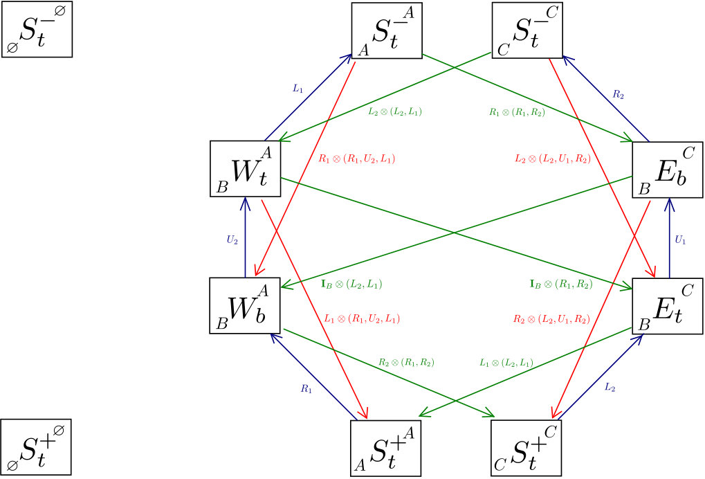 Figure 1
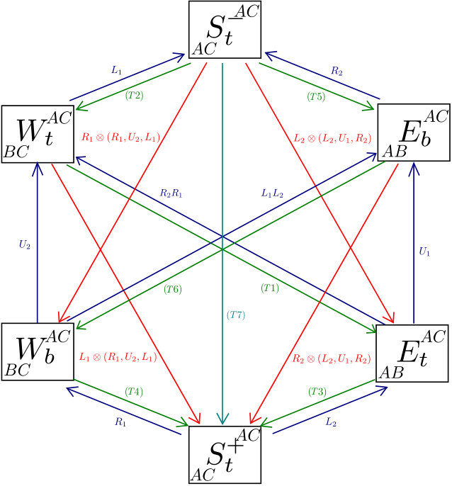 Figure 2
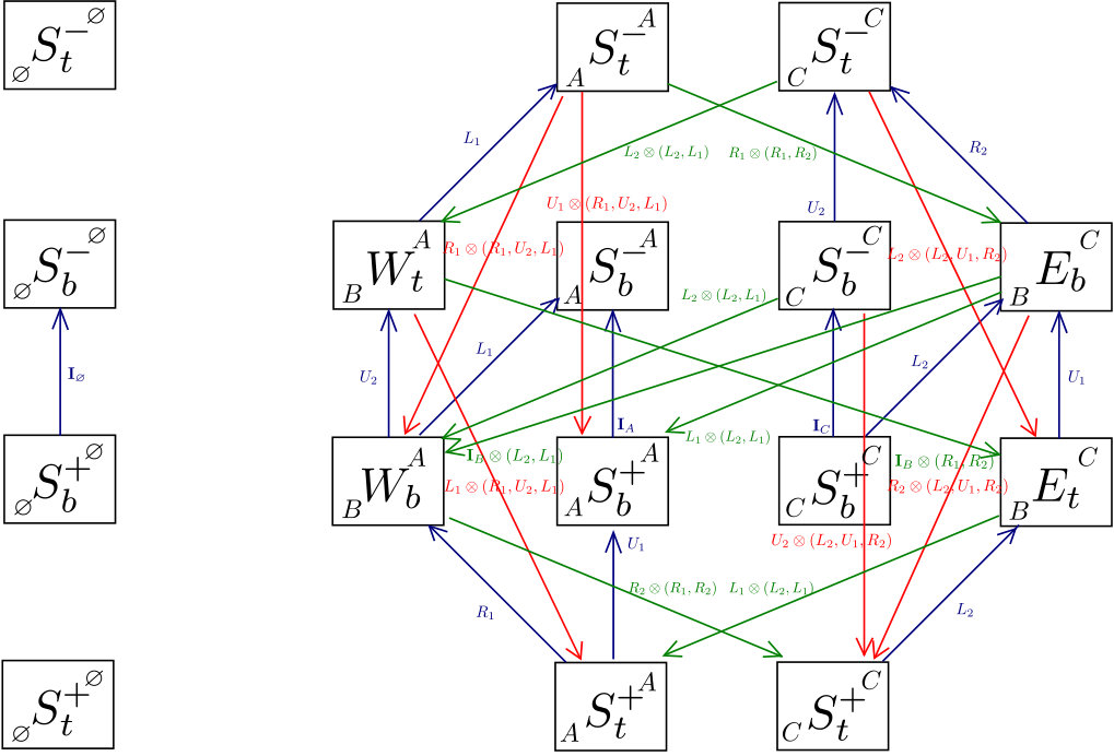 Figure 3
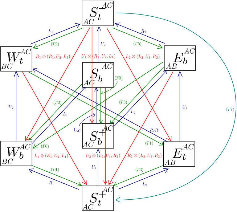 Figure 4
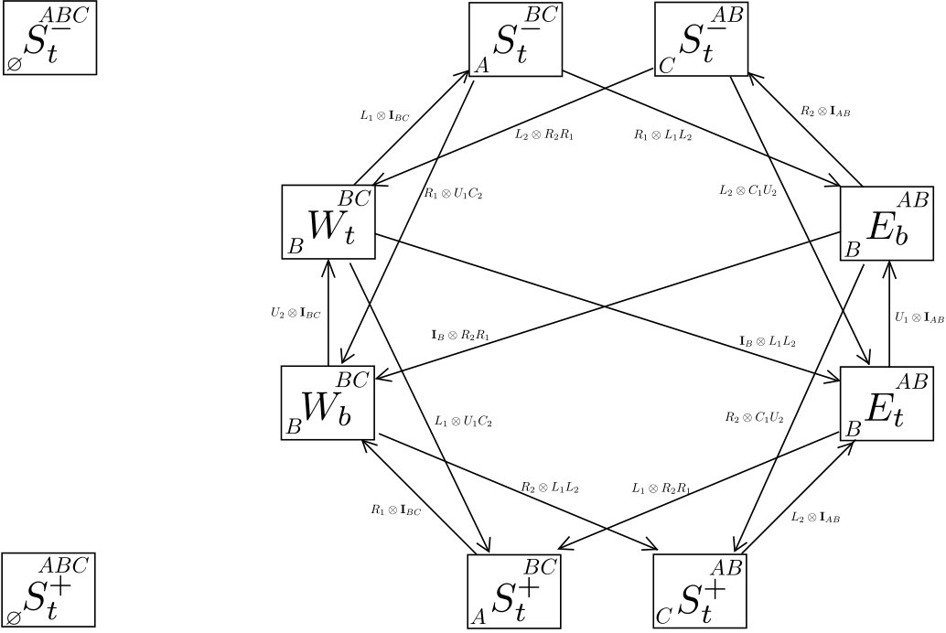 Figure 5
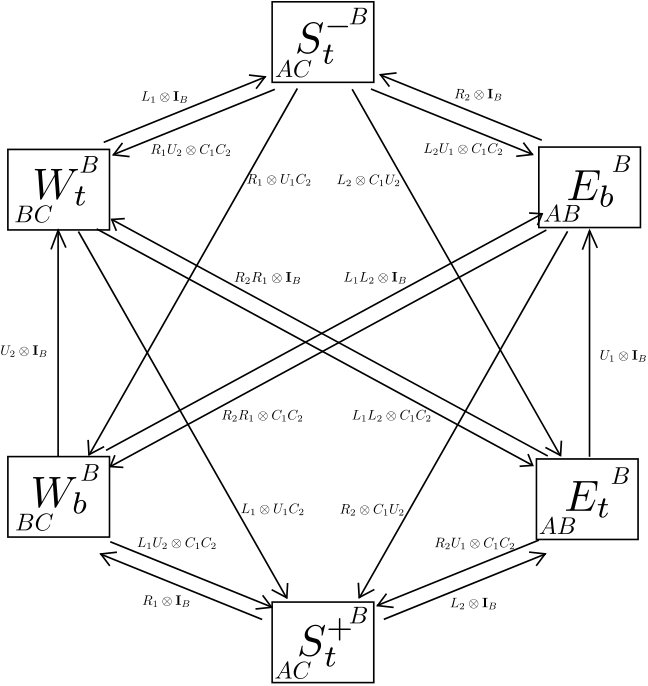 Figure 6
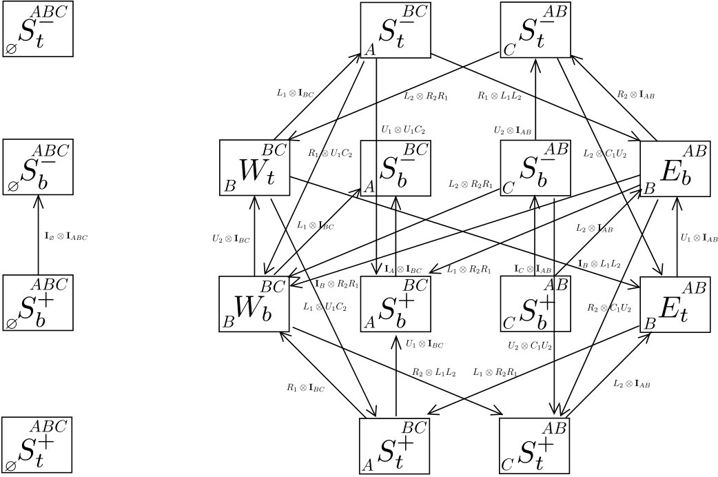 Figure 7
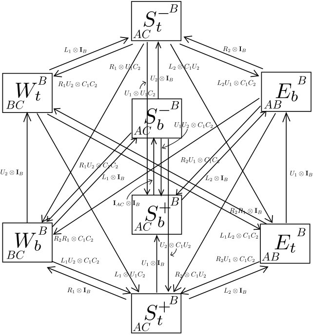 Figure 8
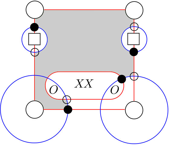 Figure 9
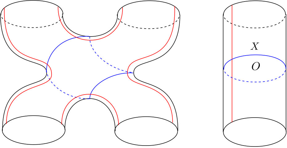 Figure 10
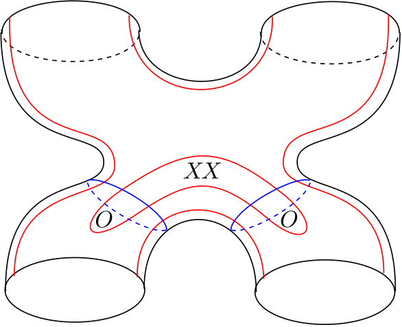 Figure 11
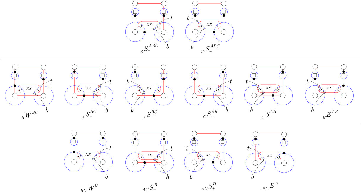 Figure 12
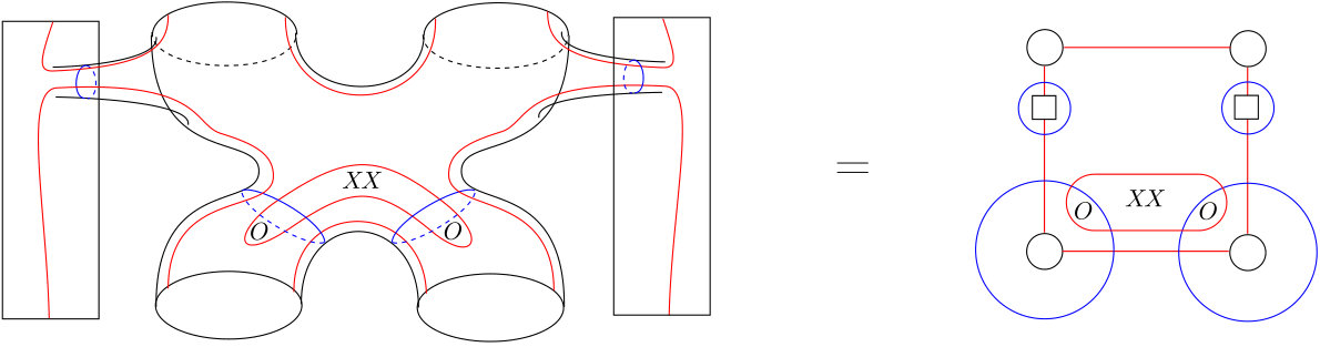 Figure 13