Quasinormal modes of regular black holes with non linear-Electrodynamical sources
Grigoris Panotopoulos, \'Angel Rinc\'on

TL;DR
This paper calculates the quasinormal mode spectrum of regular black holes influenced by Non-Linear Electrodynamics, analyzing stability and effects of charge, angular momentum, and overtone number using WKB approximation.
Contribution
It provides the first detailed analysis of quasinormal modes for regular black holes with Non-Linear Electrodynamics, including an analytical eikonal limit expression.
Findings
All modes are stable.
Charge, angular momentum, and overtone number significantly affect the spectrum.
Comparison with other charged black holes highlights unique spectral features.
Abstract
We compute the spectrum of quasinormal frequencies of regular black holes obtained in the presence of Non-Linear Electrodynamics. In particular, we perturb the black hole with a minimally coupled massive scalar field, and we study the corresponding perturbations adopting the 6th order WKB approximation. We analyze in detail the impact on the spectrum of the charge of the black hole, the quantum number of angular momentum and the overtone number. All modes are found to be stable. Finally, a comparison with other charged black holes is made, and an analytical expression for the quasinormal spectrum in the eikonal limit is provided.
Click any figure to enlarge with its caption.
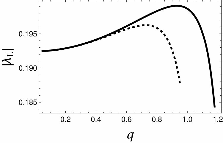 Figure 1
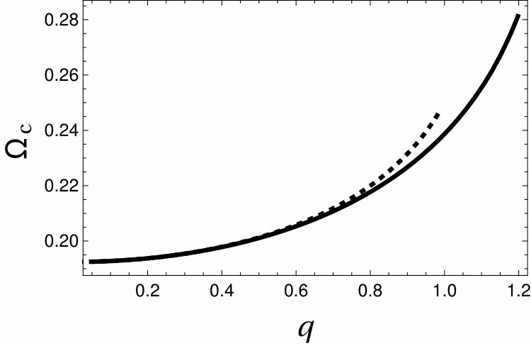 Figure 2
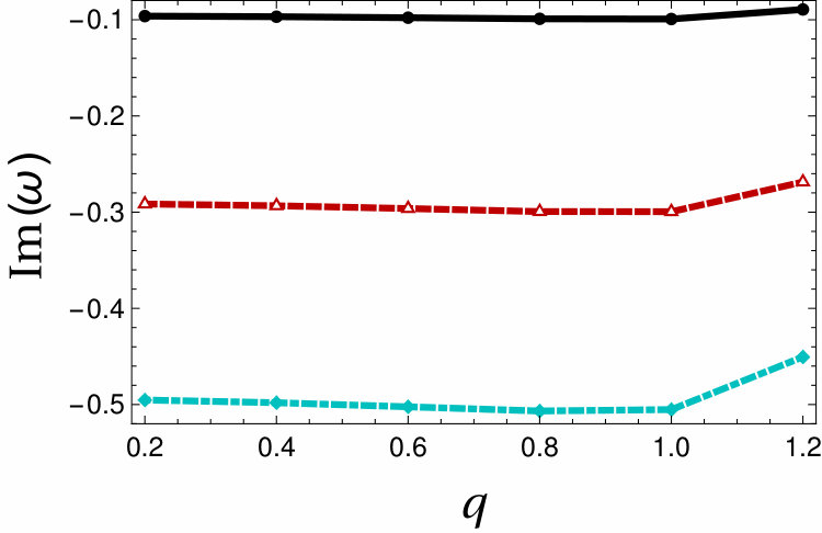 Figure 3
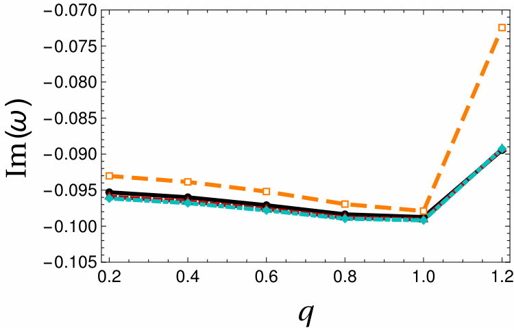 Figure 4
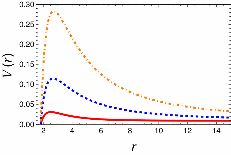 Figure 5
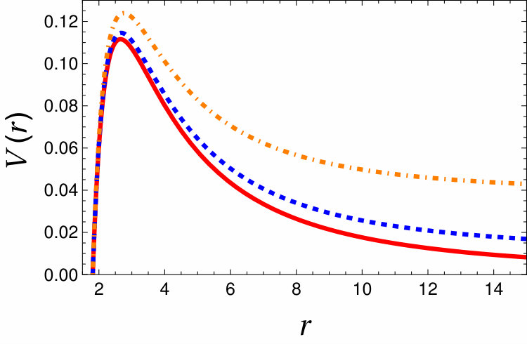 Figure 6
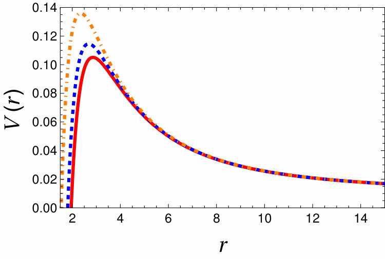 Figure 7
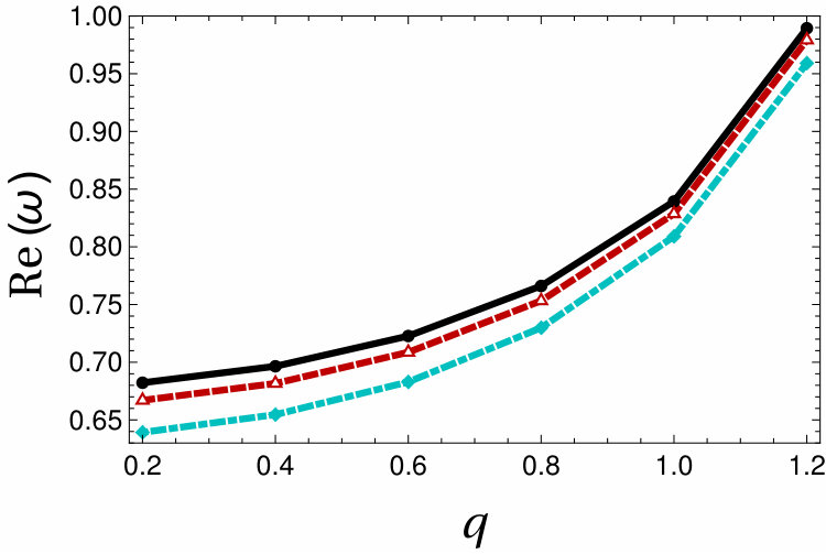 Figure 8
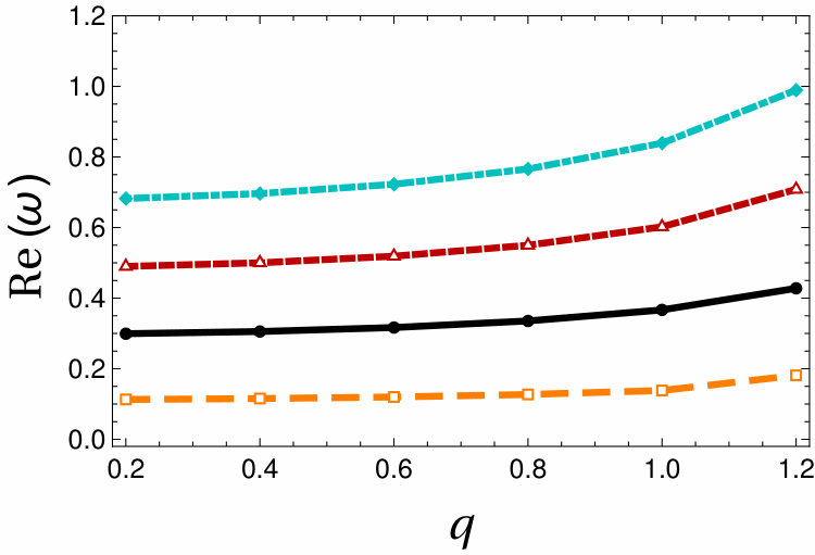 Figure 9
| 0 | 0.1130-0.0930 i | 0.2993-0.0953 i | 0.4900-0.0959 i | 0.6823-0.0961 i |
| (0.1113-0.1010 i) | (0.2949-0.0980 i) | (0.4869-0.0970 i) | (0.6799-0.0967 i) | |
| 1 | 0.4689-0.2939 i | 0.6670-0.2915 i | ||
| (0.4673-0.2962 i) | (0.6653-0.2929 i) | |||
| 2 | 0.6393-0.4952 i | |||
| (0.6385-0.4970 i) |
| 0 | 0.1155-0.0939 i | 0.3055-0.0960 i | 0.5002-0.0966 i | 0.6965-0.0968 i |
| (0.1137-0.1016 i) | (0.3012-0.0985 i) | (0.4972-0.0976 i) | (0.6943-0.0973 i) | |
| 1 | 0.4796-0.2957 i | 0.6817-0.2933 i | ||
| (0.4781-0.2979 i) | (0.6800-0.2947 i) | |||
| 2 | 0.6547-0.4981 i | |||
| (0.6539-0.4997 i) |
| 0 | 0.1200-0.0952 i | 0.3168-0.0971 i | 0.5190-0.0976 i | 0.7227-0.0978 i |
| (0.1181-0.1025 i) | (0.3127-0.0994 i) | (0.5161-0.0986 i) | (0.7206-0.0983 i) | |
| 1 | 0.4994-0.2985 i | 0.7087-0.2962 i | ||
| (0.4979-0.3005 i) | (0.7071-0.2975 i) | |||
| 2 | 0.6830-0.5023 i | |||
| (0.6822-0.5038 i) |
| 0 | 0.1272-0.0969 i | 0.3354-0.0984 i | 0.5499-0.0988 i | 0.7661-0.0990 i |
| (0.1252-0.1036 i) | (0.3317-0.1004 i) | (0.5473-0.0996 i) | (0.7642-0.0994 i) | |
| 1 | 0.5322-0.3014 i | 0.7533-0.2994 i | ||
| (0.5307-0.3032 i) | (0.7518-0.3005 i) | |||
| 2 | 0.7299-0.5067 i | |||
| (0.7291-0.5080 i) |
| 0 | 0.1384-0.0979 i | 0.3667-0.0987 i | 0.6022-0.0991 i | 0.8394-0.0992 i |
| (0.1364-0.1036 i) | (0.3635-0.1003 i) | (0.6000-0.0997 i) | (0.8377-0.0995 i) | |
| 1 | 0.5874-0.3011 i | 0.8287-0.2995 i | ||
| (0.5861-0.3026 i) | (0.8274-0.3004 i) | |||
| 2 | 0.8091-0.5052 i | |||
| (0.8083-0.5063 i) |
| 0 | 0.1812-0.0724 i | 0.4280-0.0894 i | 0.7083-0.0893 i | 0.9894-0.0893 i |
| (0.1525-0.0885 i) | (0.4261-0.0902 i) | (0.7068-0.0896 i) | (0.9883-0.0894 i) | |
| 1 | 0.6938-0.2697 i | 0.9793-0.2686 i | ||
| (0.6928-0.2704 i) | (0.9783-0.2690 i) | |||
| 2 | 0.9593-0.4504 i | |||
| (0.9583-0.4512 i) |
| RN | Regular BH | |
|---|---|---|
| 0.20 | 0.299354-0.095294 i | 0.299347-0.095295 i |
| 0.40 | 0.305624-0.095966 i | 0.305500-0.095993 i |
| 0.60 | 0.317575-0.096893 i | 0.316803-0.097092 i |
| 0.80 | 0.338881-0.097145 i | 0.335447-0.098359 i |
| 0.95 | 0.367320-0.093187 i | 0.357181-0.098879 i |
| 0.99 | 0.378067-0.089483 i | 0.364714-0.098785 i |
| RN | Regular BH | |
|---|---|---|
| 0.20 | 0.490056-0.095905 i | 0.490044-0.095907 i |
| 0.40 | 0.500432-0.096541 i | 0.500231-0.096570 i |
| 0.60 | 0.520216-0.097403 i | 0.518963-0.097612 i |
| 0.80 | 0.555564-0.097572 i | 0.549923-0.098800 i |
| 0.95 | 0.603642-0.093650 i | 0.586164-0.099245 i |
| 0.99 | 0.622997-0.089806 i | 0.598769-0.099130 i |
Peer Reviews
No public reviews on file for this paper yet. If you reviewed it on a platform where reviews are public (OpenReview, ICLR, NeurIPS, ICML), you can paste yours below so the community can read it here.
Videos
No videos yet. Explain this paper in a talk, walkthrough, or lecture? Add one.
11institutetext: Centro de Astrofísica e Gravitação, Departamento de Física, Instituto Superior Técnico-IST,
Universidade de Lisboa-UL, Av. Rovisco Pais, 1049-001 Lisboa, Portugal 22institutetext: Instituto de Física, Pontificia Universidad Católica de Valparaíso, Avenida Brasil 2950, Casilla 4059, Valparaíso, Chile
Quasinormal modes of regular black holes with Non-Linear-Electrodynamical sources
Grigoris Panotopoulos E-mail: [email protected]11
Ángel Rincón E-mail: [email protected]22
(Received: date / Revised version: date)
Abstract
We compute the spectrum of quasinormal frequencies of regular black holes obtained in the presence of Non-Linear Electrodynamics. In particular, we perturb the black hole with a minimally coupled massive scalar field, and we study the corresponding perturbations adopting the 6th order WKB approximation. We analyze in detail the impact on the spectrum of the charge of the black hole, the quantum number of angular momentum and the overtone number. All modes are found to be stable. Finally, a comparison with other charged black holes is made, and an analytical expression for the quasinormal spectrum in the eikonal limit is provided.
1 Introduction
Although black holes (BHs) and gravitational waves (GWs) are predicted to exist within the framework of Einstein’s General Relativity (GR) GR , until a few years ago there was only indirect evidence for the existence of both of them. Galactic centres are supposed to host supermassive BHs SMBH1 ; SMBH2 ; SMBH3 , while gravitational waves had been indirectly seen in orbital decay of binary systems due to emission of gravitational radiation Binary . The historical LIGO direct detection of GWs ligo1 ; ligo2 ; ligo3 has provided the strongest evidence so far that BHs do exist in Nature and that they merge, and it has opened a completely new window to the Universe. Despite the fact that BHs are the simplest objects in the Universe, characterized entirely by a handful of parameters, such as mass, spin and charges, they are fascinating objects bringing together many different areas, from gravitation to thermodynamics to quantum mechanics, and they are of paramount importance to gravitation, since they have the potential of revealing (at least) some of the hidden secrets of quantum gravity.
A special attention is devoted to non-linear electrodynamics (NLE), which has a long history and it has been studied over the years in several different contexts. Maxwell’s classical theory is based on a system of linear equations, but when quantum effects are taken into account, the effective equations become non-linear. The first models go back to the 30’s when Euler and Heisenberg obtained QED corrections Euler , while Born and Infeld obtained a finite self-energy of point-like charges BI . Furthermore, a non-trivial extension of Maxwell’s theory leads to the by now well-known Einstein-power-Maxwell (EpM) theory described by a Lagrangian density of the form , where is the usual Maxwell invariant, to be defined below, and is an arbitrary rational number. This class of theories maintain the nice properties of conformal invariance in any number of space time dimensionality provided that . Black hole solutions in (1+2)-dimensional and higher-dimensional EpM theories have been obtained in BH1 and BH2 respectively (see also SD1 ; SD2 for scale-dependent black holes in the presence of EpM NLE). More exotic NLE models, such as logarithmic Soleng:1995kn , rational Kruglov_2014 , and exponential Hendi:2013dwa among others, have been studied in connection to black hole physics.
Furthermore, the well-known Reissner-Nordström black hole solution RN is a charged solution to Einstein’s field equations coupled to Maxwell’s linear electrodynamics, and it is characterized by a singularity at the center. The singularity is hidden by an event horizon, and therefore it has no effect on the outside region, where Physics is well-behaved. The existence of singularities, however, indicate the breakdown of General Relativity, and so attempts are made to obtain regular BH solutions, such as the solution obtained for the first time by Bardeen Bardeen1 , see also borde ; Bardeen2 . In borde this class of black holes was named “Bardeen black holes”, while in Bardeen2 it was shown that the Bardeen model could be obtained within Einstein’s General Relativity coupled to an appropriate non-linear electromagnetic source. Nowadays several regular black hole solutions are known, which have been obtained applying the same approach, that is assuming appropriate non-linear electromagnetic sources, which in the weak field limit are reduced to the standard Maxwell’s linear theory. It is an approach that allows us to generate a new class of solutions to Einstein’s field equations beato1 ; beato2 ; beato3 ; bronnikov ; dymnikova ; hayward ; vagenas1 ; vagenas2 ; culetu , which on the one hand have a horizon, and on the other hand their curvature invariants, such as the Ricci scalar , are regular everywhere, as opposed to the standard Reissner-Nordström solution. Regular BHs may help us understand the final states of gravitational collapse ellis ; extra , which is not possible when singularities are present.
Quasinormal modes (QNMs) are complex numbers that encode the information on how the black holes relax after the perturbation is applied. They depend on the type of perturbation (scalar, vector etc) and on the properties of the geometry itself, and they do no depend on initial conditions. The work of wheeler marked the birth of BH perturbations, and it was later extended by zerilli1 ; zerilli2 ; zerilli3 ; moncrief ; teukolsky . A comprehensive overview of BH perturbations is summarized in Chandrasekhar’s monograph monograph . Black hole perturbation theory and QNMs are relevant during the ringdown phase, in which a distorted object after the merging of two black holes is formed, and the geometry of spacetime undergoes dumped oscillations due to the emission of gravitational waves. For a review on the subject see review1 , and for a more recent ones review2 ; review3 .
Given the interest in gravitational wave Astronomy and on QNMs of black holes, it would be interesting to see what kind of QN spectra are expected from regular BHs. In previous works quasinormal modes of regular black holes were computed by several authors, see e.g. correa ; lemos ; otro ; wu ; ahmedov1 ; ahmedov2 ; bambi ; ahmedov3 . It is the goal of the present article to compute the QNMs of regular charged black holes in the presence of non-linear electrodynamics assuming a massive scalar field as the test particle that perturbs the black hole. In particular, we shall consider one of the black holes obtained in vagenas2 employing mass distribution functions. This regular black hole has already been discussed in wu , our work however is different in several respects. In particular, i) we study scalar instead of gravitational perturbations, ii) we compute the QNMs for more values of the charge of the black hole approaching extremality, and iii) we adopt the WKB method of sixth order instead of third.
The plan of our work is the following: After this Introduction, we present the theory and the regular BH solution in subsection 2.1, and the wave equation for scalar perturbations in subsection 2.2. In the third Section we compute the QNMs of the black holes in the WKB approximation and we discuss our results. Finally, we conclude our work in Section 4. We use natural units such that and metric signature .
2 Formalism
2.1 Regular black hole in the presence of NLE
Let us consider a 4-dimensional theory described by the action
[TABLE]
where is the Ricci scalar, the determinant of the metric tensor , , and the Maxwell invariant with being the electromagnetic field strength.
Varying the action with respect to the Maxwell potential one obtains the generalized Maxwell equations vagenas2
[TABLE]
where we define . Furthermore, varying the action with respect to the metric tensor one obtains Einstein’s field equations
[TABLE]
where is the Einstein tensor, while the matter stress-energy tensor corresponds to the electromagnetic energy-momentum tensor vagenas2
[TABLE]
We seek spherically symmetric static solutions of the form
[TABLE]
but instead of specifying the Lagrangian density to obtain the metric function , we assume that the solution for the metric lapse function corresponds to a known function instead vagenas2
[TABLE]
where are the mass and the electric charge of the black hole, respectively. Among several possible choices we have opted for this particular regular black hole since the exponential function is a common place in Physics. A couple of notable examples are for instance the Liouville-type potential for the dilaton expo1 or the Yukawa potential in nuclear physics that inspired the study of Yukawa black holes expo2 .
Introducing the distribution function , the temporal and radial components of Einstein’s equations read
[TABLE]
while the angular components read
[TABLE]
Finally, the generalized Maxwell’s equations are equivalent to the following equation
[TABLE]
where the prime denotes differentiation with respect to , and is the electric field. Combining the equations of motion one can determine the electric field as well as the electromagnetic Lagrangian density as functions of the radial coordinate
[TABLE]
and so one obtains the electromagnetic Lagrangian in parametric form , . Finally, the Ricci scalar is computed to be
[TABLE]
and it is regular everywhere.
2.2 Perturbations for a test massive scalar field
First we consider a four-dimensional spherically symmetric fixed gravitational background of the form
[TABLE]
where the metric function is given by vagenas2
[TABLE]
with and being the mass and the electric charge of the black hole, respectively. Clearly, when we recover the Schwarzschild solution for a neutral BH, while expanding in powers of we obtain the following approximate expression
[TABLE]
The first 3 terms are precisely the ones corresponding to the well–known RN black hole solution, while higher powers are corrections to that.
Then, we perturb the black hole with a probe minimally coupled massive scalar field with equation of motion
[TABLE]
where is the mass of the test scalar field. We separate variables making the standard ansatz
[TABLE]
with being the spherical harmonics, and we obtain a Schrödinger-like equation of the form
[TABLE]
with being the so–called tortoise coordinate
[TABLE]
while the effective potential is given by the expression
[TABLE]
where the prime denotes differentiation with respect to . The effective potential as a function of the radial coordinate can be seen in Figure (1). The left panel shows the impact of angular momentum, the right panel shows the impact of the mass of the test scalar field that perturbs the black hole, while the panel in the middle shows the impact of the electric charge of the black hole.
To complete the formulation of the physical problem at hand we must add the appropriate boundary conditions, both at infinity and at the horizon, to the Schrödinger-like equation. For asymptotically flat spacetimes we impose the quasinormal condition valeria .
[TABLE]
where the parameters are arbitrary constants. The physical meaning of the required boundary conditions is the following: i) on the one hand the purely ingoing wave expresses the fact that nothing escapes from the horizon, and ii) on the other hand the purely outgoing wave corresponds to the requirement that no radiation comes from infinity valeria . It is precisely the quasinormal condition that allows us to obtain an infinite set of discrete complex numbers, which are the so-called quasinormal frequencies of the black hole.
Given the time dependence of the scalar field, , the mode grows exponentially (in other words it is unstable) when , or decays exponentially (it is stable) when . In the latter case the real part determines the frequency of the oscillation, , while the inverse of determines the dumping time, .
3 QNMs of regular BHs in the WKB approximation
3.1 Numerical results
An exact computation of the QNMs of black holes in an analytical way is possible only in some cases, see e.g. potential ; ferrari ; cardoso2 ; exact1 ; exact2 ; exact3 ; exact4 ; exact5 ; exact6 ; Ovgun:2018gwt ; Rincon:2018ktz . Semi-analytical approaches based on the popular WKB approximation wkb1 ; wkb2 (for an improved semi-analytical approach see improved ) have been extensively applied to several cases. For previous similar works see e.g. paper1 ; paper2 ; paper3 ; paper4 ; paper5 ; paper6 , and for more recent works see e.g. correa ; paper8 ; paper9 ; paper10 ; Rincon:2018sgd , and references therein.
The QN frequencies may be computed using the formula
[TABLE]
where is the maximum of the effective potential, is its second derivative evaluated at the maximum, is the so-called overtone number, , while are non-trivial expressions of and higher derivatives of the potential evaluated at the maximum, and can be seen e.g. in correa ; paper2 .
In the present work we have made use of the Wolfram Mathematica wolfram code with WKB at any order from one to six (here we have worked in 6th order) presented in code . We have fixed the mass of the black hole to be , the mass of the test scalar field is taken to be either or , while for the electric charge we have considered 6 values from 0.2 to 1.2 (the extremal black hole is obtained for ), so that the numerical results go smoothly to the Schwarzschild limit as . In cardoso3 it was shown that the WKB approximation works very well for , and therefore here we shall consider the cases i) , ii) and iii) . We have also included the lowest multiple since it corresponds to the fundamental mode, although we do not expect the approximation to be very good. Finally, we consider non-extremal black holes (for the extremal case see extremal ), while the eikonal regime will be considered separately in the end before concluding our work.
Our numerical results for the QN modes of the charged regular black holes are summarized in the tables below. In the last 2 tables we have made a direct comparison between regular black holes and the standard Reissner-Nordström (RN) black hole RN for and . The values of the frequencies corresponding to the massless scalar field case are shown in parenthesis. We see that for the real part is lower, while the imaginary part is more negative compared to the case.
For better visualization we show graphically how the QNMs depend on the angular momentum, the overtone number as well as the electromagnetic coupling. In particular, the first row of 3 shows the real and imaginary part of the frequencies versus for 3 different values of the overtone number and fixed angular momentum , while the second row of the same figure shows the real and imaginary part of the frequencies versus for 4 different values of angular momentum and fixed . The real part increases with the electric charge and with the angular momentum, like in the case of RN. In other theories too, such as Born-Infeld and Gauss-Bonnet gravity, the real part of QNM of charged BH increases with the electric charge paper4 ; paper5 . The imaginary part becomes more and more negative with the electric charge, and less and less negative with the angular momentum, like in the RN case RN2 . Notice that the characteristic minimum of the imaginary part (or maximum if one plots versus ) for a certain value of the electric charge close to its extremal value is observed, like in the RN case (also observed in paper10 for charged BHs in the EpM theory) and contrary to Born-Infeld NLE and Gauss-Bonnet gravity, where the imaginary part is a monotonic function of the electric charge paper4 ; paper5 .
3.2 QNMs in the eikonal limit
In the eikonal regime () the WKB approximation becomes increasingly accurate, and therefore one can obtain analytical expressions for the QN frequencies. In the eikonal limit () it is the angular momentum term that dominates in the expression for the effective potential
[TABLE]
where for convenience we have introduced a new function . It is not difficult to verify that the maximum of the potential is located at the point , which may be computed solving the following algebraic equation
[TABLE]
Then, following the formalism developed in eikonal1 , the QNMs in the eikonal regime are computed by
[TABLE]
where the Lyapunov exponent is given by eikonal1
[TABLE]
while the angular velocity at the unstable null geodesic is given by eikonal1
[TABLE]
Notice that the same expressions for and for may be obtained applying the WKB approximation of 1st order, as it was done e.g. in Ponglertsakul:2018smo . Therefore, although in the presence of non-linear electromagnetic sources photons follow the null trajectories of an effective geometry rather than the null geodesics of the true geometry eikonal2 ; eikonal3 ; ref2 , the previous expressions for and for remain the same. We see that the angular velocity determines the real part of the modes, where only the degree of angular momentum enters, while the Lyapunov exponent determines the imaginary part of the modes, where only the overtone number enters. In Fig. (2) we show the angular velocity (left panel) as well as the Lyapunov exponent (right panel) as a function of for . For comparison reasons we show in the same figure the corresponding quantities for the standard RN solution. The angular velocity increases monotonically with the electric charge, while the Lyapunov exponent reaches a maximum value first and then it decreases as opposed to the Bardeen black hole studied in correa , where it was found that decreases monotonically with . The angular velocity of the regular BH lies below of the RN BH, while the Lyapunov exponent of the regular BH lies above of the RN solution. The figure show that for the same BH parameters and the same angular degree , the regular BH solution is characterized by a lower real part and a higher imaginary part, and the differences grow as we approach extremality.
Finally, when studying the QNMs of a black hole stability of the system is one of the most important results. The conditions obtained in Moreno allow us to make a simple test on the dynamical stability of the black hole studied here. The conditions are the following
[TABLE]
where is the Hamiltonian density of the system, and . These conditions should hold for any or in the range , where . For the exponential mass distribution function considered in this work the Hamiltonian is computed to be vagenas2
[TABLE]
where , , and is given by
[TABLE]
The Hamiltonian density as a function of is found to be
[TABLE]
and its derivatives can be computed in a straightforward manner. It is easy to verify that all the aforementioned conditions are satisfied for and .
4 Conclusions
In this article we have computed the quasinormal modes of four-dimensional charged regular black holes in the presence of Non-Linear Electrodynamical sources. We have studied scalar perturbations using a Schrödinger-like equation with the appropriate effective potential, and we have adopted the popular and extensively used WKB approximation of 6th order. Our numerical results are summarized in tables, and we have shown graphically the impact on the spectrum of the electric charge of the black hole as well as of the overtone number and of the quantum number of angular momentum. All modes are found to be stable. A comparison with the RN and other charged black holes is made, and an analytical expression for the QN spectrum in the eikonal limit has been obtained.
Acknowlegements
We wish to thank the anonymous reviewer for useful comments and suggestions. The author G. P. thanks the Fundação para a Ciência e Tecnologia (FCT), Portugal, for the financial support to the Center for Astrophysics and Gravitation-CENTRA, Instituto Superior Técnico, Universidade de Lisboa, through the Grant No. UID/FIS/00099/2013. The author A. R. acknowledges DI-VRIEA for financial support through Proyecto Postdoctorado 2019 VRIEA-PUCV.
The reference list from the paper itself. Each links out to its DOI / PubMed record.
- 1(1) A. Einstein, Annalen Phys. 49 (1916) 769–822.
- 2(2) S. M. Liu, V. Petrosian and F. Melia, Astrophys. J. 611 (2004) L 101 [astro-ph/0403487].
- 3(3) G. Trap et al. , Adv. Space Res. 45 (2010) 507 [ar Xiv:0910.0399 [astro-ph.HE]].
- 4(4) A. Hees et al. , Phys. Rev. Lett. 118 (2017) no.21, 211101 [ar Xiv:1705.07902 [astro-ph.GA]].
- 5(5) J. M. Weisberg, D. J. Nice and J. H. Taylor, Astrophys. J. 722 (2010) 1030 [ar Xiv:1011.0718 [astro-ph.GA]].
- 6(6) B. P. Abbott et al. [LIGO Scientific and Virgo Collaborations], Phys. Rev. Lett. 116 (2016) no.6, 061102 [ar Xiv:1602.03837 [gr-qc]].
- 7(7) B. P. Abbott et al. [LIGO Scientific and Virgo Collaborations], Phys. Rev. Lett. 116 (2016) no.24, 241103 [ar Xiv:1606.04855 [gr-qc]].
- 8(8) B. P. Abbott et al. [LIGO Scientific and VIRGO Collaborations], Phys. Rev. Lett. 118 (2017) no.22, 221101 [ar Xiv:1706.01812 [gr-qc]].