Performance-oriented model learning for data-driven MPC design
Dario Piga, Marco Forgione, Simone Formentin, Alberto Bemporad

TL;DR
This paper introduces a novel data-driven approach to optimize model learning for MPC, focusing on enhancing closed-loop performance by selecting the best prediction model through Bayesian optimization.
Contribution
It applies the 'identification for control' concept to hierarchical MPC using Bayesian optimization, a first in this context, to improve control performance.
Findings
Enhanced closed-loop performance with data-driven model selection
Successful application of Bayesian optimization in hierarchical MPC
Improved robustness without conservative assumptions
Abstract
Model Predictive Control (MPC) is an enabling technology in applications requiring controlling physical processes in an optimized way under constraints on inputs and outputs. However, in MPC closed-loop performance is pushed to the limits only if the plant under control is accurately modeled; otherwise, robust architectures need to be employed, at the price of reduced performance due to worst-case conservative assumptions. In this paper, instead of adapting the controller to handle uncertainty, we adapt the learning procedure so that the prediction model is selected to provide the best closed-loop performance. More specifically, we apply for the first time the above "identification for control" rationale to hierarchical MPC using data-driven methods and Bayesian optimization.
Click any figure to enlarge with its caption.
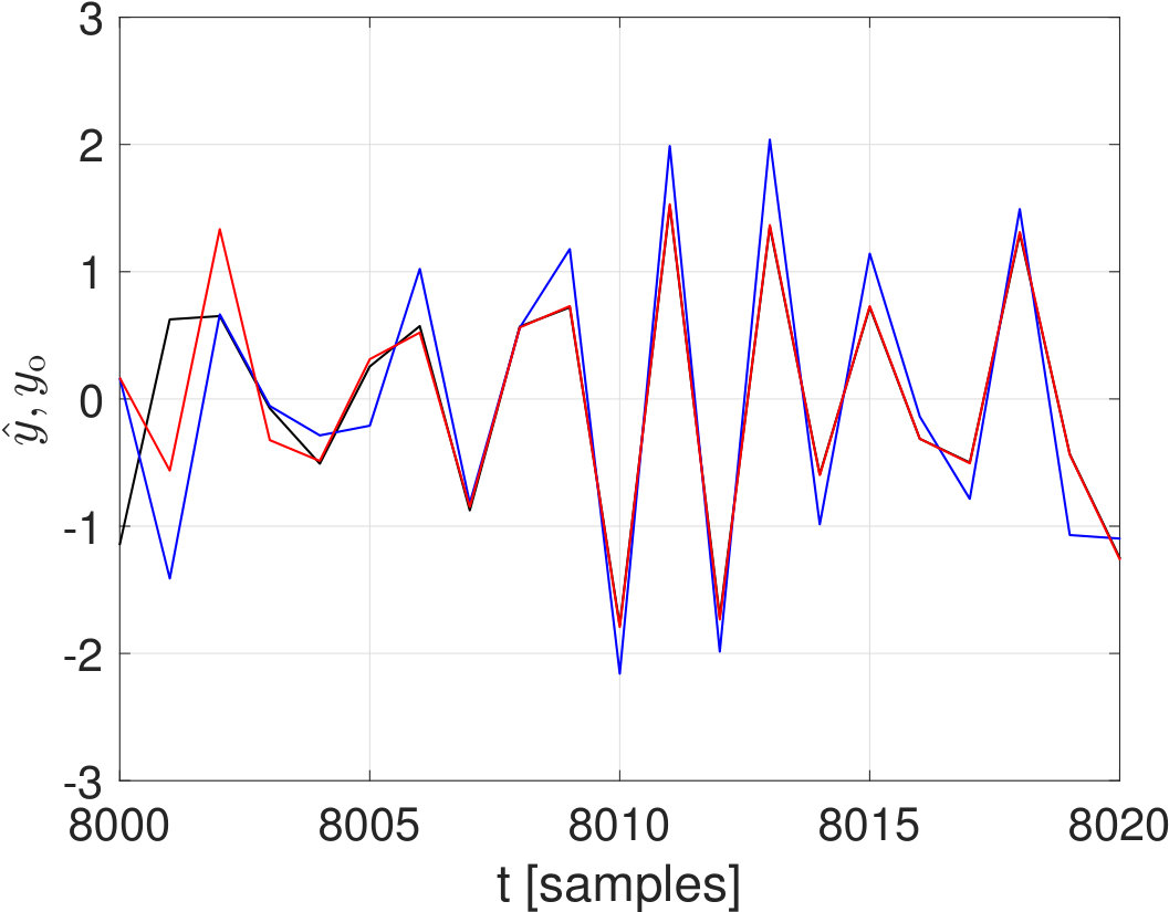 Figure 1
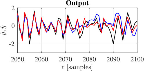 Figure 2
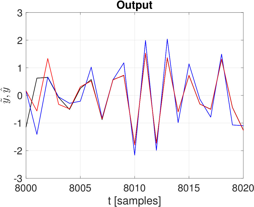 Figure 3
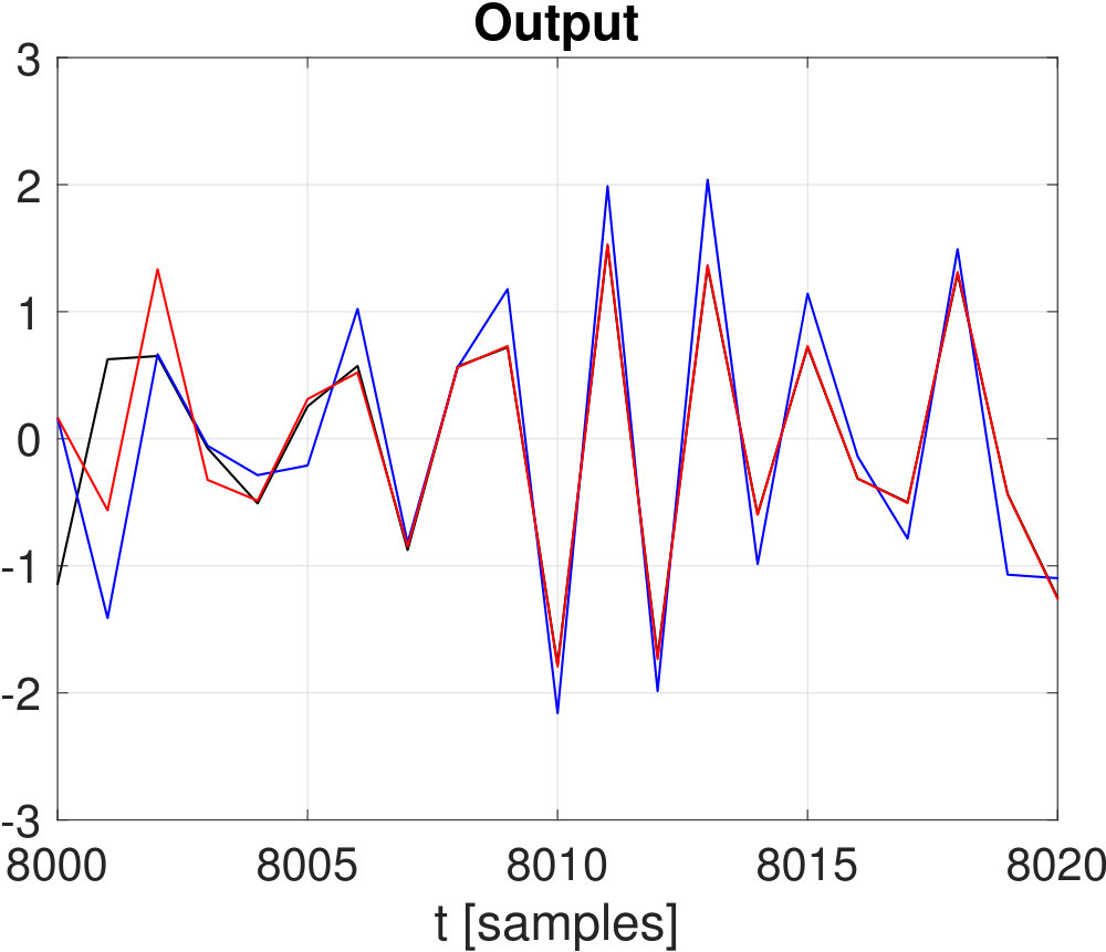 Figure 4
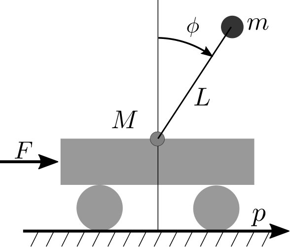 Figure 5
 Figure 6
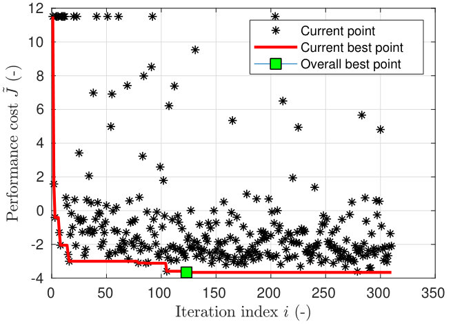 Figure 7
 Figure 8
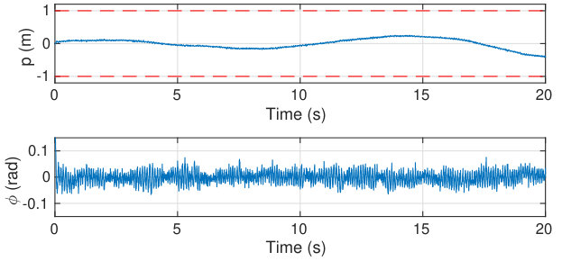 Figure 9
Peer Reviews
No public reviews on file for this paper yet. If you reviewed it on a platform where reviews are public (OpenReview, ICLR, NeurIPS, ICML), you can paste yours below so the community can read it here.
Videos
No videos yet. Explain this paper in a talk, walkthrough, or lecture? Add one.
Performance-oriented model learning for data-driven MPC design
Dario Piga, Marco Forgione, Simone Formentin, Alberto Bemporad This work was partially supported by the H2020-723248 project DAEDALUS - Distributed control and simulation platform to support an ecosystem of digital automation developers and by the Lombardia region and the Cariplo foundation, under the project Learning to Control (L2C), no. 2017-1520.D. Piga and M. Forgione are with IDSIA Dalle Molle Institute for Artificial Intelligence SUPSI-USI, Manno, Switzerland. [email protected]; [email protected]. Formentin is with the Dipartimento di Elettronica e Informazione, Politecnico di Milano, Milano, Italy. [email protected]. Bemporad is with IMT School for Advanced Studies Lucca, Lucca, Italy [email protected]
Abstract
Model Predictive Control (MPC) is an enabling technology in applications requiring controlling physical processes in an optimized way under constraints on inputs and outputs. However, in MPC closed-loop performance is pushed to the limits only if the plant under control is accurately modeled; otherwise, robust architectures need to be employed, at the price of reduced performance due to worst-case conservative assumptions. In this paper, instead of adapting the controller to handle uncertainty, we adapt the learning procedure so that the prediction model is selected to provide the best closed-loop performance. More specifically, we apply for the first time the above “identification for control” rationale to hierarchical MPC using data-driven methods and Bayesian optimization.
Index Terms:
Predictive control for nonlinear systems, Identification for control, Machine learning.
I Introduction
Nowadays, Model Predictive Control (MPC) has become the most popular advanced control technology for several complex engineering applications [1]. Apart from computational aspects, it is widely recognized that one key practical challenge in MPC arises when dealing with uncertainty, especially when the prediction model is identified using open-loop data taken from a specific operation of the plant [2].
In case of partially known systems, traditional MPC approaches exhibit some degree of robustness, so that marginal robust performance can be guaranteed. When intrinsic robustness of deterministic MPC is not enough, robust MPC [3] and stochastic MPC [2] approaches have been developed to take into account uncertainties. However, regardless of the specific technique, increasing robustness of the MPC controller usually leads to conservative performance [4].
While there is usually a separation between model identification and control design, an alternative approach to managing uncertainty in designing control systems is to revisit the identification process as a procedure to be designed by bearing the final control application in mind. Such a rationale is known as Identification for Control (I4C) and has been widely studied for fixed-order (oftentimes, PID) control of Linear Time-Invariant (LTI) systems [5]. According to I4C, the best model for control may not be the one providing the least output prediction errors, but the one providing the best performance on the true system when in closed loop with the associated model-based controller.
As far as we are aware of, the I4C modeling approach has never been applied to MPC control. Learning techniques have instead been shown to be useful for iterative MPC tasks in [6] and in reinforcement learning applied to MPC [7]. Furthermore, data-driven approaches have been proposed for direct MPC optimization using open- and closed-loop data, see, e.g., [8, 9]. Although the above approaches are powerful tools for control design in case of unknown systems, they fail to provide a mathematical (albeit control-oriented) description of the plant. Indeed, the latter can often be useful for physical interpretation, performance monitoring, and diagnosis [10].
In this work, we propose an Identification for (Model-Predictive) Control approach aimed at finding the best prediction model for MPC from experimental data, by considering the control objective directly in the model learning phase. We propose a hierarchical architecture, typically employed in several industrial applications, in which the inner controller is a parametric filter (e.g., a PID controller) aimed to stabilize the system at a fast pace, whereas the outer loop plays the role of a reference governor (RG) [11, 12] with a twofold goal: () boosting the performance of the inner loop and () handling the signals constraints due, e.g., to actuator bounds or system limitations. Within this framework, the RG is typically an MPC law based on a model of the inner loop. According to the I4C philosophy, we propose a change of perspective and treat such a model as a design parameter instead. Such a parameter will be iteratively optimized, together with the inner controller, using closed-loop data collected on the plant and Bayesian optimization. Finally, we show that, using the same rationale and tools, also the prediction horizon, a critical parameter to tune in MPC, can be optimized from data.
For the sake of completeness, the first use of Bayesian optimization in control-oriented identification was proposed in [13], based on a simpler control scheme. The same hierarchical architecture was instead addressed in [9] to design the controller from data, but without providing an MPC-oriented model of the plant.
The remainder of the paper is as follows. In Section II the control problem of interest is formally stated. The hierarchical architecture is introduced in Section III, where also the parameterization of each block is described (and motivated) in detail. The proposed strategy is described in Section IV, where a discussion on how to practically restrict the parameter space is also provided. Section V illustrates the performance of the method on a benchmark example.
II Problem formulation
Consider a multi-input multi-output (MIMO) plant , with input and output signals sampled at a regular time interval . We aim at synthesizing a controller for such that the controlled closed-loop system achieves a desired engineering objective defined in terms of minimization of a cost , where (resp. ) denotes the sequence of output (resp. input) signals measured at time steps , and is the length (measured in number of samples) of the experiment where the closed-loop performance is measured. Besides minimizing the cost , the following constraints on inputs and outputs should be satisfied:
[TABLE]
Constraints (1) are generally imposed by actuator limitations or might reflect safety conditions. The control design problem is formulated as the following optimization problem:
[TABLE]
with denoting the set of controller candidates.
We rewrite constraints (1) as , , with
[TABLE]
and treat them with penalty functions
[TABLE]
where
[TABLE]
and are (possibly time-varying) barrier functions.
Assuming zero initial conditions, clearly , in (5) are only functions of the controller and of the process model . Rather than first fixing a model for (either from first-principle physical laws or using system identification techniques), we follow a performance-driven control design paradigm and leave the model of as a degree of freedom, used to minimize the closed-loop cost .
III Control architecture
We adopt the hierarchical, multi-rate, reference-governor control architecture in Fig. 1, consisting of:
- •
an inner low-level controller which operates at sampling time and it is mainly used to handle fast dynamics of the system. This controller introduces a degree-of-freedom in the control design and, in case of unstable plants , it might also stabilize the inner closed-loop system . Nevertheless, the latter is not a required condition in our design approach.
- •
an outer MPC to enhance performance of the inner loop an to enforce constraints (1c). The MPC operates at a sampling time that is an integer multiple of , i.e., with . Setting larger than (thus, ) may be needed to solve the constrained optimization problem on line, i.e., within the MPC sampling time .
In standard RG approaches, the outer MPC requires a prediction model of the inner loop . In accordance with the performance-driven approach proposed in this paper, we treat such a model as a design parameter and look for the model providing the best closed-loop performance according to the performance index . In particular, as detailed in the following, a model of the plant will be used neither to design the controllers nor to evaluate the performance index , which will be instead measured directly from closed-loop experiments performed on the actual plant.
III-A Inner controller parameterization
The inner controller is parameterized by a vector . For instance, can be a simple discrete-time proportional-integral-derivative (PID) controller, with sampling time and discrete-time transfer function
[TABLE]
where is the design parameter vector and limits the high-frequency gain of the PID controller. Although may be treated as a design parameter, its tuning is generally not critical and thus not included in .
III-B Outer MPC parameterization
The most important component of the outer MPC is the model used to predict the output and input as a function of the MPC command . Let be the dynamical model from to , described in the state-space representation
[TABLE]
where is the state of the closed-loop model. For instance, in the case of a single-input-single-output plant, the transfer matrix can be modelled as a pair of transfer functions with the same poles. Let be the vector obtained by stacking the entries of and .
At each time instant integer multiple of the MPC sampling time (i.e., with ), the outer MPC solves the minimization problem
[TABLE]
where , and are the prediction and control horizon, respectively, , , , are nonnegative weights, and are the input and output references, respectively, , , are positive vectors that are used to soften the constraints on plant’s input and output, so that (8) always admits a solution. According to standard MPC design, in case , the constraint (8i) enforces a constant value of from time to . The reader is referred to [1] for an overview on MPC design.
We can also treat the prediction horizon as a design parameter, and denote by , the overall vector of tuning parameters. The control horizon determines, together with the number of constraints in (8), the computational complexity of the outer MPC controller. Therefore, it is usually fixed by the available online throughput. Alternatively, we can set .
The remaining MPC parameters (, , , , , , and ) are treated as a specification of the desired closed-loop performance, and therefore not optimized. More generally, we could decouple the MPC quadratic cost in (8) from the closed-loop performance index . For instance, can be a general, possibly non-convex function reflecting engineering or economic goals, while the cost of the MPC (8) is quadratic to facilitate online optimization. Indeed, in case the augmented model is LTI as in (7), problem (8) reduces to a quadratic programming (QP) problem whose solution can be computed both offline using multiparametric quadratic programming [14] or online using dedicated QP solvers based, e.g., on interior-point algorithms [15], fast gradient projection [16], or active set methods [17].
IV Performance-driven parameter tuning
Based on the controller parametrization introduced in the previous section, the closed-loop performance cost is a function of vectors and parametrizing the inner controller and the outer MPC, respectively. Thus, under the hierarchical architecture of Fig. 1, the original control design problem (4) is equivalent to
[TABLE]
IV-A Bayesian optimization for parameter selection
The design problem (9) is solved through the Bayesian optimization (BO) strategy [18] outlined in Algorithm 1. The algorithm is initialized (step 0.) by performing closed-loop experiments for different (e.g., randomly chosen) values of controller parameters and (with ). For each pair , a closed-loop experiment is performed and the performance index is measured. In this way, an initial set of parameters and corresponding performance is constructed, with denoting the sequence for . In practice, the experiment can be interrupted and large cost assigned to in case of safety constraint violations.
The algorithm is then iterated until a stopping criterion is met (e.g., maximum number of iterations reached). At each iteration , the following two steps are performed:
- •
Learning phase (Step 0.0..0..0.). In this step, a Gaussian Process (GP) describing our “best guess” of the cost corresponding to the design parameters and is fitted on the available data .
Under the prior assumption that the cost is generated by a GP with zero mean and covariance function , the posterior distribution of for generic controller parameters can be computed analytically. Specifically, is a Gaussian variable with mean
[TABLE]
where the -th element of the vector is ; the -th entry of the Kernel matrix is ; represents the variance of an additive (Gaussian) noise possibly affecting the observations of the cost ; and denotes the identity matrix of proper dimension.
The covariance function for the GP can be defined, for instance, in terms of the so-called Squared Exponential (SE) covariance kernel, defined as
[TABLE]
The hyper-parameters and characterizing the SE kernel, as well as the noise variance , can be chosen by maximizing the log marginal likelihood [19]
[TABLE]
- •
Optimization phase (Steps 0.0..0..0.-0.0..0..0.). In this phase, the next design parameters and to test are chosen by maximizing the so-called acquisition function (Step 0.0..0..0.). The acquisition function is constructed based on the mean and covariance (eq. (10)) of the GP estimated in the learning step. The acquisition function balances exploration (i.e., learning more about the objective in regions of the parameter space with high variance) and exploitation (i.e., search over regions with high mean to optimize the expected performance based on past collected data). Different acquisition functions have been proposed in the literature (see [20] and the references therein for a deep overview). In the example reported in Section V, we use the Expected Improvement (EI) acquisition function, defined as
[TABLE]
where represents the best value of objective function at the -th iteration, i.e.,
[TABLE]
Under the GP framework previously discussed, the EI in (11) can be evaluated analytically and it is equal to:
[TABLE]
if , [math] otherwise. In (13), is defined as
[TABLE]
and and are the probability density function and the cumulative density function of the standard normal distribution, respectively.
The advantages of using BO for tackling this design problem are twofold. First, it is a derivative-free optimization algorithm, which is useful since a closed-form expression of the performance as a function of the design parameters and is not available. Second, it allows us to tune the controller parameters with as few evaluations of as possible. The latter point is crucial, since each evaluation can be costly and time-consuming, as it requires a closed-loop experiment.
IV-B Restricting the parameter space
Bayesian optimization allows setting bounds on the search space of the parameters and . These bounds can be included in the maximization of the acquisition function at Step 2.3 of Algorithm 1. Restricting the search space generally speeds up the algorithm’s convergence, thus requiring fewer evaluations of the functional . Suitable bounds may be defined exploiting prior system knowledge and design choices. Some applicable restrictions of the parameter space are discussed next.
It may be reasonable to assume that the optimal solution is achieved using an inner controller that stabilizes the inner loop . Therefore, one may constrain so that the prediction model used by MPC is asymptotically stable.
Some basic control design rules may be also used to restrict the search space of defining the inner-loop controller . For instance, if is a PID controller parametrized as in (6), its static gain should have the same sign of the static gain of the (stable) system .
Another significant reduction of the parameter space may be achieved under the assumption that the prediction sub-model used by the MPC accurately describes the system dynamics from to . In this case, one can simply derive the augmented model providing the relationship from to the plant input and output as
[TABLE]
Note that in this case , that is the prediction model and controller share some parameters.
Other restrictions may be introduced according to the particular problem at hand and prior knowledge available to the user, e.g., diagonal models assuming decoupled dynamics, grey-box models with known intervals for physical parameters, etc.
V Numerical Example
As a case study, we consider the control problem of the inverted pendulum on a cart depicted in Fig. 2.
V-A System description
The dynamics of the process are governed by the equations
[TABLE]
where is the cart position, is the angle of the pendulum with respect to the upright vertical position, and is an input force acting on the cart. The following values of the physical parameters are used: (cart mass), (pendulum mass), (rod length), (gravitational acceleration), , and (friction terms). According to the approach proposed in the paper, no knowledge of the physical model of the process is used in designing the controller, and (16) are only used for data generation and performance evaluation.
The output signals and are measured every and measurements are corrupted by an additive zero-mean white Gaussian noise with standard deviation and , respectively. The input force is also perturbed by an additive zero-mean random disturbance with standard deviation and bandwidth .
In performing closed-loop experiments, the system is initialized at . The objective is to move the pendulum to the vertical position , while limiting the cart displacement. The force is constrained to belong to the interval N, while the cart position should stay within the range m (representing, e.g., finite length of the track where the cart moves).
V-B Control design
The hierarchical controller in Fig. 1 is designed, with and . The inner-loop controller is
[TABLE]
where is a discrete-time transfer function of a PID controller parametrized as in (6), with and . Note that only the angle is actually fed back in the inner loop, thus the task of the inner controller is only to stabilize the dynamics of the angle .
Besides taking care of the control objectives, the outer MPC shall also enforce constraints on the cart position and on the input force . The model used by the MPC to predict the dynamics of the inner loop from the MPC command to the plant output (see Fig. 1) is parameterized as the continuous-time state-space model
[TABLE]
where is the state vector and contains the entries of and the second column of . Because of the structure of the inner controller in (17), the position is not fed back to the inner loop. Thus, the first column of is set to zero and not included in the design parameter vector . The overall MPC prediction model is constructed using (15).
The MPC control law is computed solving (8) and applied in a receding-horizon fashion, using a sampled version of (18) with sampling time , reference and real-time constraints on and based on the admissible intervals and , respectively.
Regarding the MPC design parameters, the weight matrices are not optimized and set to , , and . The prediction horizon is considered as a free parameter to be adjusted in the Bayesian optimization, while is set equal to . The real-value design parameters and are constrained to belong to the interval , while the prediction horizon can take integer values between and . The MPC control law is computed using the MATLAB Model Predictive Control Toolbox. All the computations are carried out on an i5 2.60-GHz Intel core processor with 32 GB of RAM running MATLAB R2018a. The maximum computational time required to evaluate the MPC law over all the performed closed-loop experiments is ms, thus lower than the sampling time ms.
Overall, there are parameters to be designed, namely , , and . The closed-loop performance cost to be minimized is defined as
[TABLE]
where
[TABLE]
is the barrier function taking into account violation on the physical constraints on the cart position . The cost is evaluated over closed-loop experiments of length s on the discrete-time samples collected at rate . This objective function reflects the engineering objective of controlling the angle to 0, limiting the horizontal displacement and keeping the cart position in the admissible range . The constraint on the force is enforced by a saturation block at the system input, and thus it is not penalized in .
The design problem (9) is solved using the MATLAB Statistics and Machine Learning Toolbox, setting the EI in (11) as acquisition function. random values of the design parameters , and are generated to initialize Algorithm 1, which is then executed for iterations. The complete test code of this paper is available for download at http://www.marcoforgione.it/data/code/CSL2019_perf.zip.
V-C Simulation results
The performance cost vs the iteration index of Algorithm 1 is shown in Fig. 3. For each iteration , the performance of the current test point (black asterisk) and of the current best point up to iteration (red line) are shown. From Fig. 3, it can be noticed that the optimal controller parameters are found at iteration (green square). Furthermore, as the iteration index increases, more and more test points are concentrated in an area of low cost .
A closed-loop experiment is repeated over a longer period of s using the designed controller. The time trajectories of the cart’s position and the pendulum’s angle are plotted in Fig. 4, which shows that the designed controller is able to stabilize the pendulum’ angle in the upright vertical position, respecting the constraints on the cart’s position .
For the sake of comparison, the following two non-hierarchical model-based controllers are designed based on the physical model of the system (Eq. (16)) linearized around :
- •
an MPC, with the same sampling rate ms considered before, which reflects real-time constraints. At this sampling rate, the MPC is not able to reject the disturbance and thus fails to stabilize the pendulum around the upright vertical position. This shows the advantages of the hierarchical multi-rate controller structure.
- •
a Linear-Quadratic-Gaussian (LQG) controller, with sampling rate ms. This controller stabilizes the pendulum. However, besides requiring a knowledge of the plant, it achieves a performance cost (eq. (19)) equal to , which is worse than the cost obtained using the proposed performance-oriented approach.
VI Conclusions and follow-up
In this work, we described a method to learn MPC-oriented models for hierarchical control schemes via iterative closed-loop experiments. We showed that such experiments can be suitably designed using Bayesian optimization. In the proposed learning framework, the model does not necessarily provide the highest input/output data fit, which is the typical objective of system identification, but is the one yielding the model-based controller corresponding to the best closed-loop performance. We also argued that the prediction horizon can be optimized using the same tools and experiments. Numerical simulations on a benchmark example showed that data can lead to satisfactory controllers with no knowledge of the system dynamics and no constraints on modeling accuracy. Future research will be devoted to the theoretical analysis of the proposed learning strategy as well as to its experimental validation on a real-world setup.
The reference list from the paper itself. Each links out to its DOI / PubMed record.
- 1[1] F. Borrelli, A. Bemporad, and M. Morari, Predictive control for linear and hybrid systems . Cambridge University Press, 2017.
- 2[2] A. Mesbah, “Stochastic model predictive control: An overview and perspectives for future research,” IEEE Control Systems Magazine , vol. 36, no. 6, pp. 30–44, 2016.
- 3[3] P. Falugi and D. Q. Mayne, “Getting robustness against unstructured uncertainty: a tube-based mpc approach,” IEEE Transactions on Automatic Control , vol. 59, no. 5, pp. 1290–1295, 2014.
- 4[4] A. Bemporad and M. Morari, “Robust model predictive control: A survey,” in Robustness in identification and control . Springer, 1999, pp. 207–226.
- 5[5] M. Gevers, “Identification for control: From the early achievements to the revival of experiment design,” European journal of control , vol. 11, no. 4-5, pp. 335–352, 2005.
- 6[6] U. Rosolia and F. Borrelli, “Learning model predictive control for iterative tasks. a data-driven control framework,” IEEE Transactions on Automatic Control , vol. 63, no. 7, pp. 1883–1896, 2018.
- 7[7] M. Zanon, S. Gros, and A. Bemporad, “Practical reinforcement learning of stabilizing economic MPC,” in European Control Conference , 2019, to appear.
- 8[8] R. Kadali, B. Huang, and A. Rossiter, “A data driven subspace approach to predictive controller design,” Control engineering practice , vol. 11, no. 3, pp. 261–278, 2003.