Power-Efficient Resource Allocation in C-RANs with SINR Constraints and Deadlines
Salvatore D'Oro, Marcelo Antonio Marotta, Cristiano Bonato Both, Luiz, DaSilva, Sergio Palazzo

TL;DR
This paper addresses power-efficient resource management in C-RANs with SINR and deadline constraints, proposing optimal and sub-optimal algorithms to balance power consumption and user satisfaction.
Contribution
It formulates a joint scheduling problem as a MINLP and introduces a polynomial-time greedy algorithm for practical power-efficient resource allocation.
Findings
Optimal solution has exponential complexity
Greedy algorithm achieves near-optimal power savings
Proposed methods improve resource utilization under constraints
Abstract
In this paper, we address the problem of power-efficient resource management in Cloud Radio Access Networks (C-RANs). Specifically, we consider the case where Remote Radio Heads (RRHs) perform data transmission, and signal processing is executed in a virtually centralized Base-Band Units (BBUs) pool. Users request to transmit at different time instants; they demand minimum signal-to-noise-plus-interference ratio (SINR) guarantees, and their requests must be accommodated within a given deadline. These constraints pose significant challenges to the management of C-RANs and, as we will show, considerably impact the allocation of processing and radio resources in the network. Accordingly, we analyze the power consumption of the C-RAN system, and we formulate the power consumption minimization problem as a weighted joint scheduling of processing and power allocation problem for C-RANs…
Click any figure to enlarge with its caption.
 Figure 1
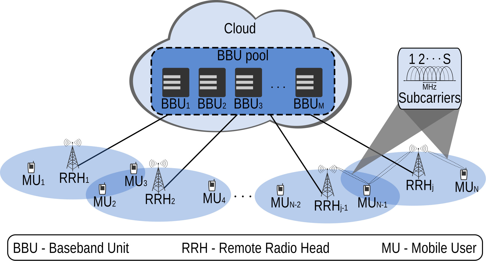 Figure 1
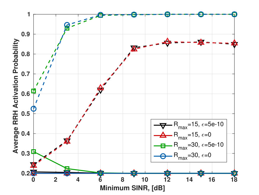 Figure 10
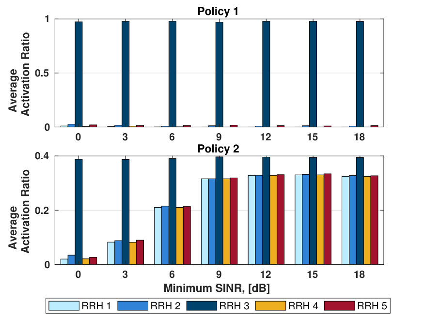 Figure 11
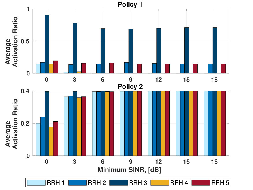 Figure 12
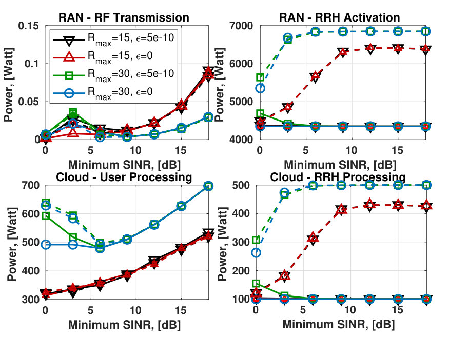 Figure 13
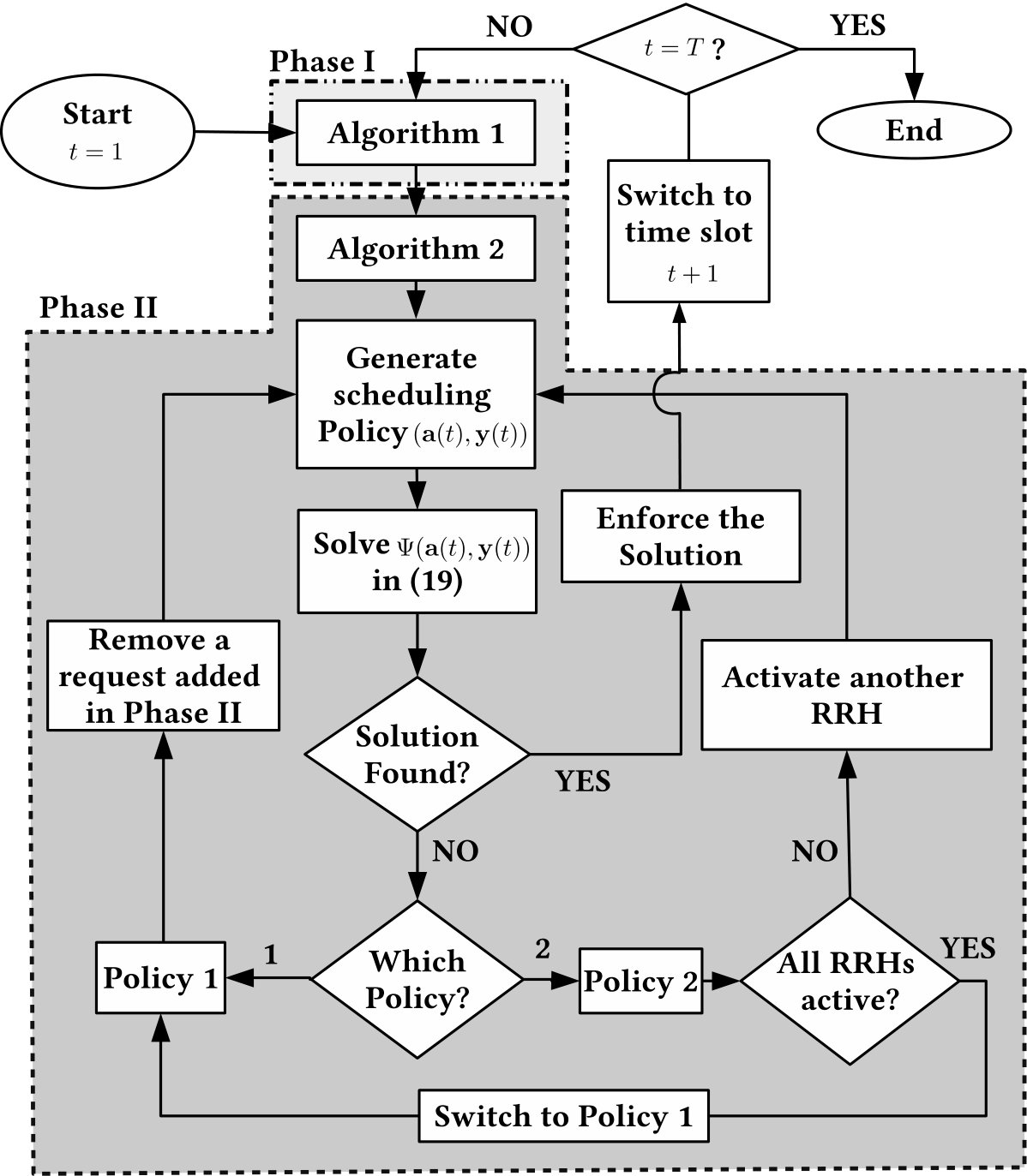 Figure 2
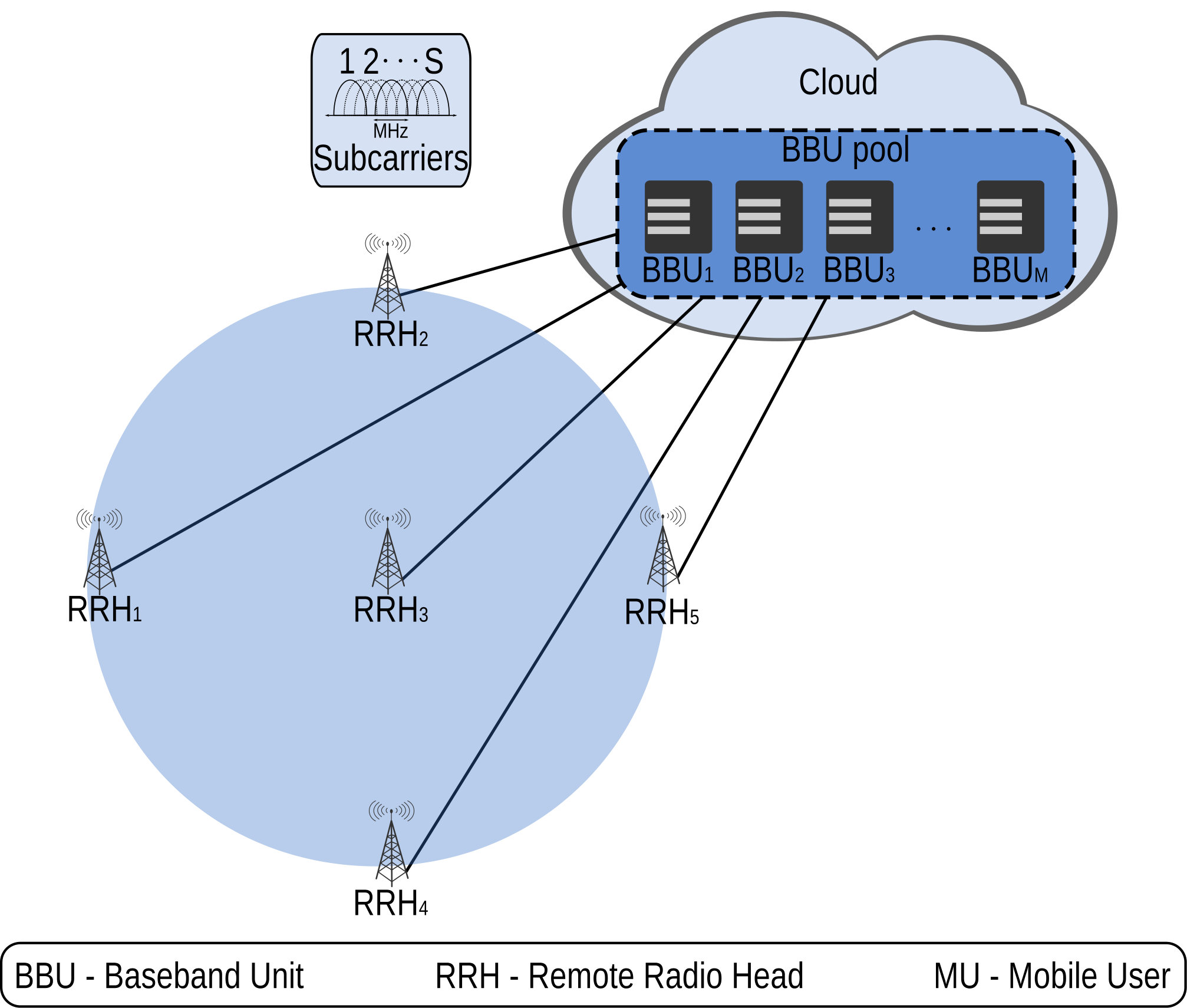 Figure 3
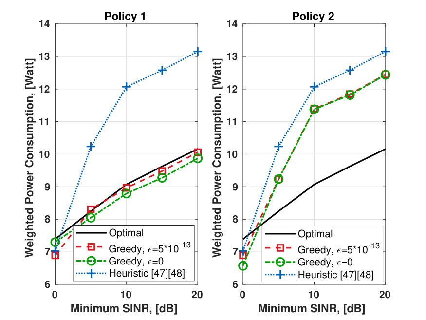 Figure 4
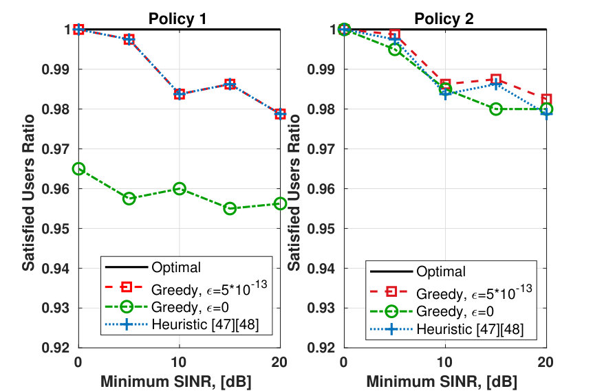 Figure 5
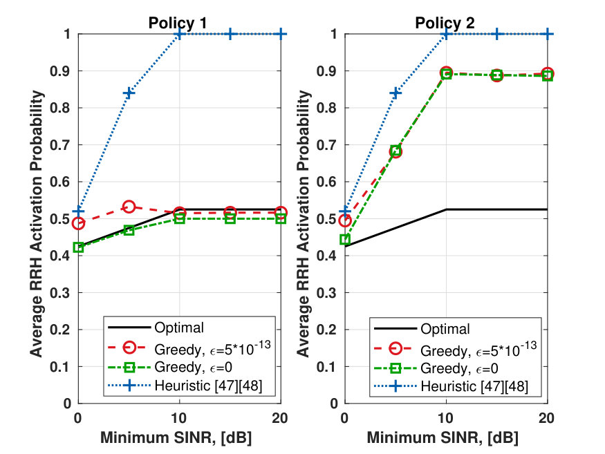 Figure 6
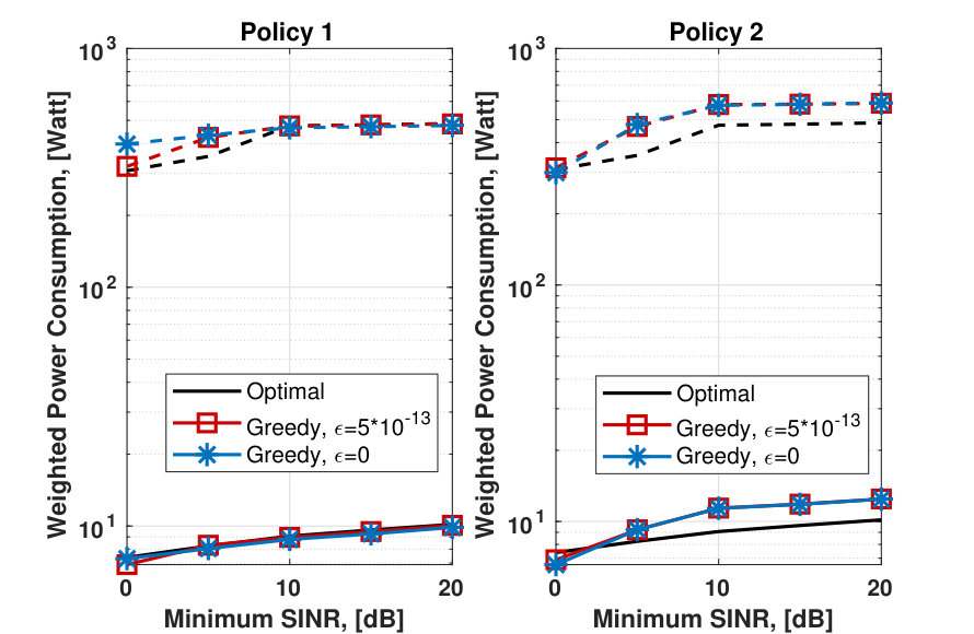 Figure 7
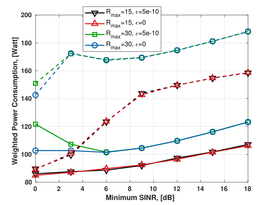 Figure 8
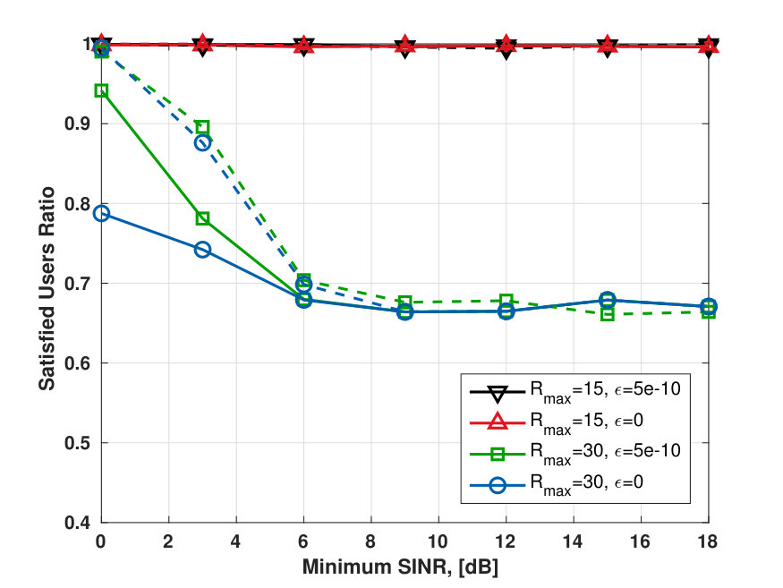 Figure 9
 Figure 15
 Figure 16
 Figure 17
 Figure 18
| Variable | Description |
|---|---|
| , , , | Sets of users, RRHs, subcarriers and requests |
| Maximum transmission power level of an RRH | |
| Arrival time of a request and its deadline | |
| Amount of computational resources to process a request | |
| Channel gain matrix | |
| Noise power on each subcarrier | |
| Horizon duration | |
| Minimum average SINR requirement | |
| Allocation variable | |
| Activation indicator | |
| Transmission power level | |
| Computational resources of the BBU pool | |
| Fibers, activation and sleep power costs | |
| Consumed power by the BBU pool when resources | |
| are allocated | |
| Transmission, activation and total power costs | |
| Total processing power cost in the BBU pool | |
| Overall weighted power consumption of the network | |
| Weighting parameters |
| 0 dB | 5 dB | 10 dB | 15 dB | 20 dB | |
|---|---|---|---|---|---|
| Case A | 0.402 | 0.421 | 0.553 | 0.562 | 0.611 |
| Case B | 0.324 | 0.375 | 0.449 | 0.511 | 0.525 |
Peer Reviews
No public reviews on file for this paper yet. If you reviewed it on a platform where reviews are public (OpenReview, ICLR, NeurIPS, ICML), you can paste yours below so the community can read it here.
Videos
No videos yet. Explain this paper in a talk, walkthrough, or lecture? Add one.
Power-Efficient Resource Allocation in C-RANs with SINR Constraints and Deadlines
Salvatore D’Oro, Marcelo Antonio Marotta , Cristiano Bonato Both , Luiz DaSilva, Sergio Palazzo Copyright (c) 2015 IEEE. Personal use of this material is permitted. However, permission to use this material for any other purposes must be obtained from the IEEE by sending a request to [email protected]. D’Oro is with the Institute for the Wireless Internet of Things, Northeastern University, Boston, USA, email: [email protected];S. Palazzo is with the Dipartimento di Ingegneria Elettrica, Elettronica e Informatica, CNIT Research Unit, University of Catania, Italy, email: [email protected];M. A. Marotta is with the University of Brasilia, Brazil, email: [email protected];Cristiano B. Both is with the Applied Computing Graduate Program at University of Vale do Rio dos Sinos (UNISINOS), Brazil, email: [email protected];L. DaSilva is with the CONNECT Research Centre at Trinity College Dublin, Ireland, email: [email protected] work was partially supported by the Science Foundation Ireland under grant number 13/RC/2077, SFI Research Centre CONNECT.
Abstract
In this paper, we address the problem of power-efficient resource management in Cloud Radio Access Networks (C-RANs). Specifically, we consider the case where Remote Radio Heads (RRHs) perform data transmission, and signal processing is executed in a virtually centralized Base-Band Units (BBUs) pool. Users request to transmit at different time instants; they demand minimum signal-to-noise-plus-interference ratio (SINR) guarantees, and their requests must be accommodated within a given deadline. These constraints pose significant challenges to the management of C-RANs and, as we will show, considerably impact the allocation of processing and radio resources in the network. Accordingly, we analyze the power consumption of the C-RAN system, and we formulate the power consumption minimization problem as a weighted joint scheduling of processing and power allocation problem for C-RANs with minimum SINR and finite horizon constraints. The problem is a Mixed Integer Non-Linear Program (MINLP), and we propose an optimal offline solution based on Dynamic Programming (DP). We show that the optimal solution is of exponential complexity, thus we propose a sub-optimal greedy online algorithm of polynomial complexity. We assess the performance of the two proposed solutions through extensive numerical results. Our solution aims to reach an appropriate trade-off between minimizing the power consumption and maximizing the percentage of satisfied users. We show that it results in power consumption that is only marginally higher than the optimum, at significantly lower complexity.
Index Terms:
Cloud Radio Access Networks, resource allocation, energy efficiency.
I Introduction
Cloud Radio Access Networks (C-RANs) are expected to provide unprecedented scalable, flexible, and efficient infrastructure provisioning and management in future 5G networks and beyond [1, 2, 3]. In Cloud Radio Access Networks, a set of Remote Radio Heads perform radio transmissions, while signal processing, *e.g., *base band processing, is executed in a pool of one or more Base Band Units as a cloud system [4, 5, 6]. RRHs and BBUs are interconnected through high-speed optical fiber links, which makes it possible to meet the high-performance requirements of 5G networks, thus guaranteeing low latency and high-rate data transmission [7].
C-RANs can achieve a considerable reduction of both CAPEX and OPEX while providing efficient and smart management of network resources. Since the signal processing is performed in the BBU pool, the RRHs are characterized by a simple transceiver design. In addition, by exploiting the centralized architecture of the BBU pool, it is possible to perform advanced and efficient signal processing techniques that require coordination. For example, Coordinated Multipoint (CoMP) and Joint Transmission (JT) can be implemented to reduce interference and improve the spectral efficiency of the system. To process a given user transmission in C-RAN environments, the system: i) allocates the user to the available downlink channels; ii) selects the subset of active RRHs which will transmit to the corresponding user, and determines the transmission power level of those RRHs; and iii) runs a Virtual Function (VF) [8], or creates a Virtual Machine (VM) [9] instance in the BBU pool, to which a given amount of computational resources is assigned. In the remainder of this paper, we do not distinguish between virtual functions and virtual machines, and we refer to both of them as VMs.
To take full advantage of C-RANs, green and lightweight management of network resources has to be considered [10]. However, C-RANs comprise heterogeneous network elements, which makes the design of energy-efficient algorithms a challenging task. As an example, to minimize the power consumption of the whole C-RAN system, both radio and computational resources must be managed jointly. That is, the activation and management of RRHs have to be addressed together with the efficient allocation of the computational resources in the BBU pool. This problem is not trivial, and it is further exacerbated when minimum Quality of Service (QoS) requirements, such as temporal deadlines and Signal-to-interference-plus-noise ratio (SINR), are considered [11]. Due to its complexity and importance, many solutions to the green management of C-RANs have been proposed in the literature [12, 13, 14, 15, 16, 9, 17, 18, 19, 20]. However, those solutions have not been designed to deal with the relevant case of finite-horizon scheduling problems. Thus, they are expected to be sub-optimal when user transmission requests dynamically arrive at different time instants and have to be accommodated within a given deadline.
In this paper, we design an optimal green mechanism for such a dynamic scenario. Specifically, we analyze the case where subscribers dynamically submit transmission requests, coupled with the corresponding requirements regarding minimum average SINR and a delivery deadline. We formulate the power consumption minimization problem for C-RANs as a weighted joint power allocation and user scheduling problem. By considering that the BBU pool has limited computational resources, we account for both temporal and SINR constraints, and we show that the problem can be formalized as a Mixed Integer Non-Linear Problem (MINLP). For such a problem, we provide an optimal offline solution based on Dynamic Programming (DP) techniques. We show that its computational complexity is exponential, which makes it unfeasible to obtain an optimal solution in large-scale and dense networks within a reasonable amount of time. Accordingly, we design a greedy online algorithm of polynomial computational complexity. We assess and compare the performance of the two proposed solutions through extensive numerical results. Our solution aims to reach an appropriate trade-off between minimizing the power consumption and maximizing the percentage of satisfied users. Our proposed algorithm results in power consumption that is only marginally higher than the optimum, at significantly lower complexity.
The remainder of this paper is organized as follows. Related work is presented in Section II. Section III illustrates the considered C-RAN, and the corresponding power consumption analysis. The weighted joint power allocation and user scheduling are formulated in Section IV. Section V provides the optimal offline solution to the problem. A sub-optimal online solution with polynomial complexity is proposed in Section VI. Numerical results are presented in Section VII. Finally, in Section VIII we outline our main conclusions.
II Related Work
The problem of providing power-efficient 5G systems under QoS constraints through joint user transmission scheduling and power allocation has been extensively addressed in the literature. As an example, the downlink joint power and wireless resource allocation problem in C-RANs under minimum SINR constraints has been considered in [12, 13, 14, 15, 16]. In [9], a cross-layer approach for the power-efficient allocation of network resources is considered where both the RRHs and the BBU pool are assumed to have limited computational and hardware resources. The same problem is also addressed and solved in [17] where, instead, a requirement on the desired task completion time is considered. A different approach is contemplated in [18], where power control and caching at the RRHs are exploited to provide mobile users with minimum QoS guarantees. In contrast, a fractional programming approach is proposed in [19] to maximize the energy efficiency of the network. Those works focus on minimizing the actual overall power consumption of the network. However, it is worth noting that the consumed power of each network element can be significantly different. As an example, the power needed to activate the optical fibers between the BBU pool and the RRHs can be significantly lower than the power needed to activate the RRHs [20]. Accordingly, a more general approach consists in the minimization of a weighted version of the actual power consumption. Such an approach is considered in [21], where the weighted power consumption of the network is minimized by jointly addressing the power and resource allocation problems for both downlink and uplink communications.
Though optimal, most of the above solutions do not consider limited computational resources at the BBU pool. Furthermore, they have not been designed to deal with finite-horizon scheduling problems, where user transmission requests dynamically arrive and have to be scheduled within a deadline. The scheduling problem for C-RANs over a finite horizon has been considered in [22, 23]. However, the solution in [22] only focuses on the BBU pool and does not consider the power consumption of the RRHs, while [23] does not account for CoMP transmissions, and the power consumption is restricted to the transmission power only.
The above literature review reveals that the problem of minimizing the power consumption of C-RANs over a finite-horizon through joint RRH and BBU management is worth investigating. It also shows that further efforts are needed, as none of the above solutions can be readily applied to optimally solve the finite-horizon power minimization problem we consider in this paper.
III System Model
We study a C-RAN scenario where mobile users access the network using several RRHs which are connected to a BBU pool through high-speed optical links, as shown in Fig. 1. We consider a a time slotted multi-carrier (or multi-frequency) system where a set of subcarriers are available for data transmission.
In this work, we focus on the downlink communications between RRHs and mobile users. We assume that the allocation of downlink resources has to be performed over a finite horizon. The finite-horizon concept captures time requirements in those scenarios where channel gain coefficients or user positions change every slots (*e.g., *slow-fading or block-fading scenarios). Let denote the set of time slots within the horizon.
III-A Modeling Mobile Users
Let be the set of mobile users in the network. One or more RRHs can serve each user . In the following, we assume that mobile users are equipped with single-antenna transceivers, which at any given time instant can only receive signals on a single subcarrier.
Each user transceiver generates one (or more) request-to-transmit to the Telecommunications Operator (TO). Specifically, each request contains the following parameters:
- •
Requesting User: it is the mobile user who sends the request .
- •
Deadline: mobile users’ requests have to be accommodated by 1) instantiating a VM in the BBU pool to process user signals; and 2) scheduling downlink transmissions through one (or more) RRHs for the whole duration of a time slot [9] within a given temporal window. For each request, the temporal window is defined by the 2-tuple , where represents the arrival time slot of the request, and is the duration of the temporal window within which the request must be accommodated.
- •
SINR Constraint: it represents the minimum average SINR level that has to be guaranteed to request .
- •
Computational Resources: they represent the amount of computational resources to run a VM in the BBU pool for request . In general, the higher the value of , the higher the value of , i.e., with . Such an assumption stems from the evidence that large values of require the BBU pool to run more complex signal processing operations. Accordingly, can be modeled as follows [24, 25]:
[TABLE]
where is a constant term that represents the amount of resources needed to activate a VM and perform signal processing (*e.g., *modulation, encoding, Fast Fourier Transform, etc..), and is a weighting parameter to vary the slope of the function [25]. It is worth noting that (1) quantifies the amount of computational resources in the BBU pool to be allocated to a given request that demands a minimum SINR level . How to satisfy the aforementioned SINR requirement will be the main topic of Sections V and VI, where joint power and channel allocation is effectively used to satisfy users’ requests while minimizing the power consumption of the system.
- •
Channel State Information (CSI): at each time slot , the channel is modeled through its channel coefficient , which represents the channel between the mobile user who has made the request and the RRH on subcarrier at time slot . For clarity of notation, we introduce the channel gain coefficient . Accordingly, the CSI is represented by the channel gain coefficient matrix . We assume block-fading, *i.e., *channel gain coefficients remain constant within each time slot .
Without loss of generality, in the following we omit the time slot indicator and we focus on the case where channel gain coefficients do not vary within the horizon, i.e., for all . However, the solutions proposed in this paper also apply to the more general case where channel gain coefficients vary at each time slot. Accordingly, each request is defined by the 6-tuple . Also, we assume that CSI information is always available to the system through pilot-based [26, 27] or statistical [28, 29] approaches. However, we do not make any assumption on the accuracy of the CSI estimation procedure.
III-B Modeling RRHs
RRHs are equipped with multiple antennas and are capable of performing simultaneous transmissions on multiple subcarriers. However, due to hardware limitations, RRHs are required to satisfy a power constraint. Specifically, at each time slot , the total transmission power for each RRH has to be lower than or equal to an RRH-specific maximum transmission power level . RRHs are connected to the BBU pool through high-speed optical fiber links.
III-C Modeling the BBU pool
The BBU pool is the centralized entity where signal processing is performed. Through centralized processing, it is possible to exploit advanced signal processing techniques such as CoMP and JT. Hence, to improve the SINR and reduce the interference with other mobile users connected to adjacent RRHs, in this work we exploit both techniques to provide JT-CoMP transmissions where several RRHs simultaneously transmit the same signal to a given user. When a given request is scheduled, a VM instance on the BBU pool is instantiated, and a given amount of computational resources in the pool is assigned to it. Specifically, for each request the system: 1) allocates a downlink time slot on a given subcarrier to the corresponding mobile user; 2) selects the subset of active RRHs which will transmit to the corresponding mobile user, and determines their optimal transmission power levels; and 3) creates a VM instance in the BBU pool. Also, we assume that the BBU pool has a limited amount of computational resources.
III-D Variables Definition
We hereby introduce the relevant variables in our model of the C-RAN scenario, which for the sake of clarity are also summarized in Table I. Let be the set of all the requests sent by mobile users. To model the allocation of mobile users in the time and frequency domains, we define the allocation variable , where if request is allocated to sub-carrier at time slot . Otherwise, . Let , where . Furthermore, the transmission power of RRH on subcarrier at time slot is defined as the continuous variable . Let , where .
To model the selection (*i.e., *activation) of an RRH, we define the following activation indicator , where if RRH is transmitting at time slot . Otherwise, . Let , where .
Accordingly, for each and , the average SINR can be written as follows:
[TABLE]
where is the noise power on the considered subcarrier, and is the expected channel gain coefficient w.r.t. the mobile user which requested and the RRH on subcarrier .
III-E Constraints Definition
Under the above assumptions, we define the following constraints:
RRH power constraint: for each activated , the overall transmission power has to be lower than . Thus,
[TABLE] 2. 2.
Scheduling constraints: each mobile user has a single antenna, thus it can be scheduled to a single subcarrier. Also, its request has to be accommodated only once. Furthermore, a given request cannot be scheduled if its corresponding temporal requirement is not satisfied. That is,
[TABLE]
Furthermore, and if . 3. 3.
SINR Constraint: the average SINR for each scheduled mobile user defined in (2) has to be higher than the minimum QoS requirement
[TABLE] 4. 4.
BBU bounded computation constraint: the amount of computational resources in the BBU pool is, in general, bounded. Let be the maximum amount of computational resources which are available in the BBU pool. Accordingly, at each time slot we have that the amount of resources allocated to requests in is bounded by . From constraint (4), this constraint can be defined as follows:
[TABLE]
III-F Power Consumption
In the considered scenario, the main sources of power consumption can be summarized as follows:
- •
RRH Transmission and Activation: at the RRH side, there are three main power-consuming processes. First, each RRH that has been selected for data transmission has to be turned on. Accordingly, there is an activation power cost equal to . Second, when an RRH is turned on, it is also connected to the BBU pool through optical fibers, which generates a fiber power cost equal to . Note that depends on as RRHs are located at different distances from the BBU pool. RRHs which are far away from the BBU require optical amplifiers, additional connectors and fibers. Therefore, their will be larger, while nearer RRHs will have a small . The third process is represented by the transmission power levels .
It is worth mentioning that the switch between on/off states would be too costly at small time-scales (e.g., data frame scale). In fact, RRHs can not be instantaneously turned on due to hardware constants, which eventually results in processing and transmission latency that might not be acceptable for small-scale and fast-varying networks [30]. For this reason, and for the sake of generality, we adopt a general model where RRHs can be either completely turned off or put in a sleep state [30]. Accordingly, the power consumption at time slot for RRH can be expressed as follows:
[TABLE]
where is a non-negative parameter to weigh the two contributions in (7), and
[TABLE]
where is the power consumption of the RRH when it is put in a sleep state [31, 32]. It is worth mentioning that such an approach is general and also allows us to account for a broader range of applications [30]. From (7), the total power consumption for all RRHs at time slot can be written as
[TABLE]
- •
BBU Allocation: for each scheduled mobile user, a VM has to be instantiated in the BBU pool. Also, to provide the desired SINR level to each request , computational resources must be assigned to a VM. Accordingly, the power consumption to process request at the BBU pool can be expressed as follows:
[TABLE]
where is the per resource power consumption. Thus, the overall power consumption at the BBU pool side at time slot is .
Accordingly, we have that the total weighted power consumption in the network at time slot is defined as follows:
[TABLE]
where is a non-negative parameter used to weigh the power consumption at both the RRH and BBU sides. Accordingly, the total weighted power consumption of the C-RAN system within the considered time window is
[TABLE]
Remark 1*.*
The above analysis clearly shows that the power consumptions at both RRH and BBU sides are tightly coupled. In fact, wireless transmissions in C-RAN systems not only require the allocation of a given amount of transmission power on each RRH, but they also rely on the instantiation of VMs and the allocation of computational resources in the BBU pool. It follows that efficient power management in C-RAN systems requires jointly reducing the power consumption of all network elements in the cloud and the Radio Access Network (RAN). We would also like to point out that the complexity and importance of such a power minimization problem is further exacerbated in the considered finite-horizon scenario, where optimal request scheduling is essential to guarantee low power consumption in the network. This motivates our work, whose objective is to design optimal resource allocation mechanisms that effectively minimize the power consumption of a C-RAN system over a finite-horizon while satisfying both SINR and scheduling constraints.
IV Problem Formulation
The problem of finding an optimal allocation of network resources at both the RRH and BBU sides that minimizes the weighted power consumption while satisfying user requirements and system constraints, can be formulated as Problem .
[TABLE]
where ; ; and .
The power constraint is enforced by Constraint (3). Constraint (4) ensures that each request is accommodated exactly once, and each user is scheduled to only one of the available subcarriers. The SINR constraint is defined by the non-linear Constraint (5), and Constraint (6) prevents the system from allocating more computational resources than those available in the BBU pool. Finally, Constraints (14), (15), (16) and (17) guarantee the feasibility of the solution.
V Optimal Offline Solution
Problem aims at reducing the weighted power consumption of the system while jointly: i) allocating requests to the available sub-carriers, ii) activating VMs in the BBU pool and assigning computational resources according to (1), iii) selecting the subset of active RRHs, and iv) controlling their transmission power to satisfy QoS requirements. In more detail, Problem is formulated as an MINLP which is well-known to be NP-hard.
Specifically, Problem is combinatorial, and an exhaustive search approach would result in exponential time solutions whose application to realistic scenarios is unfeasible. To overcome the above issues, and to reduce the complexity of the optimal solution, we propose the exploitation of Dynamic Programming (DP) techniques. In the remainder of this paper, we assume that a feasible solution to Problem exists. However, the existence of a solution can be verified by executing a feasibility test.
In the language of DP, we define:
- •
System state: at each time slot , the state of the system is defined as the set of active requests that have not yet been accommodated. Specifically, we have that ;
- •
Action: at each time slot , we need to find the optimal scheduling policy , the subset of active RRHs to serve those requests, and the transmission power profile . Accordingly, the actions to be taken can be defined as the 3-tuple ;
- •
Single Slot Reward: the single slot reward consists in the single slot weighted power consumption in (12).
Accordingly, to solve the problem through DP, for each time slot , we write the Bellman’s equation [33] as
[TABLE]
where for all , and
[TABLE]
where, for any given tuple , , , and .
From (2), we have that the SINR constraint in problem is non-linear. However, the same constraint can be expressed through the equivalent linear inequality
[TABLE]
Since the problem is a minimization one, it is straightforward to show that the SINR constraint is an active constraint, *i.e., *the optimal solution of the problem implies that the SINR constraint in (V) must be met with equality. Accordingly, the problem can be restated as a Linear Programming (LP) one. Specifically, it can be easily shown that the objective function and all constraints in are convex functions. Therefore, the LP problem is also convex, and any feasible local minimum solution is also a global solution to the problem. For any given tuple and time slot , we solve the single-stage power control problem by using standard interior-point or simplex methods.
By exploiting DP, it is possible to obtain the optimal solution to the weighted power consumption minimization problem. Specifically, at each stage, we consider all possible combinations of the outstanding request set . Then, we consider all possible combinations of . For any given combination , we solve the power allocation problem which is LP and can be solved with polynomial complexity. Instead, the single slot optimization problem in (V) is an Integer Linear Programming (ILP) problem which can be solved through the branch and bound approaches whose worst-case computational complexity equals that of exhaustive search algorithms. Finally, we exploit backward induction [33] to solve the Bellman’s equation and find the optimal solution of the problem.
Let be the maximum number of requests in the system. The number of combinations of the outstanding request set is . The number of combinations of and are and , respectively. Thus, the single slot optimization problem in the Bellman’s equation has complexity . Let be the complexity of the power control problem. The overall complexity of the finite-horizon power consumption minimization problem over slots is . That is, finding the optimal solution of the considered problem results in exponential computational complexity.
VI Online Greedy Algorithm
The offline solution in Section V is designed to obtain an optimal solution of Problem . However, it does not scale well with the number of variables in the problem and requires a priori knowledge of all the requests submitted by all network users. Accordingly, to obtain an optimal solution in large-scale and dense networks within a reasonable amount of time is unrealistic. Also, requests submitted by network users are expected to arrive in real-time and are not available in advance. Therefore, alternative online approaches must be considered.
At any given time instant , is the set of outstanding requests. For the sake of readability, in the following, we omit the time slot index . It is worth noting that network nodes dynamically submit a request and no information concerning their arrival time and minimum SINR requirements is available. In such an uncertain scenario, optimality should be relaxed, and a sub-optimal solution needs to be considered. For these reasons, in this section, we propose a sub-optimal online algorithm which can be implemented with polynomial time complexity.
As shown in Fig. 2, the proposed greedy algorithm comprises two phases. Phase I is devoted to the computation of a greedy orthogonal scheduling policy that accounts for deadline constraints and limits to zero (or to a small constant factor) interference among users. Phase II is devoted to the exploitation of JT and spectrum sharing to schedule additional requests while satisfying users’ requirements. The technical details of Phase I and Phase II are described in Subsections VI-A and VI-B, respectively.
VI-A Phase I: Greedy Orthogonal Scheduling
Let , and , where is a parameter whose importance w.r.t. the proposed greedy algorithm will be described in Step I.4 in this subsection. For each , and , we define the following parameters
[TABLE]
At each time slot , is the waiting time (or queueing time) of request . That is, indicates the number of time slots that request spent inside the BBU pool queue without being scheduled. represents the minimum amount of power to fulfill the minimum average SINR level requirement of request on channel when served by RRH without any other interfering transmission. Intuitively, smaller values of , *i.e., *loose SINR requirements, and high channel gain coefficients , *i.e., *better channel conditions, lead to lower transmission power requirements . Conversely, poor channel quality and high SINR requirements lead to larger values of .
The algorithmic procedure of Phase I is summarized in Algorithm 1 and it is described in the following.
- •
Step I.1: For each , we define . We also generate with
[TABLE]
Intuitively, (23) has high values when the request : i) requires a small amount of transmission power to meet the SINR constraint; and ii) already spent several time slots in the system without being scheduled. In this step, we sort in ascending order. The obtained ordering is then used to sort 111Note that this step is not the same as simply ordering in ascending order as the two resulting orderings are generally different.. This approach generates an ordering of where requests that are approaching their deadline are prioritized. Conversely, the scheduling of requests that are still far away from their deadline is delayed in time. This strategy is known in the literature as Earliest Deadline First (EDF) [34], and it has been successfully utilized many times to design efficient greedy algorithms [35, 36]. The rationale behind (23) is twofold, as priority is given to those requests that i) are approaching their deadline and ii) require the least amount of power to satisfy their minimum SINR requirement. Recall that any unscheduled request makes the Constraint (4) unsatisfied, and thus generates an unfeasible solution to Problem . Also, requests associated to low values of are the ones that require lower transmission power to satisfy their minimum SINR requirement. Accordingly, the ordering generated through (23) jointly aims at minimizing the objective function of Problem and enforcing Constraint (4).
- •
Step I.2: For each , we build a greedy scheduling policy as follows. We consider only those requests which require the lowest transmission power to be satisfied, while guaranteeing that bounds the overall transmission power. That is, we schedule those requests in with the smallest in , such that . We assume that each RRH can assign a channel to no more than one request at a time. Furthermore, from (4), we have that each request can be scheduled on no more than one channel. Therefore, from the orthogonality assumption, in there could not be two requests sharing the same channel, and each request can appear only once.
- •
Step I.3: We pick the RRH which schedules the highest number of requests with the lowest power consumption. That is, we select such that . Ties are broken by selecting the RRH such that the overall power consumption is minimum, i.e., . We add to , i.e., .
- •
Step I.4: Let be the RRH selected at Step I.3. We build a candidate greedy scheduling policy such that . Then, we consider
[TABLE]
which we define as the -orthogonal set of RRHs whose interference to the scheduling in is upper-bounded222Recall that when is served by RRH on channel , the interference at is , where represents the transmission power of an interfering RRH on channel . In this case, . Thus, we can effectively limit the experienced interference at by a factor proportional to by allowing transmissions from any RRH such that . by a small multiple factor of . Intuitively, if , it means that transmissions performed by RRHs in do not interfere with the scheduling . Instead, small positive results in small tolerable interference values.
- •
Step I.5: Requests already in are removed from , i.e., . Also, the set of orthogonal RRHs is updated such that . Then, Step I.2 is iteratively re-executed among the remaining RRHs in , and the best RRH in is selected again until or no more requests can be scheduled as there are no more computational resources in the BBU pool. That is, .
VI-B Phase II: JT and Channel Sharing Scheduling
For each RRH , let be the scheduling policy at the end of Phase I. Accordingly, for each RRH we calculate its residual power under policy as follows:
[TABLE]
and we define as
[TABLE]
Intuitively, is the subset of activated RRHs whose residual power is positive at the beginning of Phase II. Such residual power can be used to schedule multiple user transmissions on the same channel on the same RRH, or to perform JT operations through multiple RRHs that transmit to the same user. To this end, in the following we first derive a scheduling policy . At the beginning of Phase II, is empty, of course. Then, we use to derive a joint user scheduling and power allocation strategy .
The computation of is described in the following. For the sake of clarity, the same procedures are also illustrated in Algorithm 2.
- •
Step II.1: We select the request which corresponds to the minimum required transmission power and can be scheduled by exploiting the residual power of the RRHs in . Specifically, we select such that
[TABLE]
- •
Step II.2: We update the Phase II scheduling policy .
- •
Step II.3: We remove from the outstanding requests set, i.e., .
- •
Step II.4: We update the residual power of as follows: . If , we remove from .
- •
Step II.5: Step II.1 is iteratively re-executed as soon as one of the following conditions is satisfied: i) all the residual power has been exhausted, i.e., ; ii) the set of outstanding requests is empty, i.e., ; iii) no more requests can be processed in the BBU pool, i.e., for all .
Let be the scheduling policy obtained at the end of Phase I and Phase II, where , and .
We set for all the scheduled requests such that , and we set for those activated RRHs . Thus, at each time slot , we obtain the RRH activation vector and the request scheduling matrix . Those two variables are used to compute and to solve the power minimization problem in (V). If a solution is found, the resulting scheduling and transmission policy is enforced. Otherwise, if no solution exists, two alternative approaches can be followed. Specifically, we can either i) unschedule the extra requests, or ii) activate an additional RRH to search for a feasible power control solution. Those two approaches can be summarized in the two following policies:
Policy 1: We solve the power control problem (V) by iteratively removing the requests in whose required minimum transmission power is maximum until a solution is computed. If the requests in are all removed, then the original orthogonal scheduling is found. Accordingly, if , a solution to the problem (V) must exist by the construction of the greedy orthogonal scheduling policy . Otherwise, if and a solution to (V) does not exist, then we set and we re-execute Phase I, which surely admits a solution. 2. 2.
Policy 2: We iteratively launch the power control algorithm by iteratively activating the least power consuming RRH in until we find a feasible solution. If all RRHs have been activated and no solutions are found, then we launch Policy 1 until a feasible solution is obtained.
For illustrative purposes, in Fig. 2 we present the block diagram corresponding to the proposed greedy algorithm when . It is worth noting that if a solution is found, the algorithm enforces the obtained scheduling policy and moves to the next time slot. The block diagram for the case where is similar to that shown in Fig. 2. The only difference is that if no solutions are found at the end of Policy 2 and Policy 1, then the algorithm is re-executed by setting , which, at least, ensures that Phase I generates an orthogonal greedy scheduling policy.
The complexity of the ordering in Step I.1 is . The operation is performed times. Therefore, Step I.1 has complexity . Steps I.2 – I.5 have complexity . However, they are iterated over all the available RRHS until a greedy orthogonal scheduling policy is obtained. Accordingly, they have complexity , and Phase I has overall complexity . Similarly, it can be shown that Phase II has complexity . Policy 1 has complexity , while Policy 2 has complexity . Therefore, the overall complexity of the proposed greedy algorithm is .
VII Numerical Analysis
In this section, we assess the achievable performance of the above proposed solutions through extensive numerical simulations. Specifically, in Section VII-A we analyze the performance of the optimal solution. The achievable performance of the proposed greedy scheduling algorithm is discussed in Section VII-B.
Our study not only focuses on the power consumption of the C-RAN system under the algorithms proposed in the previous Sections, but it also investigates two relevant metrics, namely satisfied user ratio and RRH* activation probability*. The former indicates the percentage of users whose requests are satisfied by the network. The latter gives us important information on the number of RRHs that must be effectively turned on to support user data transmissions and guarantee minimum SINR requirements.
To assess the performance of the proposed solutions, we consider a circular network scenario. Despite its simplicity, this model has been identified as a good candidate for performance evaluation in C-RAN systems, and has been effectively used many times in the literature [9, 37, 38, 39, 40, 41] as a benchmark for power allocation, user scheduling, and resource allocation algorithms. In our simulations, we assume that RRHs and a BBU pool are deployed in a circular area as shown in Fig. 3. The corresponding fiber power costs , which depend on the distance between the BBU pool and the RRHs, are W. Let us point out that our solution is general and can be utilized independently of the actual distribution of users in the network. However, for simulation purposes only, we model the position of network users as a random variable with circular uniform distribution [24, 42, 43]. Specifically, at each simulation run, the position of network users is randomly generated within a circle whose radius is set to m. Channel gain coefficients are generated according to the path-loss model in [44] for Rayleigh fading channels. The activation and sleep power costs are assumed to be equal for all the RRHs. Specifically, we set W [45, 31] and W [31]. The maximum transmission power level for each RRH is set to dBm [45]. We consider the case where the amount of computational resources to process each request increases linearly with the achievable Shannon capacity, i.e., the slope in (1) is set to . Also, we assume that the amount of computational resources to process data requests in the BBU pool is . Accordingly, we have for all , which yields for all . We assume that such a cost is W. The weight parameters are set to and . Finally, we assume that users submit their requests according to a binomial distribution [46] with success probability , and the number of trials equal to , where represents the maximum number of users in the network. The results shown in this subsection are averaged over 5000 simulation runs.
VII-A Optimal Offline Solution
In this subsection, we assess the performance of the optimal offline solution proposed in Section V, and we compare it with other scheduling policies. As already discussed in Section V, to find an optimal solution to the joint scheduling and power allocation problem is a NP-hard problem, *i.e., *it has exponential complexity in the number of variables of the problem, which makes it infeasible to compute an optimal solution even for small network instances. Thus, in this section only, we restrict our performance evaluation to the case where only and can be activated, while the remaining RRHs are switched off333The case where all RRHs can be selected will be extensively investigated in Section VII-B.. Furthermore, we consider a system where subcarriers are available for data transmission. The optimization horizon is set to , and we assume that all requests have to be accommodated before the horizon is reached. Finally, we assume that number of users in the network is .
In Fig. 4, we show the weighted power consumption in (13) as a function of the minimum average SINR requirement level and the parameter in (24). Specifically, we compare the optimal offline solution (solid lines) with two other algorithms: the greedy online algorithm proposed in Section VI (dashed lines), and the heuristic approach considered in [47] and [48] where all RRHs are turned on simultaneously when there is at least one request to be served (dotted lines). In general, the power consumption always increases as the minimum average SINR requirement level increases. Also, the power consumption under the optimal policy is generally lower than that achieved by all the other considered algorithms. It is worth noting that Fig. 4 shows some cases where the power consumption of the network under the greedy algorithm is lower than that achieved when the optimal solution is considered. This result is explained in Fig. 5, where we show that the above phenomenon arises in those cases where the greedy algorithm does not produce a feasible solution that satisfies the minimum SINR constraints, *i.e., *when some requests cannot be satisfied. By reducing the number of served users, the corresponding power consumption is also reduced, thus explaining why the greedy algorithm shows lower power consumption in some cases. As expected, when all requests are satisfied, *i.e., *the satisfied users ration is equal to 1, the optimal algorithm always provides the best performance. It is also worth noting that Policy 1 achieves near-optimal performance if compared to the optimal solution, and the additional cost introduced by the greedy algorithm is small, and anyway lower than that introduced by the heuristic approach. Although Policy 1 slightly under-performs Policy 2 in terms of satisfied users ratio, it both achieves very high satisfaction percentage, (i.e., 96% of the total number of users) and also consumes less power than Policy 2. For network operators, the combination of the greedy algorithm and Policy 1 presents an opportunity to save energy in those scenarios where the minimum SINR requirement is low. Instead, when high SINR levels are required, the greedy algorithm with Policy 2 should be preferred.
To better understand the motivation behind the above findings, in Fig. 6 we show the average activation percentage of the two RRHs for the three algorithms as a function of the minimum average SINR requirement level. It is shown that the optimal solution (solid lines) activates the lowest number of RRHs, thus resulting in low power consumption levels. On the contrary, both the proposed (dashed lines) and the heuristic (dotted lines) approaches activate a higher number of RRHs. Specifically, since the heuristic approach activates all the RRHs when at least one request has to be scheduled, it results in the highest power consumption. Instead, the activation percentage under the proposed greedy algorithm under Policy 1 is slightly higher than that achieved under the optimal policy. For C-RANs composed of RRHs with high energy activation cost, Policy 1 brings even further energy consumption benefits considering the aforementioned trade-off regarding users’ satisfaction. Whereas, when Policy 2 is used, the system will benefit from near optimal user satisfaction with better energy consumption than previously proposed solutions, such as the heuristic in [47, 48].
It is worth noting that the average RRH activation probability for the heuristic approach (dotted lines) is not always equal to . Such a result is due to the fact that the heuristic approach activates all the RRHs if and only if there is at least one request to be scheduled. Otherwise, the RRHs remain inactive. Furthermore, the power consumption generated by the proposed greedy algorithm under both Policy 1 and Policy 2 increases as the minimum SINR level increases as well. As shown in Fig. 6, such a result is directly tied to the higher RRH activation percentage of the greedy approach when the minimum required SINR level increases. As a result, to support high-quality communications, the greedy algorithm proposed in Section VI activates additional RRHs, thus generating a higher cost if compared to the optimal solution.
Finally, in Fig. 7 and Table II we investigate the impact of the weight parameters on the overall power consumption and RRH activation probability, respectively. Specifically, in our simulations we consider the following two cases:
- •
Case A: all the power cost terms in (10) have similar amplitudes (i.e., and ). This is the case where the network operator equally weighs the power consumption of each element of the C-RAN system. Such a policy stems from the evidence that the power needed to turn on one RRH (in the order of hundreds of Watts) is considerably higher if compared to the power consumption due to RF transmissions (in the order of few Watts). Accordingly, this policy tries to equally reduce the power consumption at each element of the network.
- •
Case B: the weights are set to . This case represents the one where the network operator aims at minimizing the actual power consumption of the network. In this case, more attention is given in reducing the activation of RRHs rather than reducing the transmission power of each RRH.
Intuitively, Case A generates resource allocation policies that are power conservative for each element of the network. On the contrary, Case B aims at reducing the major source of power consumption of the system while disregarding those elements whose power consumption is small.
The obtained results show that the values of the weight parameters not only impact the value of the objective function at the end of the optimization process, but they also impact the activation of RRHs. Specifically, in Case B the value of the cost term in (9) is considerably higher than the other two terms in the objective function (12). Accordingly, Table II shows that this results in a lower probability of activating all RRHs if compared to Case A, where the activation cost is weighted by .
VII-B Greedy Online Solution
As already shown in Section VI, the proposed greedy online solution has polynomial complexity. Accordingly, in this section we assume that all of the five RRHs in Fig. 3 can be activated. Furthermore, we assume that subcarriers are available for data transmission, and the optimization horizon is set to . In Fig. 8 we show the weighted power consumption as a function of the minimum average SINR requirement level for different values of the orthogonality parameter and . Let us recall that, to accommodate users’ requests, Policy 2 iteratively searches a solution by activating more RRHs. Instead, Policy 1 keeps the already activated RRHs and removes those requests which cannot be scheduled due to the limitations of the spectrum and transmission resources. Therefore, Fig. 8 shows that the power consumption when Policy 2 is enforced (dashed lines) is higher than that obtained when Policy 1 is employed (solid lines), and increases as the minimum SINR level increases. Also, as expected, as the maximum number of requests at each time slot increases, more RRHs have to be turned on and the power consumption increases as well. Because higher transmission power levels have to be considered and more RRHs have to be activated, introducing interference, a slightly higher power consumption is experienced when .
Fig. 9 shows the average proportion of satisfied users in the network as a function of the minimum average SINR requirement level for different values of and . While Policy 1 (solid lines) is oriented towards power savings, Policy 2 (dashed lines) is user-oriented and is well-suited to satisfy a higher number of users. Specifically, Fig. 9 shows that Policy 2 performs better than Policy 1 regarding the average proportion of satisfied users. However, such a high proportion of satisfied users requires higher power consumption, as shown in Fig. 8. Also, it is shown that this proportion decreases as the minimum average SINR requirement increases. In fact, higher SINR requirements imply lower interference, which leads to a lower number of scheduled and thus satisfied users. Furthermore, by considering a positive value of , it is possible to satisfy a higher number of users when the required minimum SINR level is low. However, as already shown in the above Fig. 8, this improvement comes at a cost in terms of consumed power. It is worth noting that when the number of users in the network is small, approximately the of users’ requests can be satisfied. On the contrary, larger values of generally result in a lower percentage of satisfied users. As an example, a minimum average SINR level of dB would make it possible to satisfy only of users.
In Fig. 10, we show the average RRH activation percentage as a function of the minimum SINR requirement level for different values of and . It is shown that the average number of activated RRHs is higher under Policy 2 (dashed lines). Instead, the average number of activated RRHs under Policy 1 (solid lines) is almost constant with respect to the minimum average SINR requirement level. Furthermore, when small values of the minimum average SINR level are considered, positive values of the parameter generate more interference in the ongoing transmissions, which pushes the network towards the activation of additional RRHs to support JT and CoMP communications. Also, while Policy 2 tries to find a feasible solution to the power allocation problem by activating additional RRHs, Policy 1 removes users’ requests from the scheduling policy. Thus, Policy 2 provides a higher percentage of satisfied users as compared to Policy 1.
In Fig. 11 and Fig. 12, we show how the RRHs are activated according to the selected scheduling policy for two different values of when . Specifically, in Fig. 11 we assume , and in Fig. 12 we consider the case where . For each minimum SINR requirement, we show five bars. Each bar corresponds to a given RRH in Fig. 3. Specifically, the -th bar corresponds to .
It is shown that, in general, Policy 2 activates more RRHs. Also, since is located at the center of the considered simulated area, it is the one which has the highest activation percentage in all the studied cases. Intuitively, being in the center of the scenario considered allows to serve more users than the other RRHs, which are located at the border. Also, due to its nearness to the BBU pool, requires less power to activate the optical fibers, e.g., . On the contrary, and , which are far away from the BBU pool and are located at the edge of the network, have a fiber power cost of , and are the ones which show the lowest activation percentage.
It is worth noting that, due to the power constraint, each RRH can serve a limited number of requests. Thus, when the maximum number of users in the network is large, it is expected that all the available RRHs have to be turned on. This intuition is validated by Fig. 12, which shows that, when and Policy 2 is enforced, all the RRHs are activated with probability higher than .
In Fig. 13, we analyze the power consumption of each element of the C-RAN system as a function of the minimum average SINR requirement level for different values of and . With respect to the RAN portion of the system, it is shown that the power consumption due to RF transmissions increases as the minimum average SINR requirement level and number of users increase. This results stems from the fact that to achieve higher SINR values, RRHs are required to transmit at high power. Fig. 13 also shows that the power consumption due to the activation of RRHs has similar behavior in both the cloud and RAN portions of the system. Specifically, it is interesting to note that the power consumption due to RRH activation and processing mimics the RRH activation probability illustrated in Fig. 10. Finally, in Fig. 13 we investigate the impact of user scheduling on the power consumption of the cloud portion of the C-RAN system. Results show that the higher the minimum average SINR required level, the higher the power consumption due to processing of users’ data in the BBU pool. Intuitively, from (1), high QoS requirements require a large amount of computational resources in the BBU pool, which eventually results in more consumed power. Moreover, it is shown that the choice of policy does not considerably impact the power consumption due to data processing in the cloud. Instead, the power consumption significantly increases when is high. Specifically, the power consumption for data processing in the BBU pool when is approximately times higher than that achieved when . Although it is out of our scope, it is also worth mentioning that the decision of which policy to be used in a centralized pool may differ completely of the one taken when considering a distributed pool within a C-RAN. When distributed BBU pools are considered, RRHs are dynamically assigned to each pool, and the activation cost depends on the distance between each RRH and the corresponding associated BBU pool in a given assignment slot. In this case, the benefits and gains explained here might not hold anymore.
VIII Conclusions
In this paper, we have addressed the power consumption minimization problem to schedule user requests within a finite horizon for a C-RAN. We have formulated the power consumption minimization problem as a weighted joint power allocation and user scheduling problem accounting for both temporal and minimum SINR constraints. Also, we have formalized the problem as an MINLP, which enabled us to find an optimal offline solution based on DP techniques. Due to the computational complexity to compute the optimal solution being exponential, we have designed a heuristic greedy online algorithm of polynomial computational complexity to solve the problem in a more realistic time for C-RANs. We have then compared the outcomes of the optimal and the greedy algorithms. Our results clearly indicate that the greedy algorithm, while not optimal, achieves a good trade-off between the minimization of the power consumption and the maximization of the percentage of satisfied users. Our proposed algorithm results in power consumption that is only marginally higher than the optimum, at significantly lower complexity. We have also assessed the average activation probability, which shows a slightly increase when comparing the greedy algorithm against the optimal one.
The reference list from the paper itself. Each links out to its DOI / PubMed record.
- 1[1] M. Artuso, C. Caba, H. L. Christiansen, and J. Soler, “Towards flexbile SDN-based management for cloud-based mobile networks,” in IEEE/IFIP Network Operations and Management Symposium (NOMS) , April 2016, pp. 474–480.
- 2[2] D. Pompili, A. Hajisami, and T. X. Tran, “Elastic resource utilization framework for high capacity and energy efficiency in Cloud RAN,” IEEE Communications Magazine , vol. 54, no. 1, pp. 26–32, January 2016.
- 3[3] M. Peng, Y. Li, J. Jiang, J. Li, and C. Wang, “Heterogeneous cloud radio access networks: A new perspective for enhancing spectral and energy efficiencies,” IEEE Wireless Communications , vol. 21, no. 6, pp. 126–135, December 2014.
- 4[4] J. Wu, Z. Zhang, Y. Hong, and Y. Wen, “Cloud radio access network (C-RAN): a primer,” IEEE Network , vol. 29, no. 1, pp. 35–41, January 2015.
- 5[5] A. Checko, H. L. Christiansen, Y. Yan, L. Scolari, G. Kardaras, M. S. Berger, and L. Dittmann, “Cloud RAN for mobile networks—A technology overview,” IEEE Communications Surveys & Tutorials , vol. 17, no. 1, pp. 405–426, First Quarter 2015.
- 6[6] M. Peng, Y. Sun, X. Li, Z. Mao, and C. Wang, “Recent advances in cloud radio access networks: System architectures, key techniques, and open issues,” IEEE Communications Surveys Tutorials , vol. 18, no. 3, pp. 2282–2308, Third Quarter 2016.
- 7[7] Nokia, “5G use cases and requirements,” White Paper, July 2016.
- 8[8] I. F. Akyildiz, S.-C. Lin, and P. Wang, “Wireless software-defined networks (W-SD Ns) and network function virtualization (NFV) for 5G cellular systems: An overview and qualitative evaluation,” Computer Networks , vol. 93, no. Part 1, pp. 66 – 79, December 2015.