Electrostatic T-matrix for a torus on bases of toroidal and spherical harmonics
Matt Majic

TL;DR
This paper derives semi-analytic static T-matrix expressions for a circular torus using toroidal and spherical harmonics, enabling efficient electromagnetic scattering analysis in static conditions.
Contribution
It introduces a novel semi-analytic method for calculating the static T-matrix of a torus in both harmonic bases, including basis transformations and explicit expressions for thin rings.
Findings
Derived static T-matrix expressions for a torus in toroidal and spherical harmonics
Computed static optical cross-sections and limits for thin rings
Provided analytic formulas for auxiliary matrices and basis transformations
Abstract
Semi-analytic expressions for the static limit of the T-matrix for electromagnetic scattering are derived for a circular torus, expressed in bases of both toroidal and spherical harmonics. The scattering problem for an arbitrary static excitation is solved using toroidal harmonics and the extended boundary condition method to obtain analytic expressions for auxiliary Q and P-matrices, from which the T-matrix is given by their division. By applying the basis transformations between toroidal and spherical harmonics, the quasi-static limit of the T-matrix block for electric multipole coupling is obtained. For the toroidal geometry there are two similar T-matrices on a spherical basis, for computing the scattered field both near the origin and in the far field. Static limits of the optical cross-sections are computed, and analytic expressions for the limit of a thin ring are derived.
Click any figure to enlarge with its caption.
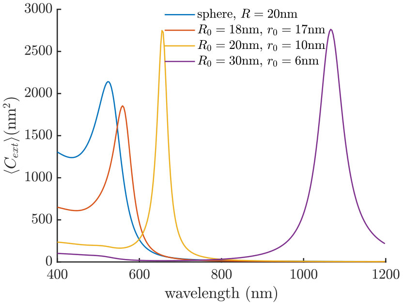 Figure 1
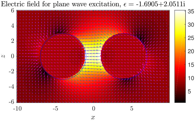 Figure 2
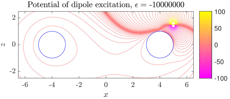 Figure 3
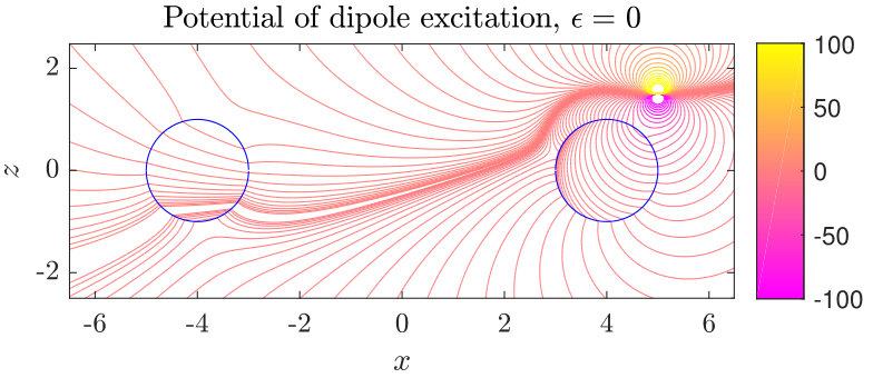 Figure 4
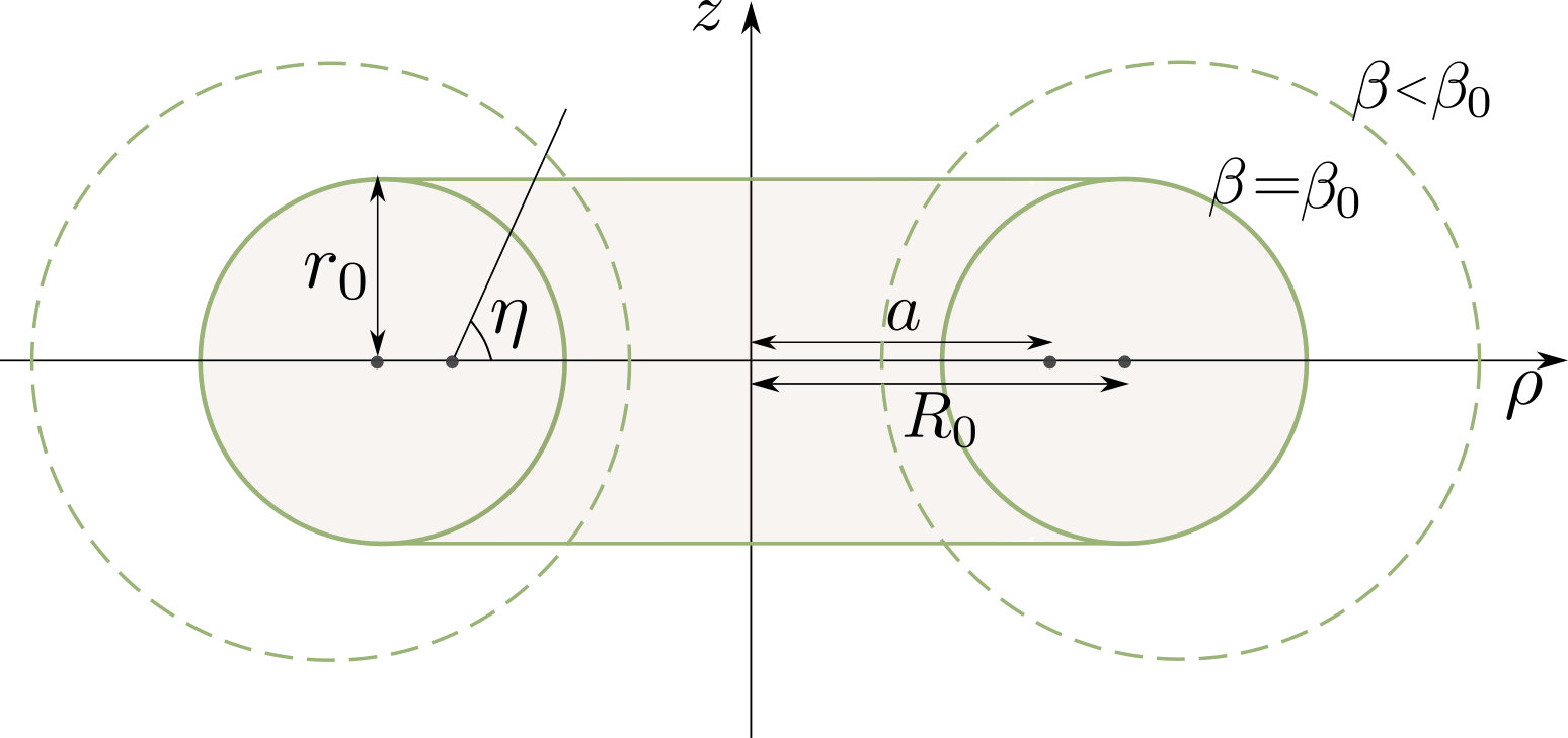 Figure 5
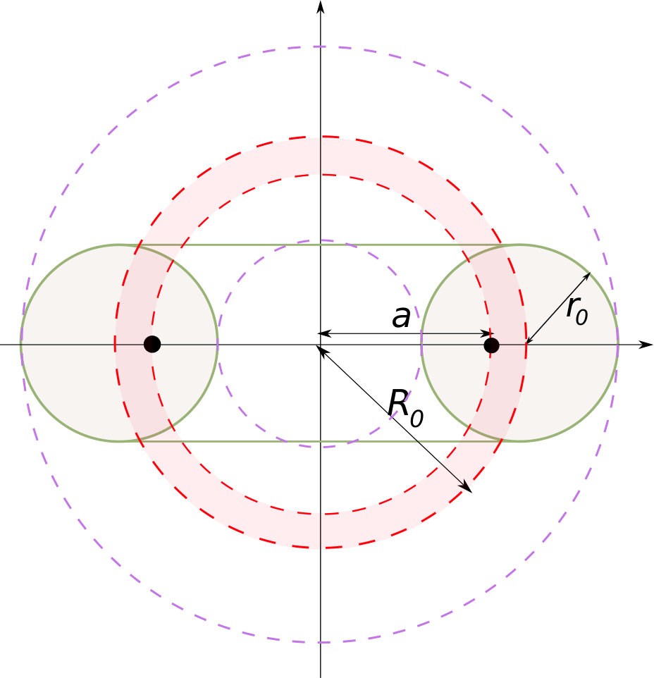 Figure 6
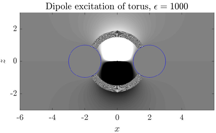 Figure 7
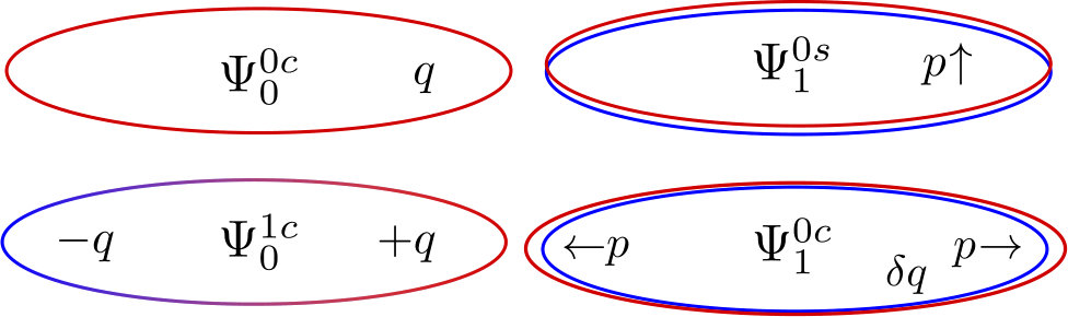 Figure 8
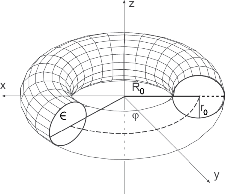 Figure 9
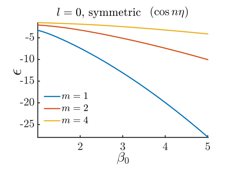 Figure 10
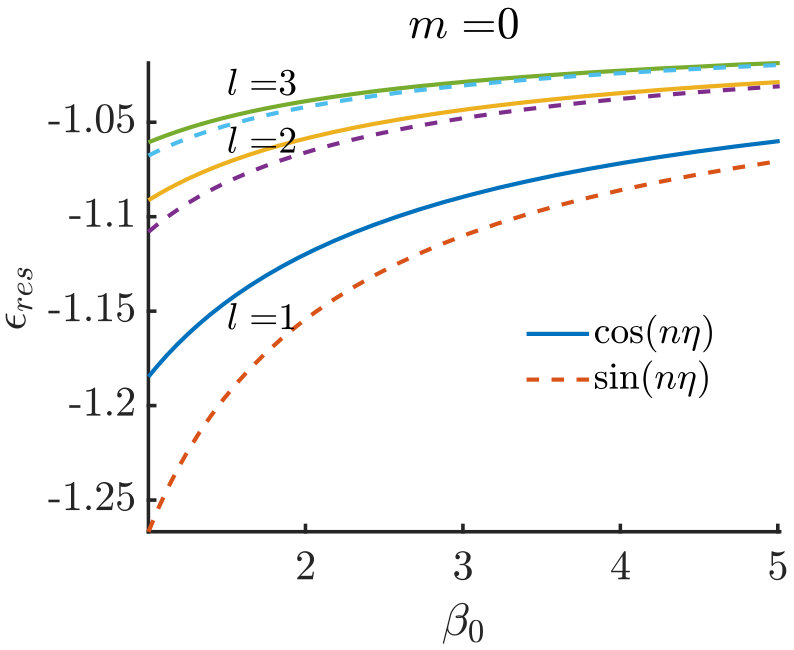 Figure 11
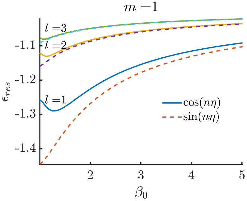 Figure 12
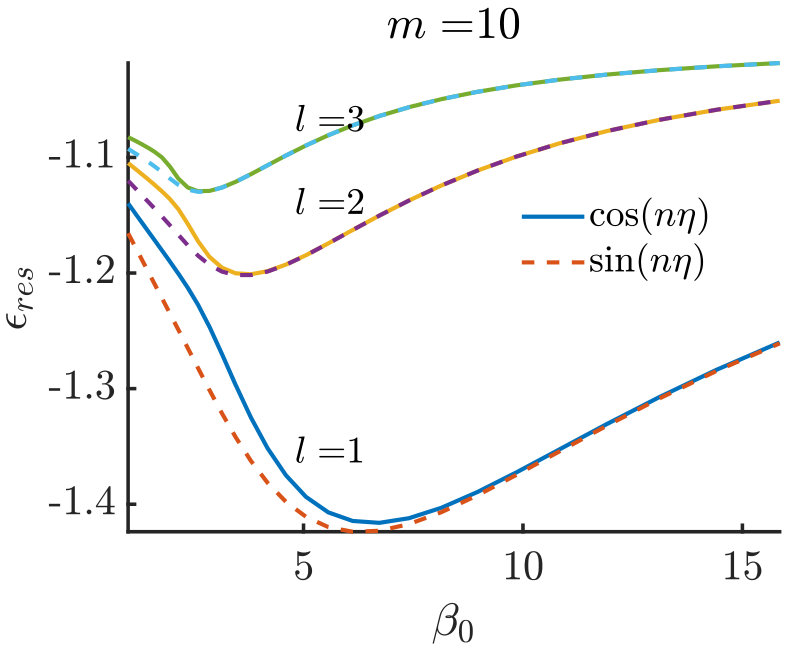 Figure 13
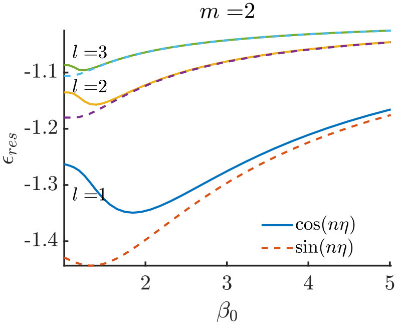 Figure 14
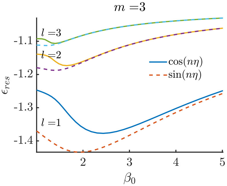 Figure 15
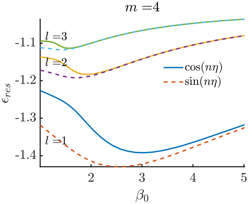 Figure 16
Peer Reviews
No public reviews on file for this paper yet. If you reviewed it on a platform where reviews are public (OpenReview, ICLR, NeurIPS, ICML), you can paste yours below so the community can read it here.
Videos
No videos yet. Explain this paper in a talk, walkthrough, or lecture? Add one.
Electrostatic -matrix for a torus on bases of toroidal and spherical harmonics
Matt Majic
The MacDiarmid Institute for Advanced Materials and Nanotechnology, School of Chemical and Physical Sciences,
Victoria University of Wellington, PO Box 600, Wellington 6140, New Zealand
Abstract
Semi-analytic expressions for the static limit of the -matrix for electromagnetic scattering are derived for a circular torus, expressed in bases of both toroidal and spherical harmonics. The scattering problem for an arbitrary static excitation is solved using toroidal harmonics and the extended boundary condition method to obtain analytic expressions for auxiliary and -matrices, from which the -matrix is given by their division. By applying the basis transformations between toroidal and spherical harmonics, the quasi-static limit of the -matrix block for electric multipole coupling is obtained. For the toroidal geometry there are two similar -matrices on a spherical basis, for computing the scattered field both near the origin and in the far field. Static limits of the optical cross-sections are computed, and analytic expressions for the limit of a thin ring are derived.
I Introduction
The -matrix method is a semi-analytical tool for calculating the properties of electromagnetic or acoustic scattering by macroscopic particles Waterman (1965); Mishchenko et al. (2002). The incident and scattered electromagnetic fields are expanded on bases of orthogonal functions, e.g. spherical wavefunctions, and the -matrix essentially outputs the series coefficients of the scattered field in terms of the known coefficients for the incident field. The -matrix may be calculated via the extended boundary condition method (EBCM) which involves numerically evaluating surface integrals, however this approach is unstable for particles with highly non-spherical shape, and much work has been done on determining conditions for the -matrix to be applicable Farafonov et al. (2016); Kyurkchan et al. (1996). For the EBCM to work, the Rayleigh hypothesis is historically suggested as criteria, which is the assumption that the series of basis functions converge on the entire surface of the particle, although it is known that this is not necessary and weaker criteria have been suggested Farafonov et al. (2016). The EBCM fails for certain convex particles, let alone multiply connected particles such as a torus.
Using other methods, scattering by a torus has been considered analytically in the long wavelength limit using toroidal harmonics, the partially separable solutions to Laplace’s equation in toroidal coordinates. Toroidal harmonics are a relatively new tool in computational physics due to their complexity. Also, being only partially separable solutions makes toroidal harmonics difficult to apply to problems even involving the torus. For conducting tori, fairly simple series solutions can be obtained in the static limit, but for dielectric tori, the series coefficients are not explicit. The coefficients are calculated using a three step recurrence relation, with initial values given by a continued fraction. Here we use an alternative approach to this recurrence scheme by computing the -matrix on a basis of toroidal harmonics. The series coefficients are then given by a matrix inversion. Some specific simulations include a dielectric torus in a uniform field Love (1972), a conducting torus illuminated by a low frequency plane wave Venkov (2007), plasmon resonances Dutta et al. (2008) and electromagnetic trapping Salhi et al. (2015). A detailed computational analysis of quasistatic scattering by solid and layered tori is conducted in Garapati et al. (2017). Semi analytical results for low frequency dipole excitation of simple geometries - a conducting torus Vafeas (2016), spheroids Vafeas et al. (2009) and two spheres Vafeas et al. (2012) are obtained for the lowest three orders in frequency of the electric and magnetic fields. The problems were formulated using the natural harmonic functions for the geometry, but it is also practical and insightful to recast these solutions in terms of spherical harmonics.
Spherical harmonics are far easier to compute, better known and more applicable than toroidal harmonics, so it is of interest to re-express this -matrix on a basis of spherical harmonics - in particular, this allows computation of the long wavelength limit of the -matrix for electromagnetic or acoustic scattering, which is usually expressed on a basis of spherical wavefunctions. For the spheroid, the low frequency scattering problem has been re-expressed with spherical harmonics and the electromagnetic -matrix has been obtained to third order in size parameter Majić et al. (2017); Majić and Le Ru (2019); Majic et al. (2019) by applying the series relationships between spherical and spheroidal harmonics. But the series relationships between spherical and toroidal harmonics are more complex and virtually unknown in the literature, exept for the low degrees: toroidal harmonics of degree zero, corresponding to the potential of rings of sinusoidal charge distributions, are known as series of spherical harmonics, and spherical harmonics corresponding to point charges and dipoles are known as series of toroidal harmonics. The relationships for all degrees and orders have been derived in a Russian paper from 1983 Erofeenko (1983), although this does not appear to be well known except for one other paper Shushkevich (1998), which analysed the electrostatic interaction between a conducting torus and a partial spherical shell - they used the relationships to construct what is effectively the -matrix for the conducting torus (eq. (32)), expressed on a spherical basis, as part of the kernel of an integral equation.
Contents
- •
Section II:
toroidal coordinates and harmonics are defined along with the charge distributions which generate these harmonics.
- •
Section III:
the scattering problem for a torus is formulated where the incident field is assumed to be expanded as a series of toroidal harmonics, and using the electrostatic null field equations, a toroidal -matrix is derived which gives the scattered field also on a basis of toroidal harmonics.
- •
Section IV:
Relationships between spherical harmonics are presented, with a new simple recurrence for their expansion coefficients.
- •
Section V:
these relationships are used to re-expresses the -matrix on a spherical harmonic basis.
- •
Section VI: plots of the potential and electric field, and presents physical quantities including capacitance, polarizability, plasmon resonances and optical cross-sections.
- •
Section VII:
Analytic asymptotic expressions for the -matrix elements in the thin ring limit.
- •
Appendix:
Derivations of the expansions between spherical and toroidal harmonics along with some interesting recurrence relations, explicit forms, a generating function and symmetries of the expansion coefficients, aswell as symmetries between spherical and toroidal harmonics.
II Toroidal coordinates and harmonics
Firstly we introduce spherical coordinates , and cylindrical coordinates . The toroidal coordinate system also uses a parameter which defines the radius of the ”focal ring” centred at the origin. Toroidal coordinates are then defined as
[TABLE]
with . corresponds to the torus size ( is a tight torus covering all space and is the focal ring) and relates to the angle around the minor axis.
Laplace’s equation is partially separable in toroidal coordinates, so that the solutions have an additional prefactor. The toroidal harmonics are defined for integer as
[TABLE]
where and are the Legendre functions of the first and second kinds. Using the superscript to denote or , we will call the “ring toroidal harmonics” and the “axial toroidal harmonics” since they are singular on the focal ring and -axis respectively. There are two kinds of angular solutions - which are symmetric about the meridian plane and which are antisymmetric. Compare this to spherical harmonics which have angular solutions and where the second type of angular solutions are discarded due to their singularity at the poles of the sphere. Toroidal harmonics also are non-zero for - as shown in the next section, this occurs (with for example) for a single ring with charge distribution . So all and for integer and are physically applicable solutions - smooth on the torus surface. And toroidal harmonics of negative or may be defined simply through
[TABLE]
II.1 Charge distributions of ring toroidal harmonics
In order to give insight, we investigate the charge distributions that create toroidal harmonics. are finite everywhere except , on the focal ring. We want to express the functions as integrals of charge distributions on this focal ring, weighted by the inverse distance between a point on the focal ring and an observation point . We start with , looking at (note that ). The Legendre functions approaching the ring behave as
[TABLE]
while . Approaching the focal ring, becomes equal to the distance from the ring. Compare this to approaching infinitely close to a line source with arbitrary charge distribution, where the potential goes as if the charge has unit density at the point of closest approach. The distance in cylindrical coordinates is . And the charge distribution must be proportional to , so we deduce that
[TABLE]
We should also check the limit as . Here , , and , so we can rule out the possibility of sources at .
The harmonics for may be generated by application of the operators and (see appendix B.1 for details), so we apply these to the integral expression (14), first :
[TABLE]
The charge distribution is two oppositely charged rings on the -plane, one with an infinitesimally greater radius than the other. This produces an infinitesimal charge imbalance - a net monopole moment, which is seen in the spherical-toroidal expansions (53).
And for :
[TABLE]
This is the potential of two oppositely charged rings with an infinitesimal separation in the -direction. These charge distributions are represented in figure 1.
For higher the harmonics can be generated by repeated application of the operator . We leave the details for appendix B.1, but state that the toroidal harmonics follow a recurrence relation (115) involving , and this recurrence is also satisfied by coefficients , relating toroidal and spherical harmonics (see (57)). We can then deduce the differential operators that generate the order harmonic from the or order harmonics:
[TABLE]
where is equal to with and similarly for . (18) starts from because . Both and are degree polynomials in .
The corresponding integral expressions for are given in operator form by applying (17) and (18) to the integral expression for (14) and (16). However, explicit evaluations of these derivatives do not appear to reveal any simple patterns. The integral expressions for have been checked numerically up to .
II.2 Charge distributions of axial toroidal harmonics
We will use heuristic arguments to derive the line source distributions for , which are singular on the axis. First consider . As in the previous section, we use the fact that for an arbitrary line charge distribution, close enough to the line, the potential will only depend on the magnitude of the charge distribution at the point of approach. So we can determine the line charge distribution by matching it to the limit of the potential as it approaches the line. The exact proportionality is obtained by considering that the potential near a line source with unit magnitude goes as . The behaviour of the components of the toroidal harmonics as are, using :
[TABLE]
Then the line source distribution of must be (using complex notation to deal with and simultaneously):
[TABLE]
And for , we have and there is no contribution from sources at . This is unlike the spherical harmonics of the second kind , whose charge distributions are the difference between a line source that produces an infinite potential and a sum of multipoles at infinity of infinite strength (work currently in progress).
Note that function makes the charge distribution continuous, and that it can also be expressed in terms of Chebyshev polynomials of the first and second kinds and :
[TABLE]
For , the charge distributions are multi-line, which can be deduced from the dependence. For example has a charge distribution of two line sources infinitely close together but of opposite charge. The behaviour of the Legendre functions is:
[TABLE]
So for we have, as .
And in the limit , we have . Despite the divergence for , there is no contribution from sources at , which can be explained as follows. If sources at existed, then we can split into its contributions from charges on the -axis and at . The potential due to charges at , being finite at the origin, can then be expressed as a series of regular spherical harmonics of the same as . However, where , so it is impossible to express the dependence as a series of . Therefore there cannot exist charges at .
We can compare to the potential near an -fold line charge distribution which similarly goes as as , with integral kernel . (25) for also shows a non-constant -dependence . Putting this together gives
[TABLE]
Andrews (Andrews (2006)- eq. 27) proved (26) via direct integration for all , and (in his notation ).
III -matrix for a torus on a toroidal harmonic basis
Consider a circular torus with major radius , minor radius and relative permittivity to the surroundings as shown in figure 2. The surface is defined by the aspect ratio , and the focal ring radius is . The torus is excited by an arbitrary external electric potential , and we want to determine the scattered potential (where ), and internal potential . The boundary conditions are:
[TABLE]
The fields are assumed to be expanded in terms of toroidal harmonics as
[TABLE]
In this section we derive the matrix relations between the incident, scattered, and internal expansion coefficients.
In general the boundary conditions are difficult to solve, and may lead to an inhomogeneous three term recurrence relation with initial conditions given by an infinite continued fraction Love (1972). Instead we will use the boundary integral equation formulation to find an analogue of the -matrix in toroidal coordinates. The boundary integral equations are derived from Green’s second identity on the torus surface Farafonov (2014):
[TABLE]
where is the derivative with respect to the surface normal and is the infinitesimal surface element. In the -matrix approach, Green’s function is expanded as a series of separable harmonics; here we use toroidal harmonics:
[TABLE]
We now substitute (32) and the expansions of the potentials into the integral equation(31), and equate the coefficients of the toroidal harmonics. For example, equating the coefficients of for inside the torus leads to (dropping the integration primes):
[TABLE]
The sum over has been omitted because the torus is rotationally symmetric and only terms with the same in the expansions of the and survive the integration. This decouples the problem for each . Furthermore, the integration is over an even interval of so integrates to zero, decoupling the sine and cosine expansion coefficients. The relationships between the expansion coefficients can be formulated with infinite dimensional matrices. For each , the problem is solved by the following matrix relations:
[TABLE]
which are analogous to the P, Q, -matrices in the -matrix method for scattering of waves. are ( being the numerical truncation order) column vectors containing the elements for fixed . When convenient the superscripts and will be omitted.
For a conducting torus, and the -matrix is diagonal:
[TABLE]
which is equivalent to well known solutions for conducting tori, see for example Scharstein and Wilson (2005).
For general , the integral equations 31 allow us to calculate and , while is obtained from
[TABLE]
We now look for analytic expressions for the matrix elements. In toroidal coordinates the normal derivative and surface element are
[TABLE]
Putting these into (33) and simplifying leads to an integral expression for :
[TABLE]
The first integral is simple:
[TABLE]
and the second integral evaluates to
[TABLE]
See appendix A for proof. For the integrals are
[TABLE]
and
[TABLE]
The matrix elements are then
[TABLE]
A similar derivation shows that is related to by
[TABLE]
for all . Hence the -matrix can also be expressed as
[TABLE]
We suspect this form applies to the -matrix for any particle who’s geometry is a coordinate of a coordinate system with partially-separable solutions to Laplace’s equation, including bispherical coordinates (in preparation). may be calculated via (36) or (46); both give the same numerical accuracy. To avoid possible numerical instability in inverting , the matrix should be transposed, inverted then transposed back.
The static limit -matrix for any scatterer is symmetric when expressed on a basis of normalised spherical harmonics or wave functions. This is proved in Farafonov and Ustimov (2015) by equating solutions from two surface integral equations similar to (31), given in Farafonov (2014). The proof used a basis of normalised spherical harmonics but could be easily done with any orthonormal basis. The basis functions are orthogonal but not normalised - they have a norm of . Hence the toroidal -matrix has the following symmetry property:
[TABLE]
III.1 Comparison to recurrence approach
Another way to solve electrostatic problems for the dielectric torus is to apply the boundary conditions in differential form (27) directly to the series expansions for the potentials (28-30), to obtain a recurrence relation for the coefficients. This has been done for a uniform electric field Love (1972), and point charge Kuyucak et al. (1998). For arbitrary excitation, we get
[TABLE]
The difficulty in computing the coefficients using this scheme is finding the initial values; these are expressed as a series of products of continued fractions. Nevertheless, we can compare this to the -matrix approach. Combining recurrence (48) with the definition of the -matrix, (34), we find
[TABLE]
which must hold for any set of coefficients . In particular if we choose an excitation with for some , a recurrence for the elements of the toroidal -matrix can be found:
[TABLE]
Which has been used as a check for the -matrix.
IV Relationships between spherical and toroidal harmonics
In order to express the -matrix on a basis of spherical harmonics, series relationships between spherical and toroidal harmonics are needed. We define the regular and irregular solid spherical harmonics as:
[TABLE]
In the appendix we derive the following linear relationships between spherical and toroidal harmonics:
[TABLE]
are rational numbers with many equivalent explicit forms and recurrence relations (see appendix B.3). For now they may defined by the stable recurrence:
[TABLE]
and the same for . The initial values are
[TABLE]
(the double factorial can be extended to odd negative integers via recurrence, or equivalently through the gamma function). Note for :
[TABLE]
The Legendre functions at 0 are, for :
[TABLE]
IV.1 Existence of expansions
Toroidal harmonics do not follow the same notion of internal and external as spherical and spheroidal harmonics. Ring harmonics can be written as a series of either internal or external spherical harmonics, due to the fact that they are finite at both the origin and at . However the axial toroidal harmonics are singular at the origin and infinity, so cannot be expanded as a series of spherical harmonics at all 111They can neither be expressed as a series of spherical harmonics of the second kind, or which are also singular on the axis. This is due to differences in parity about . Also, neither internal and external spherical harmonics can be expressed as a series of ring harmonics . This is because a series of ring harmonics can only converge outside some toroidal boundary, and this boundary must enclose the singularities of the function being expanded - the external spherical harmonics are singular at the origin, so this toroidal boundary must cover the origin and thus extend to all space, while the internal spherical harmonics cannot be expanded for a similar reason - the torus must extend to all space to cover the “singularity” at . Contrarily, both internal and external spherical harmonics can be expanded with axial toroidal harmonics , because a series of axial toroidal harmonics will converge inside some torus - for the internal spherical harmonics, this toroidal boundary may extend up to infinity since the functions are continuous in all space. For external spherical harmonics the toroidal boundary may extend to the origin. To check this we can determine the boundary of convergence of expansions (55) and (56) from the behaviour of the term in the series as . The Legendre functions grow as DLMF pg 191 ((61) is presented for completeness):
[TABLE]
while and are bounded by the sequence (with the same initial values), which itself grows slower than . So the series coefficients decay geometrically as , and everywhere except the -axis and , so the series converge everywhere, although slowly near the axis and for large . In these cases the series terms grow significantly in magnitude before converging, which sacrifices accuracy because the series can only be accurate to the last digit of the largest term in the series. This causes problems in dealing with extremely tight tori.
V -matrix on a spherical harmonic basis
For any bounded scatterer, the scattered field is expandable on a basis of outgoing spherical harmonics that converge outside the circumscribing sphere, and by linearity of Laplace’s equation, the expansion coefficients are linearly related to the coefficients of the incident field. Therefore the -matrix for any bounded scatterer should exist on a basis of spherical harmonics. In fact for a torus, the incident and scattered fields may both be expanded on interior or exterior spherical harmonics (see sec. V.1). First we look at the standard case where the external field is expanded on regular spherical harmonics and the scattered field will be expanded on irregular harmonics. So the potentials are assumed to have the following expansions:
[TABLE]
the sum over can be written in matrix notation so that
[TABLE]
where for example , are ( being the numerical truncation order) column vectors containing the elements or for all , for a fixed , and is the -matrix. The vectors and matrices start their index from even though the spherical harmonics are zero for ; this is match the dimensionality of the toroidal matrices which start from .
It is most likely not possible to expand the internal potential as a series of spherical harmonics, following the logic of section IV.1. We know may be represented as a series of toroidal harmonics which are singular on the -axis, so it is a fair assumption that the analytic continuation of is singular on atleast the -axis (although not proven - it may be possible that a series of functions that are singular in some region could cancel exactly resulting in a smooth function, but given the complex series coefficients, this seems unlikely). This singularity would prohibit expansions in terms of both external or internal spherical harmonics since every spherical annulus would contain singular points. This means that the and matrices have no representation on a spherical basis, and therefore it would be impossible to compute the -matrix directly via the extended boundary method on a spherical basis. However, since the problem can be solved using toroidal harmonics, we can use this and apply the spherical-toroidal transformations of section IV without considering .
For this it will be useful to express the relationships between spherical and toroidal harmonics in matrix notation:
[TABLE]
where the elements of matrices and can be determined from (53,54,55) to be
[TABLE]
The subscripts stand for regular or irregular (referring to the type of spherical harmonic), and the superscripts refer to cosine or sine of .
First the excitation potential in (65) must be expressed on a basis of toroidal harmonics by applying (67):
[TABLE]
then is found via the toroidal-basis -matrix solution (34):
[TABLE]
and expanding the toroidal functions back into spherical harmonics with (68):
[TABLE]
Comparing this to (66), and noting that , the -matrix is found to be
[TABLE]
The term contributes to the entries of with only and both even, while contributes only to entries with and both odd. Hence for odd as expected for particles with reflection symmetry about .
Here we have not used normalised spherical basis functions, and as a consequence is not symmetric for . The quasistatic limit of the conventional symmetric electromagnetic -matrix in Mishchenko et al. (2002) can be obtained from:
[TABLE]
where is the wavenumber in the surrounding medium.
V.1 Interior/exterior -matrices
In the above derivation we assumed that the external potential was created by a source that could be expanded as a series of regular spherical harmonics, but because the torus excludes the origin, the external field may come from near the origin (for example a point source at the origin) and irregular harmonics must be used instead. Similarly, to compute the scattered field near the origin, a regular basis must be used. The -matrix derived above applies only if is expanded on and is expanded on , and we denote this matrix . Following similar derivations, expressions for the other matrices can be found, and all four variations of these -matrices are
[TABLE]
The transformation matrices not already defined in (69) differ only in alternating signs, and are
[TABLE]
For example, applies if the source is outside the torus’ circumscribing sphere, and if the scattered field is to be evaluated near the hole.
For a conducting torus two pairs of these -matrices in (75) are identical. Mathematically it is straightforward to show that . Physically this is due to the fact that the problem for a conductor does not distinguish the scattered and external/incident fields - the problem of determining the incident field from the scattered is the same as determining the scattered from the incident. And , which can be shown by applying radial inversion about the sphere of radius centred at the origin. The geometry transforms as which preserves the torus, while potentials transform as , so . This argument only applies to the conducting torus since permittivity also transforms as .
From the static -matrix we can make deductions of the applicability of the full-wave -matrix. Since the high order limit of the spherical wave functions tends towards the solid spherical harmonics, the boundaries of convergence of the full wave solution are identical to that for the quasistatic solution. It is not possible to compute the scattered field in a spherical annulus around the mid section of the torus , due to the singularity of the scattered field. Even in the case of a charged conducting torus (constant external potential), it can be shown that both the interior and exterior spherical harmonic solutions diverge in the annulus . This is analogous to spheroids with high aspect ratio - there is a region near the spheroid where the fields cannot be expressed using spherical basis functions.
VI Derived physical quantities
We now use these methods to calculate spatial fields, capacitance, polarizability, resonance conditions and cross sections.
VI.1 Spatial fields
To verify the boundary conditions for the potential we look at the extreme cases of a conducting () and extremely non-conducting torus () in figure 3. In both cases the equipotentials visually satisfy the boundary conditions in (27). For a conducting torus the results for coincide with conducting solution (35).
Since gold nanoparticles are often used for their field enhancements, the electric field is plotted for a gold nano-torus in water excited by a uniform field, showing a strong field enhancement in the gap. The plots in figures 3, 4 have also been calculated using the spherical -matrix and spherical harmonics, to verify that both approaches converge to the same result (atleast where the spherical solution converges).
VI.2 Capacitance and dipolar response of conducting torus
The capacity of a conducting torus held at a uniform potential can be deduced from the induced charge , and is related to :
[TABLE]
And for the dipole polarizability we consider a uniform field along a cartesian axis, exciting dipole moment in a conducting torus. The polarizability is related to :
[TABLE]
where
[TABLE]
These results agree with Belevitch and Boersma (1983).
VI.3 Plasmon resonances
From the explicit expressions for the toroidal matrices in (43,44), we can calculate the values of that produce - a plasmon resonance. These are for , , . We have replaced the index with because each resonant mode consists of all toroidal harmonics for , not accentuating one in particular. A natural choice is to let order these in terms of magnitude ( are all negative real numbers), which appears to also order the resonances in terms of strength. can be found from the condition , through where are the eigenvalues of and . Note that is independent of .
In figure 5 the conditions for resonances are plotted as a function of aspect ratio , and agree with the continued fraction approach Avramov et al. (1993); Love (1975); Garapati et al. (2017). Also, these results confirm the discussion of Salhi (2016) claiming that resonances exist, even though they were not obtained in Love (1975); Avramov et al. (1993).
VI.4 Optical cross sections
The cross sections are obtained from the elements of the full-wave -matrix Mishchenko et al. (2002). In the small particle limit, only the dominant terms for contribute. For example we look at the orientation averaged cross-sections:
[TABLE]
with
[TABLE]
The extinction cross-section is plotted in figure 6 for various nano-tori and appear consistent with results from El-Shenawee et al. (2009); Salhi et al. (2015); Mary et al. (2007). The dominant response comes from - excitation along the - plane - this is the plasmon resonance in figure 5. We cannot see the resonances for that occur for small negative epsilon due to the considerable imaginary part of the dielectric function of gold. On the other hand, is almost negligible and has no resonance.
VII Thin ring limit
We can find analytic results for the matrix elements in the thin ring limit. The limits of the Legendre functions are DLMF
[TABLE]
and we will need to second order:
[TABLE]
which can be obtained from its hypergeometric function definition. (88) agrees with Scharstein and Wilson (2005) as for , but is more accurate. It can be shown that the toroidal -matrices in this limit are lower triangular - for , with
[TABLE]
Now we use the -matrix , which has the following limit:
[TABLE]
This expression for is the inverse of in (92), i.e. , which can be proven with the help of Mathematica. To obtain a result for the -matrix entry , it is also necessary to include the second order for the element :
[TABLE]
The second order for is obtained by including the 2nd order element (above the diagonal) and inverting the matrix consisting of just the top left block of . Then the -matrix (95) is obtained through (46):
[TABLE]
The upper diagonal entries of with can be obtained from the symmetry property of the toroidal -matrix (47). In this limit there is just one resonance at , consistent with the trends seen in figure 5 for large , and the resonance for a cylinder. All elements have been checked numerically against the exact matrix elements in section III.
An important feature is that the top left 22 square of are all order , while all other entries decay quickly as , meaning that modes for dominate both the excitation () and response (). For , there is only one dominant element, .
We can now determine limits for the static dipolar polarizabilities per unit volume, to , using (86,87) with (95):
[TABLE]
These produce reasonable accuracy () for aspect ratios , but fail when . It is interesting to compare these to the polarizabilities of a thin prolate spheroid, or needle:
[TABLE]
, apply when the long dimension of the wire is perpendicular to the applied electric field, and in fact both are of the form . On the other hand and both diverge as , where the long dimension of the wire is aligned with the electric field. is of the form . Intuitively, for the ring is half aligned perpendicular and half parallel to the incident field, so that .
Numerical tests show that for very large —— and very thin rings, the approximate expressions for break down, particularly for . For analysis of the thin ring limit for conducting tori, see Scharstein and Wilson (2005).
VIII Conclusion
The problem of a dielectric torus in an arbitrary electrostatic field has been solved semi-analytically, and expressions are found for the -matrix on both a toroidal and spherical harmonic basis. New forms of the series relationships between spherical and toroidal harmonics were derived. Resonant permittivities are calculated from matrix eigenvalues and agree with results from solving a continued fraction equation. Fully analytic asymptotic expressions are given in both the conducting and thin ring limits. The -matrix has been linked the time-harmonic -matrix governing electric multipole interactions, . These results prove the existence of the -matrix for such a complex shape, atleast in the small size limit. It is also found that similar -matrices can be defined depending on whether the source is near or far from the torus hole and whether the scattered field is to be evaluated near or far from the origin.
Hopefully this approach of applying basis transformations to the spherical harmonics and evaluating the surface integrals can be used to numerically obtain the -matrix for other objects with ring like geometry.
To extend these results to the Helmholtz equation, we would need a basis suited to the toroidal geometry but unfortunately the Helmholtz equation is not separable in toroidal coordinates. A basis of toroidal wavefunctions were presented in Weston (1960), although these are not orthogonal.
A similar work is in preparation on bispherical coordinates and scattering by two spheres. Bispherical and toroidal coordinates essentially differ by a real/imaginary focal distance, and the corresponding harmonics differ by a shift of the separation constant by , however, the topology of the two systems is radically different.
Acknowledgements.
I wish to thank my supervisor Eric C. Le Ru for helpful discussions, and Victoria University of Wellington for financial support through a Victoria Doctoral Scholarship.
Appendix A Evaluation of the surface integral (40)
First we express the integral using the product formula:
[TABLE]
Following the method of Mason and Handscomb (2002) (lemma 8.3) with minor changes we make the substitutions , , and rewrite the first integral as
[TABLE]
There are two poles inside the integration path, a simple pole at and a pole of order at . Applying the residue theorem we find:
[TABLE]
Then combine this with (100) to obtain (40). The proof of (42) is similar.
Appendix B Derivations of the relationships between spherical and toroidal harmonics
B.1 Expansions of toroidal harmonics
We can first obtain the expansions of toroidal harmonics in terms of spherical harmonics , by equating two expansions of Green’s function. For points and with , the spherical harmonic expansion of Green’s function is Morse and Feshbach (1953)
[TABLE]
In this document are defined without the phase , while .
Also we have the ’cylindrical’ expansion Cohl and Tohline (1999):
[TABLE]
which converges in all space except at . Note .
Evaluating both (103) and (104) at (, , ), and equating the term gives for :
[TABLE]
Similarly the expansion for can be found by setting in (103) and (104):
[TABLE]
The left hand side is actually proportional to the toroidal harmonic . This can be seen by application of the Whipple formulae, which expressed in toroidal coordinates read as
[TABLE]
We may then rewrite the expansions (105,106) as
[TABLE]
which is (53) for . (109) has been generalized to the Helmholtz equation (harmonic time dependence), as a spherical wave function expansion of a circular ring with current distribution expressed as a Fourier series Hamed (2014).
The toroidal harmonics are the potential of a ring of dipoles pointing in the -direction. This can be obtained by applying the operator which transforms a charged ring into a double ring with dipole moment in the -direction. Explicitly:
[TABLE]
is also a ladder operator for the spherical harmonics:
[TABLE]
Applying to the toroidal harmonic expansion (109), and noting an identity for the derivative of the Legendre functions, leads directly to the expansion for .
is the potential of a ring of dipoles oriented outwards from the origin. To generate this we apply which preserves harmonicity as does , but turns a ring of charge on the plane into a ring of dipoles pointing inward, plus, as it turns out, a net charge on the ring, as noted in section II.1.
Applying to the toroidal harmonic expansion (109) and rearranging gives the expansion for . We can now derive the expansions for general by repeated application of . For the spherical harmonics:
[TABLE]
applying to and rearranging, making use of the product to sum formulae for trigonometric functions and the recurrence relation for the Legendre functions for increasing , we obtain:
[TABLE]
By assuming some expansion coefficients , for the expansions of the toroidal harmonics as in (53,54), we can deduce that they satisfy the recurrence relation (57), which is sufficient to calculate the coefficients for all without numerical problems.
The first few orders for are:
[TABLE]
Although these coefficients may be computed for all integer , are only relevant for even, while only for odd.
B.2 Expansions of spherical harmonics
We start by applying a trigonometric identity to rearrange the toroidal Green’s function expansion Morse and Feshbach (1953) as
[TABLE]
and substitute the spherical harmonic expansions for point (53,54),
[TABLE]
and compare this to the spherical expansion of Green’s function (103), equating the coefficients of for all . This gives the expansion of spherical harmonics in terms of toroidal harmonics , as presented in (55,56).
Looking at the low orders, for , (55) is the expansion of a constant onto the basis of toroidal harmonics, and is known as Heine’s expansion. And for (56) is simply Green’s function expansion (116) for . And for , , (55) and (56) are expansions of uniform fields and point dipoles at the origin. Some low orders of the coefficients are
[TABLE]
B.3 Explicit forms of spherical-toroidal expansion coefficients
While the recurrence (57) is sufficient to accurately calculate the coefficients and , we here investigate more equivalent explicit forms and properties. First, Erofeenko Erofeenko (1983) deduced that these were related to the coefficients for expressing a product of trig functions as a series of powers of the tangent. Essentially they had
[TABLE]
where the notation means that rises in steps of 2. From this they derived explicit forms of the coefficients, and defined which dealt with and simultaneously:
[TABLE]
For , the identity for Legendre functions is implied. Also, in Erofeenko (1983) a dimensional factor of was included which we ignore here. was also found to have a triangular recurrence over and :
[TABLE]
which was obtained by application of instead of as in the derivation in section B.1. was actually generalised to consider the centre of the spherical coordinates being translated up the -axis - this is obtained essentially by replacing the 0 in with some angle. These generalised coefficients could be used to obtain the -matrix for the offset torus, allowing an analytic study of stacked tori, as considered in Salhi et al. (2015).
Also, by direct evaluation of the toroidal harmonic expansion (53) for on the -axis, using , we find:
[TABLE]
where are the Chebyshev polynomials. (123) can be seen to be equivalent to (119) by substituting and recognising that and .
We can also find the generating function. Adding (119) and (120) gives
[TABLE]
Substituting gives the generating function for :
[TABLE]
By expanding this via the binomial series for the numerator and denominator separately, and multiplying these, it is possible to find as a finite sum of binomial coefficients, then using an identity for the product of two binomial coefficients, we find
[TABLE]
which is equivalent to (121).
By application of eq. 7.12, vol. 4 of Gould (1990) to (126), we also obtain
[TABLE]
Using the generating function (125), it is possible to find two more recurrence relations:
[TABLE]
and a recurrence over only:
[TABLE]
(129) is similar in form to the recurrence over , (57), which for comparison we write here for :
[TABLE]
In fact if we define rational numbers which may be computed using (126), then is symmetric: . This symmetry is related to the fact that toroidal harmonics and spherical harmonics are of similar form, related by a symmetric coordinate transformation and index shift , as we will now show. Defining , , we have the following algebraic relationships between toroidal and spherical coordinates:
[TABLE]
The transformation between the coordinate systems is symmetric and can be expressed by the substitutions , . Also the separation constant can be modified by a factor so that its reciprocal is equal to itself under coordinate transformation:
[TABLE]
with these coordinates, we can rewrite the toroidal-spherical expansions in a very symmetrical form (for example just looking at expansions involving regular spherical harmonics , (53-55)):
[TABLE]
these are closely related by , , , . The main difference is that (130) is a series of while (131) involves , which is required for the series to converge since and .
Matlab codes are attached for computation of the Legendre functions, and the -matrix on both toroidal and spherical bases.
The reference list from the paper itself. Each links out to its DOI / PubMed record.
- 1Waterman (1965) P. Waterman, Proceedings of the IEEE 53 , 805 (1965).
- 2Mishchenko et al. (2002) M. I. Mishchenko, L. D. Travis, and A. A. Lacis, Scattering, absorption, and emission of light by small particles (Cambridge university press, 2002).
- 3Farafonov et al. (2016) V. Farafonov, V. Il’in, V. Ustimov, M. Prokopjeva, et al. , Journal of Quantitative Spectroscopy and Radiative Transfer 178 , 176 (2016).
- 4Kyurkchan et al. (1996) A. G. Kyurkchan, B. Y. Sternin, and V. E. Shatalov, Physics-Uspekhi 39 , 1221 (1996).
- 5Love (1972) J. Love, Journal of Mathematical Physics 13 , 1297 (1972).
- 6Venkov (2007) G. Venkov, Journal of Computational Acoustics 15 , 181 (2007).
- 7Dutta et al. (2008) C. M. Dutta, T. A. Ali, D. W. Brandl, T.-H. Park, and P. Nordlander, The Journal of chemical physics 129 , 084706 (2008).
- 8Salhi et al. (2015) M. Salhi, A. Passian, and G. Siopsis, Physical Review A 92 , 033416 (2015).