This paper introduces wave packet smoothness spaces, a new family of quasi-Banach spaces characterized by sparsity in frame expansions, and explores their structure, embeddings, and relations to classical function spaces.
Contribution
The paper defines wave packet smoothness spaces, constructs Banach frames and atomic decompositions, and analyzes their embeddings with classical function spaces.
Findings
01
Wave packet smoothness spaces include spaces characterized by sparsity in Gabor and wave atom expansions.
02
Banach frames and atomic decompositions are constructed for these spaces.
03
Embeddings between wave packet smoothness spaces and classical spaces like Besov and Sobolev are established.
Abstract
We introduce a family of quasi-Banach spaces - which we call wave packet smoothness spaces - that includes those function spaces which can be characterised by the sparsity of their expansions in Gabor frames, wave atoms, and many other frame constructions. We construct Banach frames for and atomic decompositions of the wave packet smoothness spaces and study their embeddings in each other and in a few more classical function spaces such as Besov and Sobolev spaces.
Ij:={i∈I:Qi∩Pj=∅} for j∈JandJi:={j∈J:Pj∩Qi=∅} for i∈I.
Ij:={i∈I:Qi∩Pj=∅} for j∈JandJi:={j∈J:Pj∩Qi=∅} for i∈I.
∃N∈N0∀i∈I∃ji∈J:Qi⊂PjiN∗;
∃N∈N0∀i∈I∃ji∈J:Qi⊂PjiN∗;
wi≤C⋅wℓfor all i,ℓ∈I and all j∈J for which Qi∩Pj=∅=Qℓ∩Pj;
wi≤C⋅wℓfor all i,ℓ∈I and all j∈J for which Qi∩Pj=∅=Qℓ∩Pj;
Peer Reviews
No public reviews on file for this paper yet. If you reviewed it on a platform where reviews are public (OpenReview, ICLR, NeurIPS, ICML), you can paste yours below so the community can read it here.
Videos
No videos yet. Explain this paper in a talk, walkthrough, or lecture? Add one.
Taxonomy
TopicsMathematical Analysis and Transform Methods · Image and Signal Denoising Methods · Advanced Harmonic Analysis Research
Full text
Design and properties of wave packet smoothness spaces
Dimitri Bytchenkoff 1,2,∗
Felix Voigtlaender 1,3,∗
1Technische Universität Berlin, Institut für Mathematik, Straße des 17. Juni 136, 10623 Berlin, Germany
2Université de Lorraine, Laboratoire d’Energétique et de Mécanique Théorique et Appliquée, 2 avenue de la Forêt de Haye, 54505 Vandoeuvre-lès-Nancy, France
3Katholische Universität Eichstätt–Ingolstadt, Lehrstuhl für wissenschaftliches Rechnen, Ostenstraße 26, 85072 Eichstätt, Germany
Abstract
We introduce a family of quasi-Banach spaces — which we call
wave packet smoothness spaces — that includes those function spaces which
can be characterised by the sparsity of their expansions in Gabor frames, wave atoms, and many other frame constructions.
We construct Banach frames for and atomic decompositions of the
wave packet smoothness spaces and study their embeddings in each other
and in a few more classical function spaces such as Besov and Sobolev spaces.
Résumé
Nous introduisons une famille d’espaces affines quasi-normés complets – que nous appellerons espaces de paquets d’ondelettes réguliers – qui incluent de nombreux espaces de fonctions caractérisés par leurs transformées, comme celle de Gabor ou en ondelettes, clairsemées. Nous construisons des cadres de Banach et des décompositions atomiques pour ces espaces et étudions leurs inclusions l’un dans l’autre ainsi que dans quelques espaces de fonctions devenus classiques tels que ceux de Sobolev ou de Besov.
A large number of different frame constructions are used in harmonic analysis
both in practical applications such as image denoising
[9, 45, 5, 53],
restoring truncated signals [51, 52],
edge detection [50, 41]
and compressed sensing [1]
and in pure mathematics for characterising
function spaces in terms of the frame coefficients
[44, 64, 27, 20, 58],
studying the boundedness of operators
[28, 47, 46, 37]
or for characterising the wave front set of distributions
[17, 39, 8].
The most important of these frame constructions are wavelets [14],
Gabor frames [27, 29],
shearlets [38, 40],
curvelets [7],
ridgelets [6, 30]
and wave atoms [15].
All of these frames are constructed by applying dilations, modulations and translations
to a finite set of prototype functions.
Since the seminal work of Cordoba and Fefferman [12] — who
used such systems to study the mapping properties of pseudo-differential operators — it has become
customary to refer to such systems as wave packet systems.
While the first papers mainly considered wave packet systems with continuous index sets
[12, 48], nowadays the focus lies on
discrete wave packet systems, which are special generalised shift invariant systems
[34, 43, 21, 59].
As particular highlights of the theory of wave packets, we mention the characterisation
of the Parseval property [35, 42]
for such systems and the use of Gaussian wave packets for approximating solutions
of the homogeneous wave equation [2].
In the present paper, we will concentrate on the case of functions on R2
and consider the class of (α,β) wave packet systems as introduced in
[15].
Here, the parameter α∈[0,1] describes the frequency bandwidth relationship
of the system, while β∈[0,1] describes its directional selectivity.
More precisely, if (ψi)i∈I is a system of (α,β) wave packets
and if ψi is concentrated at frequency ξ∈R2,
then the bandwidth of ψi is approximately (1+∣ξ∣)α.
The parameter α describes how multi-scale the system is.
For instance, for Gabor systems, the bandwidth of the
frame elements is independent of the frequency (α=0), while for
wavelets, the bandwidth is proportional to the frequency (α=1).
The parameter β determines how many different directions the
wave packet system can distinguish at each frequency scale; that is,
on the dyadic frequency ring {ξ∈R2:∣ξ∣≍2j},
an (α,β)-wave packet system distinguishes approximately
2(1−β)j different directions.
For instance, wavelets are directionally insensitive
(β=1), while Gabor frames have high directional sensitivity
(β=0).
Figure 1 shows how wave packet systems,
including their most important examples, relate to α and β.
Our contribution
In this work, we provide a rigorous mathematical framework for studying the
properties of (α,β) wave packet systems.
Specifically, for given 0≤β≤α≤1, we define
a family of wave packet smoothness spacesWsp,q(α,β), parametrised by the integrability
exponents p,q∈(0,∞] and the smoothness parameter s∈R,
and investigate properties of these spaces.
One of our main results is that if W(α,β)=(ψi)i∈I
is a sufficiently regular frame of (α,β)-wave packets, then
W(α,β) constitutes a Banach frame and an
atomic decomposition for a whole family of wave packet smoothness spaces.
We would like to emphasise that the wave packet system is not required
to be band-limited; on the contrary, we show that if the generators of the wave
packet system are compactly supported and smooth enough, then the
resulting wave packet system will constitute a Banach frame and an atomic
decomposition for a family of wave packet smoothness spaces provided that the
sampling density of the wave packet system is fine enough.
In a nutshell, this means that the wave packet smoothness space is
characterised by the decay of the frame coefficients with respect to the wave packet system.
More precisely, there is an explicitly given coefficient spaceCsp,q such that
[TABLE]
Moreover, a function f∈Wsp,q(α,β) can be
continuously reconstructed from its analysis coefficients(⟨f∣ψi⟩L2)i∈I, and the
synthesis coefficientsc(f)=(ci)i∈I∈Csp,q
satisfying f=∑i∈Iciψi can be chosen to depend
linearly and continuously on f.
In a less technical terminology, the
identity (1.1) means that
analysis and synthesis sparsity are equivalent for sufficiently
regular wave packet systems, where sparsity is quantified by the
coefficient space Csp,q.
We note that Csp,p=ℓp for a suitable choice of
s=s(p,α,β).
For non-tight frames, this equivalence between analysis- and synthesis sparsity
is nontrivial, but often useful.
For instance, it is usually relatively simple to verify that a certain class of
functions has sparse — or quickly decaying — analysis coefficients, which
amounts to estimating the inner products ⟨f∣ψi⟩L2.
In contrast, it can be quite difficult to construct coefficients
c=(ci)i∈I such that f=∑i∈Iciψi, even without
requiring that the sequence c has good decay properties.
For applications in approximation theory or for studying the boundedness
properties of operators, however, it is usually much more useful to know that
f=∑i∈Iciψi with sparse coefficients c,
rather than that the analysis coefficients of f are sparse.
The second of our main findings are several useful results
concerning embeddings of the wave packet smoothness spaces.
First, we study the existence of embeddings
[TABLE]
between wave packet spaces with different parameters.
Given (1.1),
this amounts to asking whether sparsity of a function f with
respect to an (α,β) wave packet system implies some, possibly worse,
sparsity with respect to an (α′,β′) wave packet system.
If β≤β′ and α≤α′ or if β′≤β
and α′≤α, we can completely characterise the
existence of the embedding (1.2).
Furthermore, we show that distinct parameter choices yield distinct wave packet smoothness spaces;
that is,
Ws1p1,q1(α,β)=Ws2p2,q2(α′,β′)
unless (p1,q1,s1,α,β)=(p2,q2,s2,α′,β′) or
(p1,q1)=(2,2)=(p2,q2) and s1=s2.
Finally, we also consider embeddings between wave packet smoothness spaces
on the one hand and Besov- or Sobolev spaces on the other hand.
For the case of Besov spaces, we again obtain a complete characterisation
of the existence of the embeddings
Ws1p1,q1(α,β)↪Bp2,q2s2(R2)
and of the reverse embedding; as a corollary, we show that
Bp,qs(R2)=Wsp,q(1,1).
For the case of Sobolev spaces, we can completely characterise
the existence of the embedding
Wsp,q(α,β)↪Wk,r(R2) for
r∈[1,2]∪{∞}.
For r∈(2,∞) we establish certain necessary and certain sufficient
conditions for the existence of the embedding, which are not equivalent.
In particular, we show that if s≥k+c(p), then
Wsp,q(α,β)↪Cbk(R2), so that
all functions in the wave packet smoothness space are k-times continuously differentiable.
This is one of the reasons for calling the spaces Wsp,qsmoothness spaces.
One can in principle define
wave packet systems for arbitrary α,β∈[0,1].
In this work, however, we restrict ourselves to the case where
0≤β≤α≤1 for defining the wave packet smoothness spaces
and to 0≤β≤α<1 for constructing Banach frames and atomic decompositions
for these spaces.
This restriction α<1 is mainly done for convenience,
since the case α=1 was already explored in [64],
which studies α-shearlet systems
and the associated smoothness spaces for α∈[0,1].
In our terminology, α-shearlets are (1,α) wave packets.
In contrast — at least with our construction of the wave packet smoothness spaces — the restriction
β≤α seems to be unavoidable.
Precisely, we define the wave packet spaces as decomposition spaces
[16] with respect to a certain covering of the frequency space,
which we call the (α,β) wave packet covering.
To show that this construction yields well-defined spaces, the wave packet covering
needs to satisfy a bounded overlap property; for this, the assumption β≤α
seems to be essential.
Finally, we are unaware of any frame construction that results in
(α,β) wave packets with β>α; as seen in
Figure 1, all commonly used
frame constructions fall into the regime β≤α.
Structure of the paper
To define the wave packet smoothness spaces
Wsp,q(α,β), we shall use the formalism of
decomposition spaces,
originally introduced in [16].
In order to define such a decomposition space
D(Q,Lp,ℓwq), one needs a coveringQ=(Qi)i∈I of the frequency domain
which has to satisfy certain regularity criteria;
namely, it has to be admissible and, preferably,
almost-structured.
In Section 2, we recall those parts of the existing
theory of decomposition spaces that are essential for our work.
In particular, we recapitulate the notions of admissible and almost-structured
coverings, the existing theory concerning the existence of embeddings between different
decomposition spaces, and the recent theory of structured Banach frame
decompositions of decomposition spaces.
In Section 3, we introduce the
wave packet coveringsQ(α,β) that we shall use
to define the wave packet smoothness spaces and verify that
Q(α,β) indeed covers the whole frequency plane.
That the covering Q(α,β) is admissible and almost-structured
is shown in Sections 4 and 5,
respectively.
The wave packet smoothness spaces will be defined in
Section 6, where we also study many of their
properties.
First, we show that they are indeed well-defined quasi-Banach spaces.
Second, we study the existence of embeddings
Ws1p1,q1(α,β)↪Ws2p2,q2(α′,β′)
between
wave packet smoothness spaces with different parameters
and show that distinct parameters yield distinct spaces.
Third, we will completely characterise the existence of embeddings
between inhomogeneous Besov spaces and wave packet smoothness spaces.
Fourth, we study the conditions under which the wave packet smoothness spaces
embed into the classical Sobolev spaces Wk,p(R2).
For the range p∈[1,2]∪{∞} we characterise these conditions
completely.
Finally, we show that the (α,α) wave packet smoothness spaces
are identical to α-modulation spaces.
Since our construction of the covering Q(α,β)
involves some non-canonical choice of parameters,
the spaces Wsp,q(α,β) might appear rather esoteric.
In Section 7, we show that this is not the case.
Precisely, we introduce the natural class of (α,β) coverings,
and show that any two (α,β) coverings give rise to the same family
of decomposition spaces. We also verify that Q(α,β)
is indeed an (α,β) covering.
This shows that the wave packet smoothness spaces are natural objects,
and it allows us to show that the wave packet smoothness spaces are invariant
under dilation with respect to arbitrary invertible matrices
(see Section 8).
Finally, in Section 9, we formally define the
notion of (α,β) wave packet systems.
We then show that the wave packet smoothness spaces can be described using
the decay of the analysis or synthesis coefficients with respect to
such a system. More formally, we show that if the generators of the
wave packet system are sufficiently smooth and decay fast enough,
then the associated wave packet system constitutes a Banach frame and an atomic
decomposition for a whole range of wave packet smoothness spaces provided
that the sampling density is fine enough.
The proofs of some particularly lengthy auxiliary statements were transferred
to Appendices A – C.
All general mathematical notions used in this manuscript
are summarised in Appendix D.
2 Decomposition spaces and their relation to frames and sparsity
Decomposition spaces, originally introduced by Feichtinger and Gröbner
[16], provide a unified generalisation of modulation
and Besov spaces and were used to introduce the α-modulation
spaces [25], which have recently received
great attention [36, 55, 32, 3, 19, 31, 33, 13].
The essential element of the decomposition space
D(Q,Lp,ℓwq) is the covering Q=(Qi)i∈I
of the frequency domain Rd. Given this covering, the Fourier transform
g of a given function g can be decomposed into the components
φi⋅g, where (φi)i∈I is a suitable
partition of unity subordinate to Q. The Fourier inverse
gi:=F−1(φi⋅g) of the components
φi⋅g are frequency-localised components
of the function g. The contribution of each of these components gi to the
decomposition space quasi-norm of g is measured by the Lp-norm, in the
time domain, and the total quasi-norm of g is obtained by using the weighted
ℓq space ℓwq as follows:
[TABLE]
To ensure that the decomposition space D(Q,Lp,ℓwq)
is indeed a well-defined quasi-Banach space, certain conditions must be imposed
on the covering Q, the partition of unity (φi)i∈I
and the weight w=(wi)i∈I.
These conditions and elementary properties of the decomposition spaces
D(Q,Lp,ℓwq) will be reminded in
Section 2.1.
An attractive feature of decomposition spaces is the recently developed theory
of structured Banach frame decompositions of decomposition spaces
[63], which shows that there is a
close connexion between the existence of a sparse expansion of a given function
f in terms of a given frame, and the membership of f in a certain
decomposition space, which depends on the frame under consideration.
This theory will be formally introduced in Section 2.2; here, we
outline the underlying intuition.
We first note that most frame constructions used in harmonic analysis
have two crucial properties:
•
The frame is a generalised shift-invariant system
(see [34, 59, 11, 21, 43] for more about these systems),
i.e., it is of the form Ψ=(Lxψj)j∈I,x∈Γj for
suitable generators (ψj)j∈I and certain lattices
Γj=δBjZd where the matrices Bj∈GL(Rd)
are determined by the frame construction
and δ>0 globally stands for the sampling density.
The matrices Bj determine the relative step size of the
translations that are applied to each of the generators ψj.
For example, in a Gabor system, Bj=id
for all j∈I, while in a wavelet system,
Bj=2−j⋅id, so that the wavelets on higher scales
have a much smaller step size than the wavelets on lower scales.
•
The generators ψj of the GSI system Ψ have a characteristic
frequency concentration.
For instance, in a Gabor frame,
I=Zd and ψj(x)=e2πi⟨j,x⟩⋅ψ(x) where ψ is a given window function .
Hence, if ψ is concentrated in a subset Q of the
frequency domain Rd, then ψj is concentrated in
Qj=Q+j; the frequency tiling associated with a Gabor frame is thus
uniform.
Similarly, the frequency tiling associated with a wavelet system is dyadic.
For most frame constructions, the Fourier transforms ψj
of the generators ψj are concentrated in subsets of the
frequency domain of the form Qj=TjQ+bj.
Here, Q⊂Rd is a fixed bounded set, bj∈Rd and Tj=Bj−t
where ψj is, as mentioned above, translated along the lattice
Γj=δBjZd.
Given such a system Ψ=(Lxψj)j∈I,x∈Γj,
the theory of structured Banach frame decompositions [63] provides
verifiable conditions on the generators ψj so that if these
conditions are satisfied and if the sampling density δ>0 is fine
enough, then Ψ forms a Banach frame and an atomic decomposition for
the decomposition spaces D(Q,Lp,ℓwq), where Q=(Qj)j∈I.
In Subsection 2.2, we shall discuss in detail what these two notions
mean and what kind of conditions the generators have to satisfy.
Here, we merely note that for p=q∈(0,2] and a suitable choice of the
weight w=w(p), there is the following equivalence for any
f∈L2(Rd):
[TABLE]
In other words, a function f is sparse with respect to the frame Ψ if and
only if f belongs to the decomposition space D(Q,Lp,ℓwp).
We mention that the theory of structured Banach frames is related to the findings
in [49].
In that paper, Nielsen and Rasmussen establish the existence of compactly supported
Banach frames for certain decomposition spaces.
The main difference between these results and those in [63]
is that the theory of structured Banach frame decompositions does not just establish the
existence of Banach frames; rather, it allows to verify whether a given
set of prototype functions generates a Banach frame or an atomic decomposition.
Moreover, the theory of structured Banach frames applies to more general coverings Q
than those considered in [49].
Finally, as we shall be interested in a whole family of wave packet systems,
parametrised by 0≤β≤α<1, it is sensible to ask oneself whether
sparsity of a function f in a given wave packet system
Wα1,β1(ψ1;δ1) entails
some, albeit worse, sparsity in another wave packet system
Wα2,β2(ψ2;δ2)∑j.
Given (2.2),
this is equivalent to the question of whether
\mathcal{D}\big{(}\mathcal{Q}^{(\alpha_{1},\beta_{1})},L^{p_{1}},\ell_{w_{1}}^{p_{1}}\big{)} is a subset
of \mathcal{D}\big{(}\mathcal{Q}^{(\alpha_{2},\beta_{2})},L^{p_{2}},\ell_{w_{2}}^{p_{2}}\big{)}
where the frequency covering Q(α,β) is the one
associated with (α,β)-wave packet systems.
In many cases this question can be answered using the recently developed theory
of embeddings for decomposition spaces
[61, 60],
which we shall briefly present in Subsection 2.3.
2.1 Definition of decomposition spaces
As explained after (2.1),
one needs to impose certain conditions on the covering Q, the weight w,
and the partition of unity (φi)i∈I in order to obtain
well-defined decomposition spaces.
Precisely, the covering Q should be almost structured,
the partition of unity (φi)i∈I should be regular,
and the weight (wi)i∈I should be Q-moderate.
Let us now give the definitions of these notions:
A family Q=(Qi)i∈I is called an almost structured
covering of Rd, if there is an associated family(Ti∙+bi)i∈I of invertible affine-linear maps
such that the following properties hold:
Q is admissible; that is, the sets
[TABLE]
have uniformly bounded cardinality.
2. 2.
There is C>0 such that ∥Ti−1Tℓ∥≤C for all
i,ℓ∈I for which Qi∩Qℓ=∅.
3. 3.
There are n∈N and open, non-empty, bounded sets
Q1(0),…,Qn(0),P1,…,Pn⊂Rd such that
•
for each i∈I there is some ki∈{1,…,n} such that
Qi=TiQki(0)+bi;
•
Pk is compactly contained in Qk(0); that is,
Pk⊂Qk(0) for all k∈{1,…,n};
•
Rd=⋃i∈I(TiPki+bi).
If it is possible to choose n=1, then the covering becomes structured,
as it was defined in [4].
Let Q=(Qi)i∈I be an almost structured covering of Rd
with associated family (Ti∙+bi)i∈I.
A family of functions Φ=(φi)i∈I is called a
regular partition of unity subordinate to Q,
if
φi∈Cc∞(Rd) with
suppφi⊂Qi for all i∈I;
2. 2.
∑i∈Iφi≡1 on Rd; and
3. 3.
supi∈I∥∂αφi♮∥L∞<∞ for all α∈N0d, where
φi♮:Rd→C,ξ↦φi(Tiξ+bi).
Remark*.*
The classical definition of decomposition spaces in [16]
uses so-called BAPUs (bounded admissible partitions of unity) to define the decomposition spaces.
The notion of regular partitions of unity is a modification of the concept of a BAPU and
is necessary for handling the spaces Lp for p∈(0,1), which are not considered
in [16].
Let Q=(Qi)i∈I be an almost structured covering of Rd.
A weight on I is a sequence w=(wi)i∈I
where wi∈(0,∞) for all i∈I. Such a weight is called
Q-moderate, if there is C>0
such that wi≤C⋅wℓ for all i,ℓ∈I for which
Qi∩Qℓ=∅.
We write CQ,w for the smallest constant C for which this holds;
that is, CQ,w=supi∈Isupℓ∈i∗wi/wℓ.
The following theorem ensures that, given an almost structured covering,
one can always find an associated regular partition of unity:
Theorem 2.4**.**
(Theorem 2.8 in [62];
inspired by Proposition 1 in [4])
Let Q=(Qi)i∈I be an almost structured covering of Rd.
Then the index set I is countably infinite and there exists a regular
partition of unity subordinate to Q.
In principle, the decomposition space D(Q,Lp,ℓwq)
could be defined as the set of all tempered distributions
g∈S′(Rd) for which
∥g∥D(Q,Lp,ℓwq)<∞ with the quasi-norm
∥∙∥D(Q,Lp,ℓwq) as defined in
(2.1).
However, the decomposition space defined in this way
would not necessary be complete (see the example in Section 5 in
[22]).
To avoid this possible incompleteness, we shall use a slightly different
set than the space of tempered distributions for defining the decomposition
spaces:
Let us define the set
Z:=F(Cc∞(Rd))⊂S(Rd) and equip
it with the unique topology that makes the Fourier transform
F:Cc∞(Rd)→Z into a homeomorphism.
The topological dual space Z′ of Z will be called the reservoir.
We write ⟨ϕ,g⟩Z′:=⟨ϕ,g⟩:=ϕ(g)
for the bilinear dual pairing between Z′ and Z.
As in the space of tempered distributions, the
Fourier transform in the reservoir Z′
can be defined by using its duality with the space Z, i.e.
[TABLE]
When Z′ and D′(Rd) are both equipped with their
respective weak-∗-topologies, this Fourier transform
is a homeomorphism with its inverse being given by
F−1:D′(Rd)→Z′,ϕ↦ϕ∘F−1.
We can now define our decomposition spaces.
Definition 2.6**.**
Let Q=(Qi)i∈I, Φ=(φi)i∈I,
and w=(wi)i∈I be an almost structured covering of Rd,
a regular partition of unity subordinate to Q and a Q-moderate
weight, respectively, and let p,q∈(0,∞].
The decomposition space with the covering Q, the weight w,
and the integrability exponents p and q is defined as
[TABLE]
where the decomposition space quasi-norm
∥g∥D(Q,Lp,ℓwq) of any g∈Z′
is defined as
[TABLE]
Remark*.*
At this point a few comments regarding the the notions
introduced in Definition 2.6 are appropriate.
First, we see from Definition 2.5 of the Fourier
transform F:Z′→D′(Rd) that
g∈D′(Rd) for g∈Z′, whence φi⋅g
is a tempered distribution with compact support.
Furthermore the Paley-Wiener theorem (Theorem 7.23 in [54])
allows us to infer that F−1(φi⋅g) is
(given by integration against) a smooth function of moderate growth so that
the expression
∥F−1(φi⋅g)∥Lp∈[0,∞]
makes sense.
Given the convention that
∥(ci)i∈I∥ℓq=∞ if ci=∞ for some
i∈I, we can now conclude that
∥g∥D(Q,Lp,ℓwq)∈[0,∞] is indeed
well-defined.
Second, the combination of Corollary 2.7 in [62]
and Corollary 3.18 in [61] allows us to conclude
that any two regular partitions of unity will yield equivalent quasi-norms
as in Equation (2.4).
Therefore, the space D(Q,Lp,ℓwq) is independent
of the choice of the regular partition of unity.
Third, we chose to use the somewhat unusual reservoir Z′ to make sure
that our decomposition space is complete.
Indeed, in Theorem 3.12 in [61],
which uses the same definition of decomposition spaces as we do here,
it is shown that
\big{(}\mathcal{D}(\mathcal{Q},L^{p},\ell_{w}^{q}),\|\bullet\|_{\mathcal{D}(\mathcal{Q},L^{p},\ell_{w}^{q})}\big{)}
is a quasi-Banach space; that is, a complete quasi-normed vector space.
2.2 Structured Banach frame decompositions for decomposition spaces
Let us select a particular almost structured covering
Q=(Qi)i∈I of Rd with associated family
(Ti∙+bi)i∈I.
By definition, there are non-empty, open, bounded sets
Q1(0),…,Qn(0)⊂Rd and for each i∈I
some ki∈{1,…,n} such that Qi=TiQki(0)+bi.
Let us select one particular such family (ki)i∈I,
which we shall use in the rest of this subsection.
Furthermore, let us define Qi′:=Qki(0) for i∈I.
In this section, we consider generalised shift-invariant systems of the form
[TABLE]
where the generatorsγ[i] are given by
[TABLE]
with a suitable prototype functionsγi∈L2(Rd).
The suitable choice of these prototype functions γi will ensure that the system
Γ(δ) is compatible with the frequency covering Q.
Indeed, if the Fourier transform γi of γi
decays rapidly outside the set Qi′, then
\vphantom{\sum_{j}}\widehat{\gamma^{[i]}}=|\det T_{i}|^{-1/2}\cdot\widehat{\gamma_{i}}\big{(}T_{i}^{-1}(\bullet-b_{i})\big{)},
so that the Fourier transform of γ[i] decays rapidly
outside the set Qi=TiQi′+bi.
Therefore, except for their normalisation,
the γ[i] are similar to a regular partition of unity
Φ=(φi)i∈I subordinate to Q.
Thus, with the generalised shift invariant system Γ(δ) defined in
Equation (2.5),
one would intuitively expect that the membership of a function g in the decomposition space
D(Q,Lp,ℓwq) could be characterised in terms of the decay
of its coefficients
\big{(}\,\langle g,\gamma^{[i,k;\delta]}\rangle\,\big{)}_{i\in I,k\in\mathbb{Z}^{d}}.
The theory of structured Banach frames [63],
whose elements essential to this work we shall remind here, makes this intuition
precise and provides criteria on the prototype functions γi that,
if satisfied, will guarantee that the system Γ(δ) constitutes
a Banach frame or an atomic decomposition for the
decomposition space D(Q,Lp,ℓwq)
provided the sampling density δ>0 is sufficiently fine.
The concept of Banach frames and atomic decompositions
[26] are generalisations of
the notion of frames in Hilbert spaces.
By definition, a frame (ψj)j∈J in a Hilbert space H satisfies
∥x∥H2≍∑j∈J∣⟨x∣ψj⟩H∣2
for all x∈H.
In other words, the norm of an element x of the Hilbert space
can be characterised in terms of its coefficients
(⟨x∣ψj⟩H)j∈J.
This, given the rich structure of Hilbert spaces, has far-reaching consequences.
In particular (ψj)j∈J has a dual frame(ψj)j∈J (see Theorem 5.1.6 in [10])
which satisfies
[TABLE]
Thus, any x∈H can be, on the one hand,
stably recovered from its coefficients (⟨x∣ψj⟩)j∈J∈ℓ2(J)
and, on the other hand, represented as a series
x=∑j∈Jcjψj, where the coefficients
(cj)j∈J∈ℓ2(J) depend linearly and continuously on x.
Each of these properties can be shown to be equivalent to (ψj)j∈J
being a frame for H and thus are equivalent to each other.
In Banach spaces, however, these properties are no longer equivalent,
thus leading to the introduction of the concepts of Banach frames and
atomic decompositions.
In the space ℓ2(J), if c=(cj)j∈J∈ℓ2(J) and
e=(ej)j∈J are such that ∣ej∣≤∣cj∣ for all j∈J,
then e∈ℓ2(J) and ∥e∥ℓ2≤∥c∥ℓ2.
More generally, a quasi-Banach space X⊂CJ — which consists of
sequences with index set J — with the analogous property is called solid.
Definition 2.7**.**
A family Ψ=(ψi)i∈I in a quasi-Banach space Y is
called an atomic decomposition of Y with coefficient space X, if
(1)
X⊂CJ is a solid quasi-Banach space;
2. (2)
the synthesis mapSΨ:X→Y,(cj)j∈J↦∑j∈Jcjψj
is well-defined and bounded, with convergence of the series in a
suitable topology; and
3. (3)
there is such a bounded linear coefficient mapCΨ:Y→X
that SΨ∘CΨ=idY.
Definition 2.8**.**
A family Θ=(θj)j∈J in the dual space Y′
of a quasi-Banach space Y is called a Banach frame for Y with
coefficient space X, if
•
X⊂CJ is a solid quasi-Banach space;
•
the analysis mapAΨ:Y→X,f↦(⟨f,θj⟩Y,Y′)j∈J
is well-defined and bounded; and
•
there is such a bounded linear reconstruction mapRΨ:X→Y that RΨ∘AΨ=idY.
We now introduce the associated sequence spaces which we shall use
in the theory of structured Banach frames for decomposition spaces.
For p,q∈(0,∞] and w=(wi)i∈I,
the associated coefficient spaceCwp,q⊂CI×Zd is defined as
[TABLE]
The following theorem on structured atomic decompositions for decomposition
spaces is a combination of Theorem 2.10 and Proposition 2.11 in [64],
which provide simplified versions of the results obtained in [63].
Theorem 2.10**.**
Let ε,p0,q0∈(0,1], p,q∈(0,∞] such that p≥p0
and q≥q0 and w=(wi)i∈I be Q-moderate.
Let γ1(0),…,γn(0)∈L1(Rd) and
γi:=γki(0) for i∈I.
Let us define
[TABLE]
and assume that, for each k∈{1,…,n}, there is a non-negative function
ϱk∈L1(Rd) such that the following hold:
Fγk(0)∈C∞(Rd)* and all partial derivatives
of Fγk(0) are of polynomial growth at most;*
2. 2.
Fγk(0)(ξ)=0* for all
ξ∈Qk(0);*
3. 3.
x∈Rdsup[(1+∣x∣)Λ⋅∣γk(0)(x)∣]<∞;**
4. 4.
\Big{|}\partial^{\alpha}\big{[}\mathcal{F}\gamma_{k}^{(0)}\big{]}(\xi)\Big{|}\leq\varrho_{k}(\xi)\cdot(1+|\xi|)^{-(d+1+\varepsilon)}*
for all ξ∈Rd and α∈N0d with ∣α∣≤N.*
Finally, let us define
[TABLE]
and
[TABLE]
for i,j∈I and assume that
[TABLE]
Then there is a δ0>0 such that for any δ∈(0,δ0],
the family Γ(δ) as defined by (2.6)
and (2.5) constitutes an atomic decomposition for the
decomposition space D(Q,Lp,ℓwq) with associated
coefficient space Cwp,q as introduced in
Definition 2.9.
More specifically,
(1)
there is a constant
C=C(p0,q0,ε,d,Q,γ1(0),…,γn(0))>0
that allows us to choose
[TABLE]
2. (2)
the synthesis map
[TABLE]
is well-defined and bounded for all δ∈(0,1].
Moreover, for each i∈I the inner series
∑k∈Zd[ck(i)⋅Lδ⋅Ti−tkγ[i]]
converges absolutely to a function
gi∈Lloc1(Rd)∩S′(Rd)
and the series
SΓ(δ)(ck(i))i∈I,k∈Zd=∑i∈Igi
converges unconditionally in the weak-∗-sense in Z′; and
3. (3)
for 0<δ≤δ0, there is a coefficient operator
C(δ)=Cp,q,w(δ):D(Q,Lp,ℓwq)→Cwp,q
such that SΓ(δ)∘C(δ)=idD(Q,Lp,ℓwq).
Furthermore, the action of Cp,q,w(δ) on a given
f∈D(Q,Lp,ℓwq) is independent of p,q
and w, thus justifying the notation C(δ).
Remark*.*
The description of the convergence of the series in (2.8)
might appear quite technical.
Luckily, for p,q<∞, this description can be simplified.
Indeed, the finitely supported sequences are dense in Cwp,q if p,q<∞.
Combined with the boundedness of the synthesis map SΓ(δ),
this implies that the series
∑(i,k)∈I×Zdck(i)LδTi−tkγ[i]
converges unconditionally in D(Q,Lp,ℓwq).
We note that the conditions
1
and 3 are satisfied as long as
all γk(0) are bounded and have compact supports.
In the case of the condition 1,
this is a consequence of the Paley-Wiener theorem.
For the next theorem — which is a combination of Theorem 2.9
and Lemma 5.12 in [64]),
we shall need a GSI system Γ(δ) that differs slightly from
the system Γ(δ) given by (2.6) and
(2.5).
Precisely, let us define
[TABLE]
Theorem 2.11**.**
Let ε,p0,q0∈(0,1] and p,q∈(0,∞] such that p≥p0 and q≥q0. Let Φ=(φi)i∈I and w=(wi)i∈I be a
regular partition of unity for Q and Q-moderate weight, respectively. Let γ1(0),…,γn(0)∈L1(Rd) and let us define
γi:=γki(0) for i∈I.
Let us assume that ,for all k∈{1,…,n},
Fγk(0)∈C∞(Rd)*
and all partial derivatives of Fγk(0) are of polynomial growth at most;*
2. 2.
Fγk(0)(ξ)=0* for all ξ∈Qk(0);*
3. 3.
γk(0)∈C1(Rd)* and ∇γk(0)∈L1(Rd)∩L∞(Rd).*
Finally, let us define
[TABLE]
and
[TABLE]
for i,j∈I and assume that
[TABLE]
Then there is a δ0∈(0,1] such that for any
δ∈(0,δ0], the family Γ(δ)
defined in Equations (2.6) and
(2.9) constitutes a Banach frame for the
decomposition space D(Q,Lp,ℓwq) with associated
coefficient space Cwp,q as introduced in
Definition 2.9.
More specifically,
(1)
There is a constant
C=C(p0,q0,ε,d,Q,γ1(0),…,γn(0))>0
that allows us to choose
[TABLE]
2. (2)
The analysis map
[TABLE]
where the convolution γ[i]∗f, i.e.
[TABLE]
is well-defined and bounded for all δ∈(0,1]
and the series in (2.10) converges
normally in L∞(Rd).
Moreover, if
f∈L2(Rd)↪S′(Rd)↪Z′,
then the convolution defined by
(2.10) agrees with its usual
definition and
[TABLE]
3. (3)
For 0<δ≤δ0, there is such a bounded linear
reconstruction map
Rp,q,w(δ):Cwp,q→D(Q,Lp,ℓwq) that
Rp,q,w(δ)∘AΓ(δ)=idD(Q,Lp,ℓwq).
4. (4)
If the assumptions of the current theorem are valid for
(p,q,w)=(pℓ,qℓ,w(ℓ)) for ℓ∈{1,2} and
0<δ≤min{δ0(p0,q0,w(1)),δ0(p0,q0,w(2))}, then
[TABLE]
2.3 Embeddings of decomposition spaces
In this subsection, we recall from [61] the
results concerning the existence of embeddings between two
decomposition spaces D(Q,Lp1,ℓwq1) and
D(P,Lp2,ℓuq2) which we shall need in the following.
Furthermore, we recall a few notions and results established by Feichtinger and
Gröbner [16] on which we shall rely in this work.
Definition 2.12**.**
Let Q and P be two almost-structured coverings of Rd and w,u be a Q-moderate weight and a P-moderate weight, respectively
and let p1,p2,q1,q2∈(0,∞].
We shall write D(Q,Lp1,ℓwq1)↪D(P,Lp2,ℓuq2) and say that
D(Q,Lp1,ℓwq1)embeds in
D(P,Lp2,ℓuq2), if
D(Q,Lp1,ℓwq1)⊂D(P,Lp2,ℓuq2)
and if the identity map
D(Q,Lp1,ℓwq1)→D(P,Lp2,ℓuq2),f↦f
is bounded.
Remark*.*
From the closed graph theorem (see Theorem 2.15 in [54]),
in combination with the embeddings
D(Q,Lp1,ℓwq1)↪Z′
and D(P,Lp2,ℓuq2)↪Z′
(see Theorem 3.21 in [61]), we infer that, if
D(Q,Lp1,ℓwq1)⊂D(P,Lp2,ℓuq2), then
D(Q,Lp1,ℓwq1)↪D(P,Lp2,ℓuq2);
that is, the identity map is always bounded if the decomposition spaces are included in each other.
To be able to provide meaningful criteria allowing to decide whether such an embedding holds,
one needs a certain compatibility between the coverings Q and P.
The required type of compatibility is discussed in the following definition.
Let Q=(Qi)i∈I be an admissible covering of Rd.
Using the notation i∗ as introduced in (2.3),
let us define L∗:=⋃ℓ∈Lℓ∗⊂I for
any L⊂I.
Moreover, let us inductively define L0∗:=L, and
L(n+1)∗:=(Ln∗)∗ for n∈N0.
Finally, let us write in∗:={i}n∗ and
Qin∗:=⋃ℓ∈in∗Qℓ for i∈I and
n∈N.
Now, let Q=(Qi)i∈I and P=(Pj)j∈J be two
admissible coverings of Rd. Let us define
[TABLE]
We shall say that
(1)
Q is weakly subordinate to P if
supi∈I∣Ji∣ is finite, that is, if the number of elements
of the sets Ji is uniformly bounded;
2. (2)
Q is almost subordinate to P if
[TABLE]
3. (3)
Q and P are weakly equivalent if
Q is weakly subordinate to P and if also P is weakly
subordinate to Q; and
4. (4)
Q and P are equivalent, if
Q is almost subordinate to P and if also P is almost
subordinate to Q.
Most of the results in [61] concerning
embeddings of decomposition spaces will require Q to be almost
subordinate to P, or vice versa.
However, this almost subordinateness is often quite difficult to verify.
Since it is often easier to verify that one covering is weakly
subordinate to another, the following lemma will be useful.
Lemma 2.14**.**
(slightly corrected version of Proposition 3.6 in [16];
see also Lemma 2.12 in [61])
Let Q=(Qi)i∈I and P=(Pj)j∈J be two admissible
coverings of Rd such that each Qi is path-connected and each
Pj is open.
Then Q is weakly subordinate to P if and only if
Q is almost subordinate to P.
In addition to the different concepts of subordinateness,
we shall also need the following two notions of
relative moderateness.
Definition 2.15**.**
Let Q=(Qi)i∈I and P=(Pj)j∈J be two almost
structured coverings of Rd with associated families
(Ti∙+bi)i∈I and (Sj∙+cj)j∈J
and let w=(wi)i∈I be a weight.
We shall say that
(1)
w is relatively P-moderate if there is a constant
C>0 such that
[TABLE]
2. (2)
Q is relatively P-moderate if the weight
\big{(}|\det T_{i}|\big{)}_{i\in I} is relatively P-moderate.
We now state the two embedding results on which we shall rely.
In the first, we assume P to be almost subordinate to Q,
while in the second we will assume Q to be almost subordinate to P.
Let p1,p2,q1,q2∈(0,∞].
Let Q=(Qi)i∈I and P=(Pj)j∈J be two almost
structured coverings of Rd with associated families
(Ti∙+bi)i∈I and (Sj∙+cj)j∈J.
Let w=(wi)i∈I and v=(vj)j∈J be Q-moderate and
P-moderate, respectively.
Assume that P is almost subordinate to Q and that P and v
are relatively Q-moderate.
Finally, for each i∈I, let us choose an index ji∈J that
Qi∩Pji=∅.
Then D(Q,Lp1,ℓwq1)↪D(P,Lp2,ℓvq2) if and only if
[TABLE]
where
[TABLE]
and where the exponent q2⋅(q1/q2)′∈(0,∞] is
defined by
[TABLE]
In particular, q2⋅(q1/q2)′=∞ if and only if q1≤q2.
Remark*.*
The definition (2.13) results in
the same value as when computing q2⋅(q1/q2)′ as usual
(with the conjugate exponent as defined in Appendix D)
if the latter expression is defined;
the advantage of (2.13) is that it is defined
in some cases where q2⋅(q1/q2)′ is not — for instance if q2=∞.
Let p1,p2,q1,q2∈(0,∞], let Q=(Qi)i∈I
and P=(Pj)j∈J be two almost
structured coverings of Rd with associated families
(Ti∙+bi)i∈I and (Sj∙+cj)j∈J,
and let w=(wi)i∈I and v=(vj)j∈J be Q-moderate and
P-moderate, respectively.
Let us assume that Q is almost subordinate to P and that Q and w
are relatively P-moderate.
Finally, for each j∈J, let us choose ij∈I such that
Qij∩Pj=∅.
Then D(Q,Lp1,ℓwq1)↪D(P,Lp2,ℓvq2)
if and only if
[TABLE]
where the exponent q2⋅(q1/q2)′∈(0,∞] is as defined in
(2.13) and where
[TABLE]
Here, p2′ is the conjugate exponent of p2∈(0,∞],
as defined in Appendix D.
Finally, we shall also need the following rigidity result, which shows that if
two decomposition spaces are identical, then the “ingredients” used to define the
decomposition spaces are closely related.
Let p1,p2,q1,q2∈(0,∞], Q=(Qi)i∈I and P:=(Pj)j∈J be two almost structured coverings
of Rd and w=(wi)i∈I and v=(vj)j∈J be Q-moderate
and P-moderate, respectively.
If D(Q,Lp1,ℓwq1)=D(P,Lp2,ℓvq2), then
(p1,q1)=(p2,q2) and there is a constant C>0 such that
[TABLE]
If furthermore (p1,q1)=(2,2) then Q and P are weakly equivalent.
3 Defining the wave packet covering Q(α,β)
In order to define the wave packet smoothness spaces,
we shall need suitable coverings of the frequency plane R2, which we now introduce.
We recall that N={1,2,3,…}, N0={0}∪N
and Br(x) is the Euclidean ball of radius r with its centre in x∈Rd.
Definition 3.19**.**
Let 0≤β≤α≤1.
First, let
[TABLE]
and furthermore I:=I(α,β):={0}∪I0(α,β), where
[TABLE]
Second, let us choose ε∈(0,1/32) and define
[TABLE]
Third, for all j∈N and all m∈N0 such that m≤mjmax, let us define
[TABLE]
Fourth, for all ℓ∈N0 such that ℓ≤ℓjmax, let us define
[TABLE]
Finally, for all (j,m,ℓ)∈I0(α,β), let us define
[TABLE]
and set Q0:=B4(0) and P0:=B3(0).
The family Q(α,β):=(Qi)i∈I
will be called the (α,β)** wave packet covering** of R2.
In other words, the elements Qj,m,ℓ of the covering
are generated from the rectangle Q by scaling, shifting and
rotating — the corresponding operators being represented by
Aj, cj,m and Rj,ℓ — as schematically shown in
Figure 2.
For a given j, all rectangles Qj,m,ℓ are contained in the dyadic
ring {ξ∈R2:∣ξ∣≍2j}. Moreover, the length
of the rectangle Qj,m,ℓ, in the radial direction, is approximately
2αj while its width, in the angular direction, is approximately
2βj.
We shall now prove that the family Q(α,β) introduced
in Definition 3.19 is indeed a covering of R2.
Indeed, we shall prove the following stronger statement.
Lemma 3.20**.**
Let 0≤β≤α≤1.
The sets (Pi)i∈I(α,β) and (Qi)i∈I(α,β) introduced
in Definition 3.19 satisfy
[TABLE]
Proof.
First of all we note that P0⊂Q0 and P⊂Q, whence
Pj,m,ℓ⊂Qj,m,ℓ⊂R2 for all (j,m,ℓ)∈I0(α,β).
Therefore, the second equality in (3.7) indeed holds, provided
that the first holds.
Indeed, from the definitions in (3.6) and
(3.8) we see that Pj,m,ℓ and Sj,m,ℓ can be obtained
by rotating Pj,m,0 and Sj,m,0 through the angle
Θj,ℓ=2ℓ⋅ϕj, respectively.
Therefore, we would prove (3.8) in general,
should we prove it for ℓ=0.
To do so, we first note from (3.6) and
(3.4) that
[TABLE]
and therefore ξ∈Pj,m−1,0∪Pj,m,0 if and only if
2j−1+(m−1)2αj≤ξ1≤2j−1+(m+1)2αj
and ∣ξ2∣≤2βj.
We now verify that these conditions hold for ξ∈Sj,m,0.
Indeed, from (3.9) we see that
if ξ=r⋅(cosϕ,sinϕ)∈Sj,m,0, then
ξ1≤∣ξ1∣≤r≤2j−1+(m+1)2αj
and
[TABLE]
where we noticed that ∣ϕ∣≤ϕj≤π/2
as N=10 and 0≤β≤α≤1
and that the cosine is a decreasing function on
[0,2π] that satisfies
Furthermore, since m≤mjmax≤1+2(1−α)j−1,
and noting that β≤α≤1 and hence
2(β−α)j≤1 and 2(β−1)j+1≤2,
we establish the following chain of implications:
[TABLE]
The last inequality does indeed hold, since N=10 by Definition 3.19.
Thus we have demonstrated that
2j−1+(m−1)2αj≤ξ1≤2j−1+(m+1)2αj
if ξ∈Sj,m,0.
Now we estimate ξ2 for ξ∈Sj,m,0.
Write ξ=r⋅(cosϕ,sinϕ)t with r,ϕ as in
Equation (3.9).
Next, note as a consequence of the definition of mjmax in Equation (3.1)
that m+1≤2+2(1−α)j−1, and recall that α−1≤0 and N=10.
In combination with the estimate ∣sinϕ∣≤∣ϕ∣, this implies
[TABLE]
Overall, we have thus shown ξ∈Pj,m−1,0∪Pj,m,0 for all ξ∈Sj,m,0.
As discussed above, we have thus proven Equation (3.8).
Third, we note that
[TABLE]
where
[TABLE]
Indeed, since Sj,0,ℓ and Pj,0,ℓ can be obtained by rotating
Sj,0=Sj,0,0 and Pj,0,0 using the matrix Rj,ℓ, we would prove (3.12)
in general, for any ℓ, if we prove it for ℓ=0.
Furthermore, from (3.13) we deduce that,
if ξ=r⋅(cosϕ,sinϕ)t∈Sj,0,0,
then on the one hand ξ1≤∣ξ1∣≤r≤2j−1+2αj,
but on the other hand, thanks to (3.11),
[TABLE]
where the last inequality is justified by the following chain of implications:
[TABLE]
The last inequality does indeed hold, since N=10.
Thus we have shown that ξ1∈Pj,0,0(1) if ξ∈Sj,0,0.
Furthermore, if ξ=r⋅(cosϕ,sinϕ)t∈Sj,0,0, then
[TABLE]
and hence ξ2∈Pj,0,0(2) and ξ∈Pj,0,0.
This completes the proof of (3.12) for ℓ=0
and hence in general, for any ℓ.
Here, we noted that ℓjmax≥π/ϕj and
mjmax=⌈2(1−α)j−1⌉
thanks to (3.1) and (3.5) and therefore
⋃ℓ=0ℓjmax[ϕj(2ℓ−1),ϕj(2ℓ+1)]=[−ϕj,ϕj(2⋅ℓjmax+1)]⊃[0,2π] and
Since 1+2α≤3, this implies
B3(0)∪⋃j=1∞⋃m=0mjmax⋃ℓ=0ℓjmaxPj,m,ℓ=R2.
∎
4 Proving admissibility of the wave packet covering
Our next lemma will clarify in more detail the geometric structure of the
wave packet covering and will be useful in proving its admissibility.
The lemma makes clear how the Euclidean length ∣ξ∣ and the angle
∠(ξ) of the vectors ξ∈Qj,m,ℓ are influenced by the
indices j,m and ℓ, respectively.
Lemma 4.21**.**
Let 0≤β≤α≤1.
With notation as in Definition 3.19, let
(j,m,ℓ)∈I0(α,β) and ξ∈Qj,m,ℓ.
Then
[TABLE]
and
[TABLE]
*where the vector (cosφ,sinφ)t∈R2 is identified
with the complex number eiφ.
*
Proof.
Since Qj,m,ℓ=Rj,ℓQj,m,0 can be obtained
from Qj,m,0 by rotation through the angle Θj,ℓ
and since rotations preserve the Euclidean norm, we would prove
(4.1), in general, for ξ∈Qj,m,ℓ,
should we prove it for ξ∈Qj,m,0.
To do so, directly from Definition 3.19 we infer that
[TABLE]
As ε∈(0,1/32) and α≤1, we conclude that
[TABLE]
This completes the proof of the lower bound in (4.1).
Similarly, since ξ1≥0 for ξ∈Qj,m,0 and since β≤α,
we infer from (4.3) that, for any ξ∈Qj,m,0,
[TABLE]
This completes the proof of the upper bound in
(4.1).
To prove (4.2), let us first consider the case where
ξ∈Qj,m,0 and choose φ∈[−π,π) such that
ξ=∣ξ∣⋅eiφ.
Since ξ1=∣ξ∣⋅cos(φ) and ξ1>0 for
ξ∈Qj,m,0 (see Equation (4.4)),
we conclude that φ∈(−π/2,π/2).
Since the derivative tan′(φ)=1+tan2(φ) of
tanφ is not less than one for φ∈(−π/2,π/2)
and since tan(0)=0, we conclude that tan(φ)≥φ≥0 for
φ∈[0,π/2) and
∣tan(φ)∣=tan(∣φ∣)≥∣φ∣≥0 for
φ∈(−π/2,π/2).
Therefore,
In general, if ξ∈Qj,m,ℓ=Rj,ℓQj,m,0,
there is ξ′=∣ξ′∣⋅eiφ0∈Qj,m,0
such that ∣φ0∣≤4(1+ε)⋅2(β−1)j
and ξ=Rj,ℓξ′∑j.
Therefore, φ:=φ0+Θj,ℓ satisfies
ξ=∣ξ∣⋅eiφ and
∣φ−Θj,ℓ∣=∣φ0∣≤4(1+ε)⋅2(β−1)j.
∎
We now turn to the proof of the admissibility of the covering from Lemma 3.20.
Lemma 4.22**.**
Let 0≤β≤α≤1.
Then the covering Q:=Q(α,β):=(Qi)i∈I
from Definition 3.19 is admissible.
More specifically,
a)
for any given
(j,m,ℓ),(j′,m′,ℓ′)∈I0(α,β),
[TABLE]
2. b)
for any given (j,m,ℓ)∈I0(α,β)
and j′∈N, there are at most five different values of
m′∈N0 such that there is ℓ′∈N0 with
(j′,m′,ℓ′)∈I0(α,β) and
Qj,m,ℓ∩Qj′,m′,ℓ′=∅;
3. c)
for any given
(j,m,ℓ),(j′,m′,ℓ′)∈I0(α,β),
[TABLE]
4. d)
for any given (j,m,ℓ)∈I0(α,β)
and j′∈N, there are at most
65N different values of
ℓ′∈N0 such that there is
m′∈N0 with (j′,m′,ℓ′)∈I0(α,β) and
Qj,m,ℓ∩Qj′,m′,ℓ′=∅; and
5. e)
there are at most 135N different values of
(j′,m′,ℓ′)∈I0(α,β) such that
Q0∩Qj′,m′,ℓ′=∅.
Remark*.*
The derived bounds concerning the number of intersections are quite pessimistic,
but sufficient for our purposes.
The reason for the unappealing bounds is that we provide uniform bounds that apply simultaneously
for all values of 0≤β≤α≤1.
Proof.
Proof of a)
Assume there is some ξ∈Qj,m,ℓ∩Qj′,m′,ℓ′.
We claim that ∣j−j′∣≤3.
To show this, let us assume the contrary, i.e. ∣j−j′∣≥4.
By symmetry, we can assume that j≥j′, whence 0≤j′≤j−4
and 2αj′≤2j′≤2j−4.
Thus, we infer from (4.1) that
[TABLE]
Multiplying this estimate by 24−j, we obtain
23−24ε≤4+2ε and hence ε≥92,
which contradicts our choice of ε∈(0,321).
Proof of b)
We assume that ξ∈Qj,m,ℓ∩Qj′,m′,ℓ′ and derive
restrictions for the possible values of m′.
To do this, we distinguish three possible cases:
and hence m−m′≤2+3ε.
By symmetry (interchanging the indices (j,m,ℓ) and (j′,m′,ℓ′)),
this yields ∣m−m′∣≤2+3ε<4, that is, ∣m−m′∣≤3.
Thus, in case j=j′, the index m′ can take five different values at most.
Case 2: j′<j.
Thanks to (4.5),
we can write j=j′+κ where κ∈{1,…,3}.
From Lemma 4.21 we infer that
2j−1−ε2αj≤∣ξ∣≤2j′−1+2αj′(m′+2+2ε)
and hence
2j−1−2j′−1≤ε2αj+2αj′(m′+2+2ε).
Taking into account the possible values of κ, we conclude that
2j′−1≤2j′−1⋅(2κ−1)=2j−1−2j′−1.
Combining the last two estimates with
ε2αj=ε2α(j′+κ)≤2αj′ results in
[TABLE]
whence 2(1−α)j′−1−4<m′≤mj′max≤2(1−α)j′−1+1.
Thus, in case j′<j, the index m′ can take five different values at most.
Case 3: j′>j and thus j′≥j+1.
From Lemma 4.21 we infer that
[TABLE]
and hence 0≤m′≤3(1+ε)<4.
Thus, in case j′>j, the index m′ can take four different values at most.
Combining our conclusions of the three cases completes the proof of b).
Proof of c)
If ξ∈Qj,m,ℓ∩Qj′,m′,ℓ′, then
(4.2) implies that there are φ,φ′∈R
such that ξ=∣ξ∣⋅eiφ where
∣φ−Θj,ℓ∣≤4(1+ε)⋅2(β−1)j and
such that ξ=∣ξ∣⋅eiφ′
where ∣φ′−Θj′,ℓ′∣≤4(1+ε)⋅2(β−1)j′.
Moreover, Equation (4.1) shows that ∣ξ∣>0.
Therefore, eiφ=eiφ′ so that there is
k∈Z such that φ−φ′=2πk.
Taking into account that
ℓ≤ℓjmax≤1+N⋅2(1−β)j, N=10, that β≤1 and ε≤321, we conclude that
[TABLE]
and hence
[TABLE]
In the same way, we also see that −1014π<φ′<1036π
and hence −5π<φ−φ′<5π,
so that ∣k∣=2π∣φ−φ′∣<25<3,
or, in other words, k∈{−2,−1,0,1,2}.
Finally, we conclude, as claimed, that
[TABLE]
Proof of d)
Given (4.8) and the definition of Θj′,ℓ′, we see that
[TABLE]
where
[TABLE]
Multiplying this estimate by 2πN⋅2(1−β)j′
and noting that 2(1−β)(j′−j)≤23(1−β)≤8,
we conclude that ∣ℓ′−λj,ℓ,k,j′∣≤6N.
Since, for given (j,m,ℓ) and j′, the parameter k∈{−2,…,2}
can only take up to five different values,
the index ℓ′ can take at most 5⋅13N=65N different values,
as claimed.
Proof of e)
For ξ∈Q0∩Qj′,m′,ℓ′,
the estimate (4.1) implies that
2j′−2≤∣ξ∣<4=22 and hence j′≤3
if Q0∩Qj′,m′,ℓ′=∅.
Furthermore
[TABLE]
as j′≤3.
Hence there can be at most 3⋅5⋅9N=135N different triples
(j′,m′,ℓ′)∈I0(α,β) such that
Q0∩Qj′,m′,ℓ′=∅.
Finally, we can prove the admissibility of Q(α,β).
Combining a),
b), and d)
we conclude that, for any given i∈I0(α,β), there are at most
7⋅5⋅65⋅N+1 different values of
i′∈I(α,β) such that Qi∩Qi′=∅.
Part e) shows that this also holds for i=0.
∎
5 Proving almost-structuredness of the wave packet covering
We now prove that the wave packet covering Q(α,β) is almost structured.
Lemma 5.23**.**
Let 0≤β≤α≤1
and let us define, with notations as in Definition 3.19,
[TABLE]
and Q2(0):=B4(0), T0:=id and b0:=0.
Finally, set ki:=1 for i∈I0(α,β) and k0:=2
and Qi′:=Qki(0) for i∈I(α,β).
Then the admissible covering
Q(α,β)=(Qi)i∈I=(TiQi′+bi)i∈I
with associated family
(Ti∙+bi)i∈I is almost structured.
Proof.
First of all, note that the family Q(α,β)=(Qi)i∈I indeed satisfies
Q0=T0B4(0)+b0=T0Q0′+b0 and
Qj,m,ℓ=Tj,m,ℓQ+bj,m,ℓ=Tj,m,ℓQj,m,ℓ′+bj,m,ℓ
and that Q1(0),Q2(0)⊂R2 are nonempty, open, and bounded.
Moreover, Q1(0)⊃P1 and Q2(0)⊃P2
for the non-empty, open, bounded sets
[TABLE]
From Lemma 3.20 we infer that the family
(TiPki+bi)i∈I covers the entire frequency plane R2,
and Lemma 4.22 shows that Q(α,β) is admissible.
Therefore, to prove that the covering Q(α,β) is almost structured,
it is enough to show
that there exists a constant 0<C<∞ such that
[TABLE]
To do so we first consider the case where neither i nor i′ are zero, i.e.,
i=(j,m,ℓ) and i′=(j′,m′,ℓ′) belong to I0(α,β).
Note that Ti−1Ti′=Aj−1Rj,ℓ−1Rj′,ℓ′Aj′,
so that a direct computation shows that
[TABLE]
From (4.5) we infer that ∣j−j′∣≤3,
since Qi∩Qi′=∅.
Recalling that 0≤β≤α≤1, we thus see that
[TABLE]
Furthermore, from (4.6) we conclude that
|\Theta_{j,\ell}-\Theta_{j^{\prime},\ell^{\prime}}-2\pi k|\leq 4(1+\varepsilon)\cdot\big{(}2^{(\beta-1)j}+2^{(\beta-1)j^{\prime}}\big{)}
for some k∈{−2,…,2}.
Therefore, since the sine is 2π-periodic and ∣sinϕ∣≤∣ϕ∣, we conclude that
[TABLE]
Thus, we have shown that
∥Tj,m,ℓ−1Tj′,m′,ℓ′∥≤23+23+23+80=104.
We now consider the case where i=0 or i′=0. If
i=i′=0, then ∥Ti−1Ti′∥=1≤104.
Furthermore, if ξ∈Q0∩Qj,m,ℓ=∅, then Lemma
4.21 shows that 2j−2≤∣ξ∣<4, and hence
j≤3. Therefore, since ∥Rj,ℓ∥=∥Rj,ℓ−1∥=1
and since ∥Aj−1∥≤1 and ∥Aj∥=2αj≤23,
we finally deduce that ∥Tj,m,ℓ−1T0∥=∥Aj−1∥≤1≤104
and ∥T0−1Tj,m,ℓ∥≤∥Aj∥≤23≤104.
This completes the proof of Equation (5.2) with C=104.
∎
6 Defining the wave packet smoothness spaces and investigating their properties
Having proved that Q(α,β) is an almost structured and
admissible covering of R2, we shall now define the
wave packet smoothness spacesWsp,q(α,β)
as decomposition spaces associated with Q(α,β)
and investigate their basic properties.
In particular, we shall demonstrate that the spaces
Wsp,q(α,β) are embedded in the space of
tempered distributions and, under certain restrictions on its parameters,
in classical function spaces such as Besov and Sobolev spaces.
We shall also investigate the conditions under which
one wave packet smoothness space Ws1p1,q1(α,β)
is embedded in another wave packet smoothness space
Ws2p2,q2(α′,β′).
Furthermore, we show that any two wave packet spaces Ws1p1,q1(α,β)
and Ws2p2,q2(α′,β′) are distinct,
unless their parameters satisfy (p1,q1,s1,α,β)=(p2,q2,s2,α′,β′)
or (p1,q1,s1)=(2,2,s)=(p2,q2,s2) for some s∈R.
Finally, we show that if α=β, then
Wsp,q(α,α) coincides with the α-modulation
space Mα,sp,q(R2).
6.1 Defining the wave packet smoothness spaces
The (α,β)wave packet coveringQ(α,β)=(Qi)i∈I
with I=I(α,β)={0}∪I0(α,β) is an almost
structured covering of R2 as we saw in
Lemma 5.23.
In Section 2.1, we explained that this guarantees
that the associated decomposition spaces
D(Q(α,β),Lp,ℓwq) are well-defined
quasi-Banach spaces, as long as the weight w=(wi)i∈I is
Q(α,β)-moderate.
For the weights we are interested in, this is verified in the following lemma:
Lemma 6.24**.**
For 0≤β≤α≤1 and s∈R, define
[TABLE]
Then ws=(wis)i∈I is Q(α,β)-moderate.
Proof.
Let i,i′∈I with ∅=Qi∩Qi′∋ξ.
Our goal is to show that wis/wi′s≤23∣s∣.
First, let us consider the case where i=(j,m,ℓ)∈I0 and i′=(j′,m′,ℓ′)∈I0.
Then Equation (4.5) shows that ∣j−j′∣≤3, whence
wis/wi′s=2s(j−j′)≤2∣s∣⋅∣j−j′∣≤23∣s∣.
Second, we consider the case i=(j,m,ℓ)∈I0, but i′=0.
By virtue of Equation (4.1), this entails 2j−2<∣ξ∣.
Since Q0=B4(0), this implies that 2j−2≤∣ξ∣<22 and hence j≤3.
Therefore, wis/wi′s=2js≤2∣j∣⋅∣s∣≤23∣s∣.
Third, if i=0 and i′=(j′,m′,ℓ′)∈I0, then we see as in the
preceding case that j′≤3, whence
wis/wi′s=2−sj′≤2∣s∣⋅∣j′∣≤23∣s∣.
Finally, if i=i′=0, then wis/wi′s=1≤23∣s∣ as well.
∎
With the preceding lemma, we know that the spaces introduced below are
well-defined quasi-Banach spaces.
Definition 6.25**.**
Let 0≤β≤α≤1.
For s∈R and p,q∈(0,∞], the
(α,β)wave packet smoothness space
associated with the parameters p,q,s is the decomposition space
[TABLE]
Remark*.*
Recall from Lemma 4.21 that 1+∣ξ∣≍2j
for ξ∈Qj,m,ℓ.
Therefore, the weight wis satisfies
[TABLE]
Therefore, the weight ws here is similar to that in Besov- and modulation spaces.
6.2 Investigating the conditions for inclusions between different wave packet smoothness spaces
In order to use the theory of embeddings for decomposition spaces
to establish conditions under which the inclusion
[TABLE]
holds, we first have to determine for which values of α,β
and α′,β′ the covering
Q(α,β) is almost subordinate to
the covering Q(α′,β′).
This will be done in the following lemma.
In proving this lemma, we shall often use arguments similar to those
in the proof of Lemma 4.22.
In what follows, we shall write Ti(α,β) rather than Ti
and Qi(α,β) rather than Qi.
This will be done to avoid any confusion when we consider the two coverings
Q(α,β) and Q(α′,β′) at the same time.
We also remind the reader of the notations mjmax,α and ℓjmax,β,
Θj,ℓ(β) and ϕj(β) introduced in Definition 3.19.
Proposition 6.26**.**
Let 0≤β≤α≤1 and 0≤β′≤α′≤1
and let the coverings Q(α,β) and Q(α′,β′)
be as introduced in Definition 3.19.
Then
[TABLE]
Moreover, Q(α,β) is almost subordinate to
Q(α′,β′) if and only if α≤α′ and β≤β′.
Proof.
First of all, if
ξ∈Qj,m,ℓ(α,β)∩Qj′,m′,ℓ′(α′,β′)=∅,
then (4.1) implies that both
2j−2<∣ξ∣<2j′+3 and 2j′−2<∣ξ∣<2j+3.
Combining these estimates results immediately in
(6.2).
Part 1:
In this part, we assume that α≤α′ and β≤β′
and prove that Q(α,β) is almost subordinate to Q(α′,β′).
To do so, let us define
[TABLE]
Since the coverings Q(α,β) and Q(α′,β′)
consist of open path-connected, indeed convex, sets,
Lemma 2.14 shows that
Q(α,β) is almost subordinate to
Q(α′,β′) if and only if there is K>0 such that
∣Ji∣≤K for all i∈I(α,β).
To verify this, it will be enough to prove the following claims:
a)
For any given i=(j,m,ℓ)∈I0(α,β) and
j′∈N, there are at most five different values of m′∈N0
such that there is some ℓ′∈N0 with
(j′,m′,ℓ′)∈I0(α′,β′)∩Ji;
2. b)
For any given i=(j,m,ℓ)∈I0(α,β) and
j′∈N, m′∈N0, there are at most 125N different values
of ℓ′∈N0 with
(j′,m′,ℓ′)∈I0(α′,β′)∩Ji; and
3. c)
J0∩I0(α′,β′) contains at most 135N elements.
Indeed, as I(α′,β′)={0}∪I0(α′,β′),
the statements a),b) and c) together with Equation (6.2)
imply that
[TABLE]
Proof of a) We suppose that
Qj,m,ℓ(α,β)∩Qj′,m′,ℓ′(α′,β′)=∅ and derive restrictions on the possible values of m′.
To do so, we distinguish three possible cases:
Case 1:j=j′. Let mmin′ and mmax′ be respectively the
minimal and the maximal values of m′ such that
Qj,m,ℓ(α,β)∩Qj′,m′,ℓ′(α′,β′)=∅.
Therefore, there exist ξ∈Qj,m,ℓ(α,β)∩Qj′,mmin′,ℓ′(α′,β′)
and η∈Qj,m,ℓ(α,β)∩Qj′,mmax′,ℓ′(α′,β′).
Since j=j′, Equation (4.1) inplies that
[TABLE]
and
[TABLE]
Combining these estimates results in
[TABLE]
Since α≤α′ and ε<321, this finally implies that
mmax′−mmin′≤(2+3ε)⋅(2(α−α′)j+1)≤2⋅(2+3ε)<5.
Therefore, m′ can take at most five different values if j=j′.
Case 2:j′<j and hence j′≤j−1.
Since Qj,m,ℓ(α,β)∩Qj′,m′,ℓ′(α′,β′)=∅, there is some ξ∈Qj,m,ℓ(α,β)∩Qj′,m′,ℓ′(α′,β′).
Therefore, from Equation (4.1) we infer that
2j−1−ε⋅2αj≤∣ξ∣≤2j′−1+2α′j′(m′+2+2ε)
and thus
[TABLE]
since 2j′≤2j−1.
From this we infer that
2(1−α′)j′−1−4<m′≤mj′max,α′≤2(1−α′)j′+1.
Thus, m′ can take at most five different values if j′<j.
Case 3:j′>j and thus j≤j′−1.
Here there exists again
ξ∈Qj,m,ℓ(α,β)∩Qj′,m′,ℓ′(α′,β′)
and from (4.1) we infer that
[TABLE]
and hence 0≤m′≤ε+2(α−α′)j′(3+2ε)≤3+3ε<4,
since α≤α′.
Thus, m′ can take at most four different values if j′>j.
Having considered all three possible cases, we conclude that m′
can take at most five different values, as claimed in a).
Proof of b)
Here again there exists
ξ∈Qj,m,ℓ(α,β)∩Qj′,ℓ′,m′(α′,β′)
and from (4.2) we infer that there are φ,φ′∈R
such that ∣ξ∣⋅eiφ=ξ=∣ξ∣⋅eiφ′,
∣φ−Θj,ℓ(β)∣≤4(1+ε)⋅2(β−1)j≤4(1+ε)
and furthermore
∣φ′−Θj′,ℓ′(β′)∣≤4(1+ε)⋅2(β′−1)j′≤4(1+ε).
Using essentially the same arguments as in the proof of
Lemma 4.22, we conclude that there is some
k∈{−2,…,2} such that φ−φ′=2πk.
Because of ∣ℓ′−λj,ℓ,k,j′∣≤12N and
k∈{−2,…,2}, the index ℓ′ can take at most
5⋅25N=125N different values, for given j,ℓ and j′.
Proof of c)
The proof of this part is identical to that of part e) of
Lemma 4.22, since the set Q0(α,β)=B4(0)
is independent of the choice of α and β.
Part 2:
In this part, we prove that
Q(α,β) is not almost subordinate to
Q(α′,β′) if α>α′ or β>β′.
To do so, it will be enough to prove the following two properties:
d)
If α′<α, then
[TABLE]
2. e)
If α≤α′ but β′<β, then
[TABLE]
Indeed, d) and e) show that Q(α,β) is not weakly
subordinate to Q(α′,β′).
Thanks to Lemma 2.14, this implies that
Q(α,β) is not almost subordinate to Q(α′,β′).
Proof of d)
From the definition of Qj,m,ℓ(α,β), we infer that
[TABLE]
The latter implies that
ξj,m′:=(2j−1+m′⋅2α′j,0)t∈Qj,m′,0(α′,β′).
Let us now choose m′∈N0 with m′≤2j(α−α′)−1.
Then, on the one hand, (j,m′,0)∈I0(α′,β′) since
m′≤2j(1−α′)−1≤mjmax,α′.
On the other hand, ξj,m′∈Qj,0,0(α,β)
since m′⋅2α′j≤2αj−1≤2αj.
Put together, this implies, as α>α′, that
[TABLE]
Proof of e)
Here we shall write
Rj,ℓ(β) instead of Rj,ℓ to clearly indicate the value of β
that determines this matrix.
From the definition of Qj,m,ℓ(α,β) we infer that
[TABLE]
For j∈N define
\theta_{j}:=\min\big{\{}\tfrac{1}{2}\,2^{(\beta-1)j},2^{\frac{\alpha^{\prime}-1}{2}j}\big{\}}.
Below, we shall prove the following technical auxiliary claim:
[TABLE]
Accepting this for the moment, we can combine
Equations (6.4)
and (6.3) to conclude
that if j∈N and ℓ′∈N0 with ℓ′≤ℓjmax,β′
are such that θ(j,ℓ′):=Θj,ℓ′(β′)
satisfies ∣θ(j,ℓ′)∣≤θj, then
[TABLE]
and hence
[TABLE]
Here we noted in the very last step that β′<β≤1 and that β′≤α′,
so that 2(1−β′)j, 2(β−β′)j
and 221−β′+α′−β′⋅j all tend to ∞ as j→∞.
Thus, we shall prove Claim e), if we prove (6.4).
To prove that (6.4) is indeed satisfied,
let j∈N and θ∈[−θj,θj].
We first show that we can choose z=zj,θ∈[2j−1,2j−1+2α′j]
such that z⋅cosθ∈[2j−1,2j−1+2αj].
Note that ∣θ∣≤θj≤1<2π and hence cosθ>0.
Thus, our goal is to show that we can choose
[TABLE]
This is possible if and only if the first condition
in the following chain of equivalences is satisfied:
[TABLE]
To prove that the latter condition is satisfied, we recall
from Equation (B.4) that cosθ≥1−2θ2
for all θ∈R, and hence
[TABLE]
as desired.
Here we noted in the last step that 2j−1+2α′j≤2j+2j since α′≤1.
Overall, we have shown that one can indeed choose zj,θ
as in Equation (6.5).
Thus, to prove Equation (6.4),
it suffices to verify that ∣zj,θ⋅sinθ∣≤2βj.
But this is a consequence of the estimate ∣sinϕ∣≤∣ϕ∣
combined with 0≤zj,θ≤2j−1+2α′j≤2⋅2j
and ∣θ∣≤θj≤212(β−1)j;
indeed, these estimates imply that
∣zj,θ⋅sinθ∣≤2⋅2j⋅212(β−1)j=2βj.
∎
In the next corollary, we verify the conditions
concerning relative moderation of coverings and weights that we shall need to apply
Theorems 2.16 and 2.17.
Corollary 6.27**.**
Let 0≤β≤α≤1 and 0≤β′≤α′≤1.
Then, for any fixed s∈R, the weight ws — considered as a weight
for Q(α,β) — is relatively
Q(α′,β′)-moderate; more specifically,
[TABLE]
Furthermore, the covering Q(α,β) is relatively
Q(α′,β′)-moderate, and
[TABLE]
Proof.
If i=(j,m,ℓ)∈I0(α,β) and
i′=(j′,m′,ℓ′)∈I0(α′,β′)
satisfy Qi(α,β)∩Qi′(α′,β′)=∅,
then (6.2) implies that ∣j−j′∣≤4.
Therefore,
[TABLE]
Moreover, if ∅=Q0(α,β)∩Qi′(α′,β′)∋ξ
for i′=(j′,m′,ℓ′)∈I0(α′,β′), then
(4.1) implies
22>∣ξ∣≥2j′−2, and hence j′≤4.
Therefore,
w0s/wi′s=2−s⋅j′≤2∣s∣⋅j′≤24∣s∣
and
w0s/wi′s=2−s⋅j′≥2−∣s∣⋅j′≥2−4∣s∣.
Similarly, if
Qi(α,β)∩Q0(α′,β′)=∅ for
i=(j,m,ℓ)∈I0(α,β), we see precisely as in the
preceding paragraph that j≤4 and hence
2−4∣s∣≤wis/w0s≤24∣s∣.
Finally, 2−4∣s∣≤1=w0s/w0s=1≤24∣s∣.
These estimates show that ∑jwis≍wi′s if
Qi(α,β)∩Qi′(α′,β′)=∅,
proving that ws — considered as a weight for
Q(α,β) — is relatively Q(α′,β′)-moderate.
To prove that Q(α,β) is relatively
Q(α′,β′)-moderate, we note that
[TABLE]
Similarly, detTi=1=wiα+β for i=0.
Thus, we conclude that
∣detTi(α,β)∣=wiα+β≍wi′α+β
if Qi(α,β)∩Qi′(α′,β′)=∅.
∎
We can now state and prove the main theorem of this subsection.
Theorem 6.28**.**
Let 0≤β≤α≤1 and 0≤β′≤α′≤1
be such that α≤α′ and β≤β′.
Let p1,p2,q1,q2∈(0,∞] and s1,s2∈R.
Then
[TABLE]
if and only if p1≤p2 and
[TABLE]
where μ=(p2∗∗−q1−1)+ and p2∗∗=(min{p2,p2′})−1
and where the conjugate exponent p2′∈[1,∞] of p2∈(0,∞] is defined as in
Appendix D.
Conversely,
[TABLE]
if and only if p1≤p2 and
[TABLE]
*where ν=(q2−1−p1∗)+ and p1∗=min{p1−1,1−p1−1}.
*
Remark*.*
Note that this theorem cannot be applied if one of the conditions
α≤α′ or β≤β′ does not hold.
Nevertheless, sufficient conditions for embeddings can still be derived,
for instance by considering the chain of embeddings
[TABLE]
for suitable parameters p,q,s under certain conditions
on p1,p2,q1,q2 and s1,s2.
Alternatively, one can use embedding criteria provided in
[61] which are applicable to coverings
that are not almost subordinate to each other.
This, however, is outside the scope of the present paper.
In Subsection 6.5, we shall see that
the wave packet smoothness spaces Wsp,q(α,α)
are identical to the α-modulation spacesMp,qs,α(R2) introduced in Gröbner’s PhD
thesis [25] and studied further in
[3, 19, 55, 33, 36, 32, 61].
Therefore, Theorem 6.28 can be seen as a
generalisation of the characterisation of the embeddings between
α-modulation spaces, which were first studied in
[25, 33]
and fully understood in
[60, 32, 61].
Proof.
To characterise the embedding
Ws1p1,q1(α,β)↪Ws2p2,q2(α′,β′),
we shall apply Theorem 2.17 to the coverings
Q=Q(α,β) and P=Q(α′,β′)
and the respective weights w=ws1 and v=vs2.
All assumptions of that theorem are indeed satisfied, as can be seen from
Lemmas 5.23 and 6.24,
Proposition 6.26 and
Corollary 6.27.
Furthermore, note that the constant μ defined in the present theorem
is identical to the one introduced in Theorem 2.17.
Finally, let us select, for each i′∈I(α′,β′), such an index
ii′∈I(α,β) that
Qii′(α,β)∩Qi(α,β)=∅.
Then, Theorem 2.17 implies that the embedding
Ws1p1,q1(α,β)↪Ws2p2,q2(α′,β′)
holds if and only if p1≤p2 and
[TABLE]
First, we note that the single term with index 0∈I(α′,β′) alone
has no influence on whether the norm in
(6.6) is finite or not.
Therefore, it is enough to consider only the terms
i′∈I0(α′,β′).
Next, since the set
[TABLE]
satisfies ∣Ωj′∣≍2(1−α′+1−β′)j′
and since the weight wi′γ=2γj′ is independent of
m′,ℓ′ for i′=(j′,m′,ℓ′), we conclude that
[TABLE]
The right-hand side of (6.7)
is finite if and only if
[TABLE]
Therefore, by recalling the identity (2.13),
we infer that (6.6)
is satisfied if and only if
[TABLE]
which is equivalent to the conditions stated in the theorem.
To characterise the converse embedding
Ws1p1,q1(α′,β′)↪Ws2p2,q2(α,β),
we apply Theorem 2.16 to the coverings
Q=Q(α′,β′) and P=Q(α,β)
and the respective weights w=ws1 and v=vs2.
As before, we see that all assumptions of that theorem are indeed satisfied.
Furthermore, we note that the constant ν defined in the present is identical
to the one introduced in Theorem 2.16.
Therefore, we see as above that the desired embedding holds if and only if p1≤p2 and
[TABLE]
Precisely as before, we thus see that the embedding holds
if and only if the conditions stated in the theorem are satisfied.
∎
6.3 Characterising the coincidence of two wave packet smoothness spaces
In this short subsection, we show that two wave packet spaces
Ws1p1,q1(α,β)
and Ws2p2,q2(α′,β′) can coincide only
if all their parameters are identical.
This is almost true as stated; a small exception occurs for the case p1=q1=p2=q2=2
in which the wave packet smoothness spaces are simply L2-Sobolev spaces,
independently of the parameters α,β.
Theorem 6.29**.**
Let 0≤β≤α≤1, 0≤β′≤α′≤1, s1,s2∈R and p1,p2,q1,q2∈(0,∞].
If Ws1p1,q1(α,β)=Ws2p2,q2(α′,β′),
then (p1,q1,s1)=(p2,q2,s2).
If furthermore (p1,q1)=(2,2), then (α,β)=(α′,β′).
Finally, for arbitrary s∈R,
Ws2,2(α,β)=Hs(R2)
with equivalent norms, where the L2-Sobolev space Hs(R2) is given by
{H^{s}(\mathbb{R}^{2})=\big{\{}f\in\mathcal{S}^{\prime}(\mathbb{R}^{2})\colon(1+|\xi|^{2})^{s/2}\cdot\widehat{f}\in L^{2}(\mathbb{R}^{2})\big{\}}}
(see for instance Section 9.3 in [18]).
Proof.
Let us assume that
Ws1p1,q1(α,β)=Ws2p2,q2(α′,β′).
Since Wsp,q(α,β)=D(Q(α,β),Lp,ℓwsq),
Theorem 2.18 implies that (p1,q1)=(p2,q2) and that there is
C>0 such that C−1⋅wis1≤wi′s2≤C⋅wis1 for all
i∈I(α,β) and i′∈I(α′,β′) for which
Qi(α,β)∩Qi′(α′,β′)=∅.
Because of (2j−1,0)t∈Qj,0,0(α,β)∩Qj,0,0(α′,β′)
for arbitrary j∈N, this implies C−1⋅2s1j≤2s2j≤C⋅2s1j
for all j∈N, which implies that s1=s2.
Furthermore, in case of (p1,q1)=(2,2), Theorem 2.18 shows that
Q(α,β) and Q(α′,β′) are weakly equivalent.
Since the coverings Q(α,β) and Q(α′,β′) consist of
open, path-connected sets, Lemma 2.14 shows that
Q(α,β) and Q(α′,β′) are in fact equivalent coverings.
Therefore, Proposition 6.26 shows that
(α,β)=(α′,β′).
Finally, since wis≍(1+∣ξ∣)s≍(1+∣ξ∣2)s/2 for all
ξ∈Qi(α,β) and i∈I(α,β)
(see Equation (6.1)),
Lemma 6.10 in [61] implies that
[TABLE]
where the penultimate equality is justified by the smoothness and growth properties of the weight
ξ↦(1+∣ξ∣2)s/2, which imply that if g=f∈D′(R2)
satisfies (1+∣ξ∣2)s/2⋅g∈L2(R2)⊂S′(R2),
then g∈S′(R2) and hence f∈S′(R2).
∎
6.4 Establishing embeddings of wave packet smoothness spaces in classical spaces
In this subsection, we study the conditions on the parameters
α,β and p,q,s under which the wave packet smoothness space
Wsp,q(α,β) embeds in the Sobolev space
Wk,r(R2) or the inhomogeneous Besov space Bp,qs(R2).
For the Besov spaces, we also study the converse question, that is, whether
the Besov spaces embed in the wave packet smoothness spaces.
As an application, we show that the Besov spaces arise as special cases of the
wave packet smoothness spaces for the case α=β=1.
We start by analysing the existence of embeddings between
wave packet smoothness and Besov spaces.
Theorem 6.30**.**
Let 0≤β≤α≤1,
p1,p2,q1,q2∈(0,∞] and s1,s2∈R.
Let Bp,qs(R2) be the inhomogeneous Besov spaces as
introduced for instance in Definition 2.2.1 in [24] or in
Definition 2 of Section 2.3.1 in [57].
Let us define p1∗:=min{p1−1,1−p1−1} and
p2∗∗:=(min{p2,p2′})−1.
Then,
[TABLE]
if and only if p1≤p2 and
[TABLE]
Conversely,
[TABLE]
if and only if p1≤p2 and
[TABLE]
Remark*.*
Let us somewhat clarify this statement.
The Besov space Bp,qs(R2) is defined as a subspace
of S′(R2), while the wave packet smoothness space
Wsp,q(α,β) is a subspace of Z′
(see Definition 2.5).
Therefore, validity of the embedding Bp1,q1s1(R2)↪Ws2p2,q2(α,β) means, strictly
speaking, that the map
Bp1,q1s1(R2)→Ws2p2,q2(α,β),f↦f∣Z is well-defined and bounded.
Likewise, validity of the embedding
Ws1p1,q1(α,β)↪Bp2,q2s2(R2) means that each
f∈Ws1p1,q1(α,β)⊂Z′ can be extended
to a uniquely determined tempered distribution fS′ and that
the map Ws1p1,q1(α,β)→Bp2,q2s2(R2),f↦fS′ is well-defined
and bounded.
is an isomorphism of quasi-Banach spaces.
Here, the inhomogeneous Besov coveringB=(Bn)n∈N0
is given by B0=B4(0) and
Bn=B2n+2(0)∖B2n−2(0)
for n∈N and the weight v(s) is given by
vn(s)=2sn for n∈N0.
It was shown in Lemma 9.10 in [61] for
[TABLE]
that B=(Bn)n∈N0=(SnBkn(0)+en)n∈N0
is an almost structured covering of R2 with
associated family (Sn∙+en)n∈N0.
Given the isomorphism (6.11) and the remark
we made after the theorem, we need to characterise the existence
of the embeddings
D(Q(α,β),Lp1,ℓws1q1)=Ws1p1,q1(α,β)↪!D(B,Lp2,ℓv(s2)q2)
and
D(B,Lp1,ℓv(s1)q1)↪!Ws2p2,q2(α,β)=D(Q(α,β),Lp2,ℓws2q2).
To do so, we shall rely on Theorems 2.17
and 2.16, respectively.
The main prerequisite for applying these theorems is that
Q(α,β)=(Qi)i∈I(α,β) be
almost subordinate to B and that Q(α,β)
and ws1 be relatively B-moderate.
Since Q(α,β) consists only of open and path-connected sets,
and since B consists only of open sets,
Lemma 2.14 implies that
Q(α,β) is almost subordinate to B,
if it is weakly subordinate; that is, we need to show that
supi∈I(α,β)∣Ji∣<∞ where
Ji:={n∈N0:Bn∩Qi=∅} for
i∈I(α,β).
To see that this is the case, let i=(j,m,ℓ)∈I0(α,β) be arbitrary.
For any n∈N with ∅=Bn∩Qi∋ξ,
(4.1) implies that
[TABLE]
and hence j−3≤n≤j+4.
Thus, Ji⊂{0}∪{j−3,…,j+4}, which implies that
∣Ji∣≤9 for all i∈I0(α,β).
Finally, if ∅=Bn∩Q0∋ξ for some n∈N, then
2n−2<∣ξ∣<4=22 and hence n≤3.
Therefore, J0⊂{0,…,3} and thus ∣Ji∣≤9 for all
i∈I(α,β).
We have thus shown that Q(α,β) is almost subordinate to
B.
To verify that, for arbitrary σ∈R, the weight wσ is
relatively B-moderate, we recall from
(6.1) that wi1≍1+∣ξ∣
for arbitrary ξ∈Qi and i∈I(α,β).
Since 1+∣ξ∣≍2n for ξ∈Bn and any n∈N0,
this implies that
[TABLE]
In particular, wiσ≍2σn≍wi′σ, if
Qi∩Bn=∅=Qi′∩Bn.
Hence, wσ is relatively B-moderate.
From this, we conclude that the wave packet covering
Q(α,β) is relatively P-moderate.
Indeed,
[TABLE]
Likewise, ∣detT0∣=1=w0α+β, so that
(6.13) is also true for i=0.
In particular, we see that
[TABLE]
or, in other words, Q(α,β) is relatively B-moderate.
Now, let us choose, for each n∈N0, such an index in∈I(α,β)
that Qin∩Bn=∅.
Then, for μ as defined in the present theorem,
Theorem 2.17 shows that
D(Q(α,β),Lp1,ℓws1q1)↪D(B,Lp2,ℓv(s2)q2)
holds if and only if p1≤p2 and
[TABLE]
On the other hand, Equation (2.13) shows that
q2⋅(q1/q2)′=∞ if and only if q1≤q2.
Therefore, the norm in the last expression is finite
if and only if Condition (6.9)
is satisfied.
Similarly, Theorem 2.16 shows that
D(B,Lp1,ℓv(s1)q1)↪D(Q(α,β),Lp2,ℓws2q2)
holds if and only if p1≤p2 and
[TABLE]
As before, we see that this norm is finite if and only if
Condition (6.10) holds.
∎
As a direct application of the preceding theorem to the case α=β=1,
we conclude that the inhomogeneous Besov spaces are special examples of the wave packet smoothness spaces.
Corollary 6.31**.**
[TABLE]
for all p,q∈(0,∞] and s∈R.
From Section 2.3.3 in [57], we know that
S(R2)↪Bp,qσ(R2)↪S′(R2).
Combining this with the previous theorem, we conclude that,
for arbitrary p,q∈(0,∞] and s∈R,
[TABLE]
if σ is sufficiently large and ϱ sufficiently small (negative).
We have thus established the following corollary.
Corollary 6.32**.**
[TABLE]
for arbitrary 0≤β≤α≤1, p,q∈(0,∞], and s∈R.
We now turn to studying conditions under which the wave packet smoothness
space Wsp,q(α,β) are embedded in the Sobolev space Wk,r(R2).
The following theorem will also justify the name “smoothness spaces,” since it
will show that, if the smoothness parameter s is chosen so that
s>k+2(1+p−1), then the wave packet smoothness space
Wsp,q(α,β) consists of Ck functions.
Theorem 6.33**.**
Let 0≤β≤α≤1,
p,q∈(0,∞], k∈N0, s∈R and r∈[1,∞],
and let us define r▽:=min{r,r′}. If
[TABLE]
then Wsp,q(α,β)↪Wk,r(R2);
that is, there is an injective bounded linear map
[TABLE]
Moreover, if (6.14) is satisfied for
r=∞, then ιf∈Cbk(R2) for all
f∈Wsp,q(α,β) where
[TABLE]
Conversely, assume that there is such a C>0 that
∥f∥Wk,r≤C⋅∥f∥Wsp,q(α,β)
for all such f∈S(R2) that
f∈Cc∞(R2).
Then
[TABLE]
Furthermore, if r=∞, then (6.14) is
satisfied and if r∈(2,∞), then
[TABLE]
Remark*.*
Note that this theorem gives a complete characterisation of
the existence of the embedding for r∈[1,2]∪{∞}.
Indeed, for r=∞, this results from the theorem statement;
moreover, r▽=r for r∈[1,2], so that
(6.14) and (6.15)
are identical.
For r∈(2,∞), on the other hand, there is a gap
between the necessary and the sufficient conditions.
Proof.
Let us use the notations of Lemma 5.23 and additionally define
[TABLE]
Next, remember that
Wsp,q(α,β)=D(Q(α,β),Lp,ℓwsq)
where Q(α,β)=(Qi)i∈I
with Qi=TiQi′+bi is an almost
structured covering, and thus — according to Theorem 2.8 in
[62] — a regular covering of R2.
We can thus apply [62, Corollary 3.5] to conclude that
the embedding
Wsp,q(α,β)↪Wk,r(R2)
— which is to be understood as in the statement of the theorem — holds
as long as
[TABLE]
To verify (6.17),
we simplify the weights v=(vi)i∈I and u=(ui)i∈I.
First, for i=(j,m,ℓ)∈I0(α,β), we infer from the
definition of bi in Lemma 5.23 and that of
cj,m in Definition 3.19, that
[TABLE]
Second, since Ti=Rj,ℓAj and Aj=diag(2αj,2βj)
and since β≤α,
we conclude that
[TABLE]
Combining these two results leads to
∣bi∣k+∥Ti∥k≍2jk+2αjk≍2jk=wik
for i=(j,m,ℓ)∈I0(α,β) where the weight
wk is as introduced in Lemma 6.24.
On the other hand, if i=0, then bi=0 and Ti=id and thus
∣bi∣k+∥Ti∥k=1=wik as well.
Therefore,
[TABLE]
Furthermore, we note that
∣detTi∣=wiα+β.
Therefore,
[TABLE]
Finally, since wi≥1 for all i∈I and since k≥0,
we conclude that (6.17)
holds if and only if
[TABLE]
This, according to Lemma 5.1 in [62]
and the remark that follows it, holds if and only if
[TABLE]
In particular, this shows that
r▽⋅(q/r▽)=∞ if and only if
q≤r▽.
Now, using the same arguments as in the proof of
Theorem 6.28 — see especially
(6.7)
and (6.8) — we conclude that
(6.20) holds
if and only if (6.14) does.
It remains to prove the converse statement.
To do so, we shall apply Theorem 4.7 in [62],
which is fully applicable only if there is such an
M>0 that ∥Ti−1∥≤M for all i∈I.
This can be easily verified in our case, since T0−1=id
and since
∥Ti−1∥=∥Aj−1∥=max{2−αj,2−βj}≤1
for all i=(j,m,ℓ)∈I0(α,β).
Now, let us define
[TABLE]
and note that
ui(σ,τ)≍wik+(α+β)(σ−1−τ−1)
as a consequence of ∣detTi∣=wiα+β and of
(6.18).
Since by assumption
∥f∥Wk,r≲∥f∥Wsp,q(α,β)
for all f∈S(R2) with f∈Cc∞(R2),
we can combine Theorems 4.4 and 4.7 and Lemma 5.1 in [62]
to conclude that
p≤r, and that
[TABLE]
holds for the following choices of σ,τ,ϱ:
(1)
(σ,τ,ϱ)=(p,r,r);
2. (2)
(σ,τ,ϱ)=(p,r,1)=(p,r,r▽)
if r=∞;
3. (3)
(σ,τ,ϱ)=(p,2,2) if r∈(2,∞); and
4. (4)
(σ,τ,ϱ)=(p,p,2) if r∈(2,∞).
Using the same arguments as in the proof of
Theorem 6.28, we conclude that
(1) implies (6.15), while
(2) implies (6.14).
Similarly, (3) and (4) imply, respectively, that
In this subsection, we show that, for arbitrary α∈[0,1),
the α-modulation spaces Mp,qs,α(R2)
[25, 3]
are identical — up to canonical identifications — to the wave packet
smoothness spaces Wsp,q(α,α).
In particular, we show that the wave packet smoothness spaces
Wsp,q(0,0) are identical to the modulation spaces
Mp,qs(R2), which play a crucial role in time-frequency analysis
[27, 23].
Precisely, we prove the following theorem.
Theorem 6.34**.**
Let α∈[0,1), p,q∈(0,∞] and s∈R.
Then, for the α-modulation space Mp,qs,α(R2)
as defined in Definition 2.4 in [3]
and the space Z as introduced in Definition 2.5,
the map
[TABLE]
is an isomorphism of quasi-Banach spaces. In other words,
Mp,qs,α(R2)=Wsp,q(α,α),
up to canonical identifications.
Remark*.*
Usually α-modulation spaces for α=1
are understood as inhomogeneous Besov spaces.
With this interpretation, Corollary 6.31 shows
that the preceding theorem also remains valid for α=1.
Proof.
It was shown in Corollary 9.16 in [61] that the map
[TABLE]
is an isomorphism of quasi-Banach spaces.
Here, the covering P(α) is given by
[TABLE]
and where r>0 is chosen large enough so that P(α) is a structured
admissible covering of R2; this is possible due to Lemma 9.3 in
[61].
Furthermore, for arbitrary θ∈R, the weight
v(θ)=(vk(θ))k∈Z2∖{0}
is given by vk(θ)=(1+∣k∣2)θ/2.
Given (6.22), it is enough to prove that
\mathcal{D}\big{(}\mathcal{P}^{(\alpha)},L^{p},\ell^{q}_{v^{(\gamma/(1-\alpha))}}\big{)}=\mathcal{W}_{s}^{p,q}(\alpha,\alpha).
To do so, Lemma 6.11 in [61] and the identity
Wsp,q(α,α)=D(Q(α,α),Lp,ℓwsq)
show that it is enough to prove that
the covering P(α) is equivalent to the
(α,α)-wave packet covering
Q(α,α)=(Qi)i∈I(α,α) and that
[TABLE]
We start by proving the latter.
From (4.1), we conclude that
1+∣ξ∣≍∣ξ∣≍2j=wi for all ξ∈Qi and
i=(j,m,ℓ)∈I0(α,α).
On the other hand, Q0=B4(0)
and thus 1+∣ξ∣≍1=w0 for all ξ∈Q0 as well.
Furthermore, Lemma 9.2 in [61] shows that
1+∣ξ∣≍(1+∣ξ∣2)1/2≍vk(1/(1−α))
for all k∈Z2∖{0} and ξ∈Pk.
Therefore, if there is some ξ∈Pk∩Qi=∅, then
[TABLE]
It remains to prove that the coverings Q(α,α) and
P(α) are equivalent.
Since both coverings consist of open, path-connected sets,
Lemma 2.14 shows that it
suffices to prove that the two coverings are weakly equivalent.
To prove this, we shall use Lemma B.2 in
[3], which implies that any
two α-coverings of Rd are weakly equivalent.
Therefore, it suffices to show that both Q(α,α) and
P(α) are α-coverings of R2.
To present the notion of α-coverings as introduced in
Definition 2.1 in [3], we need
yet another notation: For a bounded open set Ω⊂Rd,
we shall write
[TABLE]
With this, a family (Ωℓ)ℓ∈L is called an
α-covering if it satisfies the following:
(1)
(Ωℓ)ℓ∈L is an admissible covering of Rd
consisting of open bounded sets;
2. (2)
there is such a constant K≥1 that
RΩℓ/rΩℓ≤K for all ℓ∈L; and
3. (3)
λ(Ωℓ)≍(1+∣ξ∣)dα
for all ℓ∈L and ξ∈Ωℓ where the implied
constant is independent of ℓ and ξ.
Here, λ denotes the Lebesgue measure.
The first of these three conditions is satisfied for Q(α,α)
and P(α), as shown by Lemmas 3.20 and 4.22,
and by Theorem 2.6 in [3], respectively.
Now, since the covering
P(α)=(Pk)k∈Z2∖{0} consists
of open balls, RPk=rPk for all k∈Z2∖{0}.
Hence, P(α) also satisfies the second condition from above.
Finally, since we are dealing with coverings of R2 and hence d=2,
[TABLE]
for all k∈Z2∖{0} and ξ∈Pk.
Here, we noted that 1+∣ξ∣≍vk(1/(1−α)) for
ξ∈Pk, as seen above.
It remains to show that Q(α,α) satisfies conditions
(2) and (3).
To do so, we first note that if Ω=TQ+b with T∈GL(Rd) and
b∈Rd and with an open bounded set Q such that
Q⊂Bϱ(ξ), then
Ω⊂b+Tξ+TBϱ(0)⊂b+Tξ+Bϱ∥T∥(0)
and hence RΩ≤ϱ∥T∥.
Conversely, if Ω=TQ+b with Q⊃Bϱ(ξ), then
[TABLE]
and hence rΩ≥ϱ/∥T−1∥.
Moreover, we note that Qi=TiQ+bi for
i=(j,m,ℓ)∈I0(α,α) with Ti,bi as in
Lemma 5.23 and with
Q=(−ε,1+ε)×(−1−ε,1+ε) for a certain
ε∈(0,1).
From the definition of Q, we conclude that Q⊂B4(0) and
Q⊃B1/2(ξ0) for ξ0=(1/2,0)t∈R2.
Finally, recalling that β=α, we see that
[TABLE]
All these considerations imply that
[TABLE]
and hence RQi/rQi≤8 for all
i=(j,m,ℓ)∈I0(α,α).
Furthermore, since Q0=B4(0), we also see that
RQ0/rQ0=1≤8.
Put together, this shows that the (α,α)-wave packet covering
Q(α,α) satisfies Condition (2).
To verify Condition (3), we recall that 1+∣ξ∣≍2j for
all ξ∈Qi and i=(j,m,ℓ)∈I0(α,α).
Noting that Qi=TiQ+bi and α=β,
this shows that, for i=(j,m,ℓ)∈I0(α,α),
[TABLE]
Finally, 1+∣ξ∣≍1 and hence λ(Q0)≍1≍(1+∣ξ∣)dα
for all ξ∈Q0=B4(0).
Therefore, Q(α,α) satisfies Condition (3)
and thus is an α-covering of R2.
∎
7 Universality of the wave packet coverings
Even though we showed in Section 6.5 that the
α-modulation spaces arise as special cases of the wave packet smoothness spaces,
it might still be objected that the construction of the coverings
Q(α,β) involves a lot of arbitrariness, so that these
coverings and the decomposition spaces associated with them are rather esoteric.
In the present section, we show that this is not the case.
Generalising the concept of α-coverings
[25, 3],
we introduce the natural class of (α,β) coverings of R2.
We then prove that any two (α,β) coverings determine the same class
of decomposition spaces.
Finally, we show that the wave packet coverings Q(α,β)
are indeed (α,β) coverings.
In summary, this shows that the wave packet coverings Q(α,β)
and the wave packet smoothness spaces
Wsp,q(α,β) are natural objects universal among,
respectively, all coverings and function spaces with a similar frequency concentration.
We begin by introducing the class of (α,β) coverings,
drawing on the intuition that an element Qi of an
(α,β)-covering Q=(Qi)i∈I should essentially
be a set or a union of two sets symmetric with respect to the origin of the frequency plane of length
≈(1+∣ξ∣)α in the radial direction
and of width ≈(1+∣ξ∣)β in the angular direction
where ξ∈Qi is chosen arbitrarily.
In the rest of this section, we shall identify vectors
(x,y)∈R2 with corresponding complex numbers x+iy.
Definition 7.35**.**
Let α,β∈[0,1].
A family Q=(Qi)i∈I of open bounded subsets of R2
is called an (α,β)-covering of R2, if it
satisfies the following conditions:
(1)
Q is an admissible covering of R2;
2. (2)
λ(Qi)≍(1+∣ξ∣)α+β for all i∈I
and ξ∈Qi where λ denotes the Lebesgue measure;
3. (3)
for each i∈I, there is an interval Li⊂[0,∞)
such that
(a)
λ(Li)≤(1+∣ξ∣)α
for all ξ∈Qi and
2. (b)
∣ξ∣∈Li for all ξ∈Qi; and
4. (4)
for each i∈I, there is an angle ϕi∈R such that
[TABLE]
Here, all the constants must be independent of the choice of
i∈I and ξ∈Qi.
Our first goal is to prove that any two (α,β) coverings are
weakly equivalent.
To do so, the following lemma will be helpful.
Lemma 7.36**.**
Let α,β∈[0,1] and let Q=(Qi)i∈I be an
(α,β) covering of R2.
Then 1+∣ξ∣≍1+∣η∣ for arbitrary i∈I and
ξ,η∈Qi.
Proof.
Let us first consider the case where α=0.
Then, the intervals Li introduced in Condition (3) of
Definition 7.35 satisfy
λ(Li)≤C⋅(1+∣ξ∣)α=C for all i∈I.
Since, on the other hand, the Lebesgue measure of an interval is simply
its length and since Definition 7.35 implies that
∣ξ∣,∣η∣∈Li if ξ,η∈Qi, we conclude that
\big{|}\,|\xi|-|\eta|\,\big{|}\leq C.
Therefore,
[TABLE]
By symmetry, we also infer that 1+∣η∣≤(1+C)⋅(1+∣ξ∣),
thereby proving the claim for the case α=0.
If α>0 then α+β>0, and so
1+∣ξ∣≍[λ(Qi)]1/(α+β)≍1+∣η∣
for arbitrary ξ,η∈Qi, according to Condition (2) in
Definition 7.35.
∎
We can now prove that any two (α,β) coverings are weakly equivalent.
Theorem 7.37**.**
Let α,β∈[0,1] and let
Q=(Qi)i∈I and P=(Pj)j∈J be two
(α,β) coverings of R2.
Then Q and P are weakly equivalent.
Furthermore, if β≤α, then
[TABLE]
where we write A−B={a−b:a∈A,b∈B} for
A,B⊂R2.
Proof.
Let us fix, for each j∈J, some ζj∈Pj.
By symmetry, it suffices to prove that P is weakly subordinate to Q.
Therefore, defining
[TABLE]
we have to find such an N∈N that ∣Ij∣≤N for all j∈J.
Step 1:
Our first goal is to show that there are C1,C2>0 such that, for each
j∈J, there is an interval Λj⊂[0,∞) of length
λ(Λj)≤C1⋅(1+∣ζj∣)α and such that
[TABLE]
where ϕj∈R is the angle associated with Pj according
to Condition (4) in Definition 7.35.
To prove (7.2), we recall
from Lemma 7.36 that there is such a C3≥1 that 1+∣ξ∣≤C3⋅(1+∣η∣) for all ξ,η∈Qi
and for all ξ,η∈Pj.
Furthermore, according to Condition (3) in Definition 7.35,
there is such a C4>0 that
[TABLE]
Now, let j∈J and i∈Ij be arbitrary and let us fix some
ξi∈Qi∩Pj.
Then, ∣ξ∣,∣ξi∣∈Li for arbitrary ξ∈Qi.
Since the Lebesgue measure λ(Li) is the length of the interval Li
and since ξi,ζj∈Pj, this implies that
[TABLE]
Likewise, ∣ξi∣,∣ζj∣∈Lj and hence
\big{|}\,|\xi_{i}|-|\zeta_{j}|\,\big{|}\leq\lambda(L_{j})\leq C_{4}\cdot(1+|\zeta_{j}|)^{\alpha}.
Combining these estimates results in
\big{|}\,|\xi|-|\zeta_{j}|\,\big{|}\leq\big{|}\,|\xi|-|\xi_{i}|\,\big{|}+\big{|}\,|\xi_{i}|-|\zeta_{j}|\,\big{|}\leq(C_{3}^{\alpha}C_{4}+C_{4})\cdot(1+|\zeta_{j}|)^{\alpha}.
Therefore, defining C1:=2C4⋅(1+C3α), we see that
[TABLE]
Having estimated the Euclidean norm of ξ∈Qi for i∈Ij,
we now estimate the angle of ξ.
To do so, let us choose a C5>0 larger than the
constant in (7.1) for both coverings
Q and P.
Furthermore, for ϕ,ψ∈R, let us define
[TABLE]
It is not hard to see that the minimum is indeed attained and that
[TABLE]
Now, let j∈J and i∈Ij be arbitrary.
Then Qi∩Pj is a non-empty open set,
so that we can find a non-zeroξi∈Qi∩Pj.
According to (7.1),
we can find ϕ,ψ∈R and ω1,ω2∈{0,π}
such that
[TABLE]
On the one hand, since ∣ξi∣=0, this entails
eiψ=eiϕ and hence ϕ=ψ+2πk
for some k∈Z; therefore, d(ϕ,ψ)=0.
On the other hand, the preceding estimate implies that
d(ϕ,ϕi)≤C5⋅(1+∣ξi∣)β−1
and d(ψ,ϕj)≤C5⋅(1+∣ξi∣)β−1.
Finally, from (7.1) we conclude that,
for arbitrary ξ∈Qi, there are ϑ∈R
and ω∈{0,π} such that
[TABLE]
In particular, d(ϑ,ϕi)≤C31−βC5⋅(1+∣ξi∣)β−1.
By combining our observations, we see that
[TABLE]
Here, in the penultimate step, we noted that ξ,ξi∈Qi and hence
1+∣ξ∣≤C3⋅(1+∣ξi∣).
The estimate (7.4)
shows that there is some k∈Z such that
∣(ϑ−kπ)−ϕj∣≤C2⋅(1+∣ξ∣)β−1.
Writing k=2ℓ+m with m∈{0,1} and ℓ∈Z, we thus see
that ∣(ϑ−2ℓπ)−(ϕj+mπ)∣≤C2⋅(1+∣ξ∣)β−1.
All in all, defining r:=∣ξ∣ and φ:=ϑ−2ℓπ,
we have shown that
ξ=r⋅eiϑ=r⋅eiφ where
minω∈{0,π}∣φ−(ϕj+ω)∣≤C2⋅(1+r)β−1
and r∈Λj, according to
(7.3).
Therefore, (7.2) holds.
Step 2: We now estimate the measure of the set Ωj on the right-hand side of
Equation (7.2).
To do so, let
[TABLE]
Then, since −1=e−iπ, we see that
[TABLE]
Therefore,
[TABLE]
and hence
[TABLE]
Now, let us define
[TABLE]
so that Λj=[aj,bj]
according to (7.3).
Introducing polar coordinates allows us to write
[TABLE]
where \mathds1Wj denotes the indicator function of the set Wj.
On the other hand, if \mathds1Wj(r⋅eiϕ)=1 for some
r∈(aj,bj)⊂(0,∞) and ϕ∈[−π,π], then
r⋅eiϕ=s⋅eiψ for some s∈Λj and
ψ∈R satisfies ∣ψ∣≤C2⋅(1+s)β−1.
Since r⋅eiϕ=s⋅eiψ where r>0,
we conclude that s=r and ϕ−ψ∈2πZ.
We claim that this implies ∣ϕ∣≤C2⋅(1+r)β−1.
As C2⋅(1+r)β−1≥π this is trivial. Therefore
we shall assume that C2⋅(1+r)β−1<π.
This implies that ∣ψ∣<π and hence ∣ϕ−ψ∣≤∣ϕ∣+∣ψ∣<2π,
since ϕ∈[−π,π].
Since ϕ−ψ∈2πZ, this entails ϕ=ψ and thus
∣ϕ∣=∣ψ∣≤C2⋅(1+r)β−1 also in this case.
In combination with the estimate
1+bj=1+∣ζj∣+2C1(1+∣ζj∣)α≤(1+C1)(1+∣ζj∣),
these considerations show that
[TABLE]
Step 3: We now show that there is such an N>0 that
∣Ij∣≤N for all j∈J, or, in other words,
P is weakly subordinate to Q. Since Q is an admissible covering, there is such an N0∈N that
∑i∈I\mathds1Qi≤N0.
Combined with (7.2), this
implies ∑i∈Ij\mathds1Qi≤N0⋅\mathds1Ωj.
Now, from Condition (2) in Definition 7.35
we infer that there is such an C6>0 that
[TABLE]
where ξi∈Qi∩Pj can be chosen arbitrarily.
Therefore, if Γ⊂Ij is an arbitrary finite subset, then
[TABLE]
and hence ∣Γ∣≤4C1C2(1+C1)C3α+βN0/C6=:N.
Since Γ⊂Ij was an arbitrary finite subset and the right-hand side
of the last estimate is independent of j∈J,
this completes the proof of the statement of this step.
Step 4: We assume that β≤α and estimate
\lambda\big{(}\,\overline{Q_{i}}-\overline{P_{j}}\,\big{)}.
To do so, we first estimate the set Wj introduced in Step 2.
Let us recall the definition
(7.7) of aj and bj,
where we saw that Λj=[aj,bj].
Any ξ∈Wj is given by ξ=r⋅eiϕ for
r∈[aj,bj] and ∣ϕ∣≤C2⋅(1+r)β−1.
Now, we note that 1+r≤1+bj≤(1+C1)⋅(1+∣ζj∣) and so
[TABLE]
where our assumption β≤α was used in the last step.
On the other hand, cosϕ≥1−∣ϕ∣,
since the cosine is 1-Lipschitz with cos(0)=1.
Therefore, defining C7:=(1+C1)(1+C2) and recalling the definition of aj, we see that
[TABLE]
Conversely,
[TABLE]
Finally, noting that
∣sinϕ∣≤∣ϕ∣≤C2⋅(1+r)β−1
and 1+r≤1+bj≤(1+C1)(1+∣ζj∣),
we conclude that
[TABLE]
Defining C8:=(1+C1)βC2 and γj:=(∣ζj∣,0)t∈R2,
we thus see that
[TABLE]
Using the symmetry of the rectangle Rj, we see that
ε1Wj+ε2Wj⊂ε1γj+ε2γj+(Rj+Rj)
for any ε1,ε2∈{±1},
from where we deduce that
λ(Rj+Rj)≤C9⋅(1+∣ζj∣)α+β.
Combining this with Equation (7.5) results in
[TABLE]
Finally, since Q covers the whole R2,
we see that Pj⊂⋃i∈IjQi, and hence
Pj⊂Ωj, according to
(7.2).
Therefore,
\lambda\big{(}\,\overline{Q_{i}}-\overline{P_{j}}\,\big{)}\leq\lambda\big{(}\,\overline{\Omega_{j}}-\overline{\Omega_{j}}\,\big{)}\leq 4C_{9}\cdot(1+|\zeta_{j}|)^{\alpha+\beta}
for all j∈J and i∈Ij.
Since λ(Qi)≍(1+∣ξ∣)α+β≍λ(Pj)
for all ξ∈Qi∩Pj,
according to Condition (2) in Definition 7.35
and since 1+∣ξ∣≍1+∣ζj∣ for such ξ, the proof
is complete.
∎
We now show that the wave packet covering Q(α,β)
fits the framework of (α,β) coverings.
Lemma 7.38**.**
For any 0≤β≤α≤1,
the wave packet covering Q(α,β) is an
(α,β) covering of R2.
Remark*.*
This shows in particular that almost structured (α,β) coverings exist
for 0≤β≤α≤1.
By considering coverings that consist of sectors of rings, one can show that
(α,β) coverings also exist for β>α.
It seems to be an open questions, however,
whether such coverings can be chosen to be almost structured.
To the best of our knowledge, no coverings
that would satisfy this condition have been reported.
Proof.
As shown by Lemmas 3.20 and 4.22,
Q(α,β)=(Qi)i∈I(α,β)
is an admissible covering of R2.
Thus, it remains to verify conditions (2)-(4) of
Definition 7.35.
First, we shall do so only for i=(j,m,ℓ)∈I0(α,β);
the case i=0 will be considered afterwards.
Recall from Equation (4.1) that
∣ξ∣≍1+∣ξ∣≍2j for all ξ∈Qi=TiQ+bi.
Therefore, we see that Condition (2) in Definition 7.35 is satisfied;
indeed,
[TABLE]
Now, let us define
[TABLE]
note that λ(Li)≤(2+3ε)⋅2αj≲(1+∣ξ∣)α
for all ξ∈Qi and recall from (4.1)
that ∣ξ∣∈Li for all ξ∈Qi.
Hence, Condition (3) in Definition 7.35 is satisfied.
Finally, let ϕi:=Θj,ℓ with Θj,ℓ as in (3.5).
With this, Equation (4.2) shows that — for
an arbitrary ξ∈Qi — there is ϕ∈R such that
ξ=∣ξ∣⋅eiϕ and
Since Q0=B4(0), we have ∣ξ∣∈L0:=[0,4]
and furthermore 1+∣ξ∣≍1, λ(Q0)≍1≍(1+∣ξ∣)α+β,
and λ(L0)≲1≲(1+∣ξ∣)α for all ξ∈Q0.
Thus, it is not hard to see that Conditions (2)-(4) of
Definition 7.35 remain valid for i=0 as well,
after adjusting the implicit constants.
∎
As our final result in this section, we shall now show that any two
(α,β) coverings induce the same family of decomposition spaces.
To make this result as general as possible, we first introduce slightly broader
classes of coverings than the almost-structured coverings
that we introduced in Section 2.1.
A family Q=(Qi)i∈I is called a semi-structured
covering of Rd, if there is an associated family(Ti∙+bi)i∈I of invertible affine-linear maps
such that the following properties hold:
Q covers Rd, that is, Rd=⋃i∈IQi;
2. 2.
Q is admissible, that is, the sets i∗
introduced in (2.3) have uniformly
bounded cardinality;
3. 3.
there is a family (Qi′)i∈I
of non-empty open sets Qi′⊂Rd such that
Qi=TiQi′+bi for all i∈I,
and such that the Qi′ are uniformly bounded, that is,
supi∈Isupξ∈Qi′∣ξ∣<∞; and
4. 4.
there is such a C>0 that ∥Ti−1Tℓ∥≤C for all such
i,ℓ∈I that Qi∩Qℓ=∅.
We also need to impose less restrictive conditions on the partitions of unity
than those imposed on regular partitions of unity.
Definition 7.40**.**
(Definitions 3.5 and 3.6 in [61];
inspired by Definition 2.2 in [16]
and by Definition 2 in [4])
Let Q=(Qi)i∈I be an admissible covering of Rd.
A family of functions Φ=(φi)i∈I is called an
Lp-bounded admissible partition of unity (Lp-BAPU) subordinate
to Q for all 1≤p≤∞, if
(1)
φi∈Cc∞(Rd) with
φi(ξ)=0 for all ξ∈Rd∖Qi and
any i∈I;
2. (2)
∑i∈Iφi≡1 on Rd; and
3. (3)
supi∈I∥F−1φ1∥L1<∞.
If there is such an Lp-BAPU, the covering Q is called an
Lp-decomposition covering of Rd, for all
1≤p≤∞.
Now, let p∈(0,1) and let us assume that Q is semi-structured
with associated family (Ti∙+bi)i∈I.
A family Φ=(φi)i∈I is called an Lp-BAPU
subordinate to Q, if it is an Lq-BAPU for all 1≤q≤∞,
and
supi∈I∣detTi∣p−1−1⋅∥F−1φi∥Lp<∞.
If there is such an Lp-BAPU, we shall say that Q is an
Lp-decomposition covering of Rd.
Replacing the regular partition of unity by an Lp-BAPU, one can define
decomposition spaces associated with Lp-decomposition coverings,
proceeding exactly as in Definition 2.6.
Now, we state the main result of this section, whose proof is slightly deferred.
Theorem 7.41**.**
Let p,q∈(0,∞], α,β∈[0,1], Q=(Qi)i∈I and P=(Pj)j∈J
be two (α,β) coverings of R2,
and w=(wi)i∈I and v=(vj)j∈J be Q-moderate
and P-moderate, respectively.
Let us assume that
[TABLE]
Then the following holds:
(1)
If p∈[1,∞] and if Q,P are Lp-decomposition
coverings, then
[TABLE]
2. (2)
If p∈(0,1), if β≤α, and if Q,P
are semi-structured Lp-decomposition coverings, then
[TABLE]
The wave packet covering Q(α,β)=(Qi)i∈I(α,β)
is an (α,β) covering and Q(α,β) is almost-structured,
so that it is a semi-structured Lp-decomposition covering for all p∈(0,∞]
and therefore satisfies the assumptions of the preceding theorem. Moreover, Equation (6.1) and
Lemma 7.36 imply that
wis≍(1+∣ξ∣)s≍(1+∣ξj∣)s for
ξ∈Qi∩Pj and any fixed ξj∈Pj, if P=(Pj)j∈J is any (α,β)-covering. From this we immediately infer the following corollary.
Corollary 7.42**.**
Let p,q∈(0,∞], 0≤β≤α≤1
and P=(Pj)j∈J be an arbitrary (α,β) covering.
Moreover let s∈R and the weight v=(vj)j∈J be given by
[TABLE]
Then the following holds:
(1)
If p∈[1,∞] and if P is an Lp-decomposition covering, then
[TABLE]
2. (2)
If p∈(0,1), and if P is a semi-structured
Lp-decomposition covering, then
The first statement is an immediate consequence of
Lemma 6.11 in [61], since
Theorem 7.37 shows that Q
and P are weakly equivalent.
For the second part, where p∈(0,1), the definition of an
Lp-decomposition covering shows that Q and P are
semi-structured coverings, say, with associated families
(Ti∙+bi)i∈I and (Sj∙+cj)j∈J,
respectively.
From the uniform boundedness of the sets Qi♮ and
Pj♮ that satisfy Qi=TiQi♮+bi and
Pj=SjPj♮+cj, respectively,
we conclude that λ(Qi)≲∣detTi∣ and
λ(Pj)≲∣detSj∣.
Since Q and P are weakly equivalent and since
wi≍vj for any i∈I and j∈J such that
Qi∩Pj=∅, the remark that follows
Lemma 6.11 in [61] shows that
D(Q,Lp,ℓwq)=D(P,Lp,ℓvq)
provided that
\lambda\big{(}\,\overline{Q_{i}}-\overline{P_{j}}\,\big{)}\lesssim\min\big{\{}|\det T_{i}|,|\det S_{j}|\big{\}} for any i∈I and
j∈J such that Qi∩Pj=∅.
However, the last part of Theorem 7.37
shows indeed that
[TABLE]
for any i∈I and j∈J satisfying Qi∩Pj=∅.
∎
8 Dilation invariance of the wave packet smoothness spaces
In this section, we shall use the universality of the wave packet coverings
to show that the wave packet smoothness spaces are invariant under
dilation with arbitrary invertible matrices B∈GL(R2).
To do so, we shall first show that it suffices to establish an embedding
between certain decomposition spaces to derive the dilation invariance.
To show this, let us fix B∈GL(R2) and define the dilation f∘B∈Z′ of an
element f of the reservoir Z′ as usual111This definition is natural, since
⟨f∘B,g⟩=∣detB∣−1⟨f,g∘B−1⟩
if f:R2→C is of moderate growth and g∈S(R2).
as
[TABLE]
We now show that this indeed defines a well-defined element f∘B∈Z′
and, at the same time, compute the Fourier transform F[f∘B].
Namely, f∘B∈Z′ if and only if
F[f∘B]=(f∘B)∘F∈D′(R2).
This is indeed the case, since for ψ∈Cc∞(R2)
[TABLE]
from where it is easy to see that the map
ψ↦⟨f,ψ∘Bt⟩D′ is a well-defined distribution
on R2.
Now, let us fix 0≤β≤α≤1 and a regular partition of unity
(φi)i∈I subordinate to the (α,β) wave packet covering
Q(α,β)=(Qi)i∈I.
By using the computation of F[f∘B] and
recalling how the Fourier transform is computed for compactly supported distributions
(see Theorem 7.23 in [54]), we conclude that
[TABLE]
for all i∈I and x∈R2.
Therefore, for all i∈I,
[TABLE]
It is straightforward to verify that the family
B−tQ(α,β):=(B−tQi)i∈I is an almost structured admissible covering of
R2 with associated family (B−tTi∙+B−tbi)i∈I
where Ti and bi are as defined in Lemma 5.23.
Likewise, it follows directly from the definitions that (φi∘Bt)i∈I
is a regular partition of unity subordinate to B−tQ(α,β).
Furthermore, B−tQi∩B−tQj=∅ if and only if Qi∩Qj=∅,
so that the weight ws introduced in Lemma 6.24
is B−tQ(α,β)-moderate.
Thus, the decomposition spaces D(B−tQ(α,β),Lp,ℓwsq)
are well-defined and Equation (8.2) implies that, for f∈Z′,
[TABLE]
If we knew that
D(B−tQ(α,β),Lp,ℓwsq)=Wsp,q(α,β)
with equivalent quasi-norms, then the preceding equation would show that every
f∈Wsp,q(α,β)=D(B−tQ(α,β),Lp,ℓwsq)
satisfies f∘B∈Wsp,q(α,β) and
∥f∘B∥Wsp,q(α,β)≍∥f∥D(B−tQ(α,β),Lp,ℓwsq)≍∥f∥Wsp,q(α,β).
Thus, if we establish the identity
D(B−tQ(α,β),Lp,ℓwsq)=Wsp,q(α,β),
we shall prove the following theorem concerning the dilation invariance of the
wave packet spaces Wsp,q(α,β):
Theorem 8.43**.**
Let 0≤β≤α≤1, p,q∈(0,∞], s∈R, and B∈GL(R2).
With f∘B as defined in Equation (8.1), the linear map
[TABLE]
is well-defined and bounded.
Corollary 7.42 shows that in order to prove
D(B−tQ(α,β),Lp,ℓwsq)=Wsp,q(α,β),
it suffices to show that B−tQ(α,β) is an (α,β)-covering
and that wis≍(1+∣ξi∣)s where ξi∈B−tQi is chosen arbitrarily.
The latter point is straightforward:
For arbitrary ηi∈Qi we have ξi=B−tηi,
whence Equation (6.1) shows that (1+∣ηi∣)s≍wis;
but since B is invertible, ∣ξi∣≍∣Btξi∣=∣ηi∣,
which finally shows that (1+∣ξi∣)s≍(1+∣ηi∣)s≍wis
for all i∈I and ξi∈B−tQi.
To prove that B−tQ(α,β) is indeed an (α,β)-covering,
we start with a geometric lemma which shows that if two vectors x,y are
pointing essentially in the same direction (the angle between the vectors is small),
then the angle between the vectors Bx,By is also small where B∈GL(R2) is fixed.
As in Section 7, we identify the complex number x+iy with
the vector (x,y)t∈R2 throughout this section.
Lemma 8.44**.**
Let B∈GL(R2) and φ0∈R be arbitrary.
Then there is an angle ψ0∈R with the following property:
For arbitrary r≥0 and φ∈R there are r′≥0 and φ′∈R
such that B(reiφ)=r′eiφ′ and
[TABLE]
Remark*.*
Roughly speaking, the lemma shows that if x=±reiφ
with φ≈φ0, then also Bx=±seiφ′
with φ′≈ψ0.
Here, the angle ψ0 is the one satisfying B(eiφ0)=rBeiψ0
for some rB>0.
Proof.
Step 1: In this step, we prove that
[TABLE]
To prove the upper bound, simply note that x↦∣sinx∣ is a 1-Lipschitz
and π-periodic function and that sin(0)=0, whence
∣sinx∣=∣sin(x−πℓ)−sin(0)∣≤∣x−πℓ∣ for all ℓ∈Z.
To prove the lower bound, note that the functions x↦∣sinx∣
and x↦minℓ∈Z∣x−πℓ∣ are both π-periodic,
so that it is enough to prove the claim for x∈[−2π,2π].
On this interval, ∣sinx∣=sin(∣x∣) and minℓ∈Z∣x−πℓ∣=∣x∣,
so that it is enough to show that π2x≤sinx for x∈[0,2π].
To see this, note that the sine is concave on [0,2π], since
sin′′=−sin≤0 on this interval.
Now, if x∈[0,2π], then t:=π2x∈[0,1] and
x=(1−t)⋅0+t⋅2π, so that
sin(x)≥(1−t)sin(0)+tsin(π/2)=t=π2⋅x,
completing the proof of Equation (8.3).
Step 2: In this step, we show that if r,s,rB,sB>0
and φ,ψ,φB,ψB∈R are arbitrary with
B(reiφ)=rBeiφB and B(seiψ)=sBeiψB, then
[TABLE]
To see this, let ρ,σ>0 and θ,ω∈R be arbitrary and define
[TABLE]
and Δ:={(μ,ν)∈[0,1]2:μ+ν≤1}.
Since the Lebesgue measure of Δ is given by λ(Δ)=21, we see that
[TABLE]
Now, note that
[TABLE]
and hence
λ(ΔrB,sBφB,ψB)=λ(BΔr,sφ,ψ)=∣detB∣⋅λ(Δr,sφ,ψ).
Therefore, by applying Equation (8.5) twice, we conclude that
[TABLE]
Now, note that r=∣B−1xB∣≤∥B−1∥⋅∣xB∣=∥B−1∥⋅rB since of xB:=B(reiφ)=rBeiφB
and similarly s≤∥B−1∥⋅sB.
Introducing these estimates into Equation (8.6),
resluts in (8.4).
Step 3: In this step, we complete the proof.
With φ0 as in the statement of the lemma, let x0:=eiφ0
and write Bx0=r0eiψ0 for suitable r0>0 and ψ0∈R.
Let r≥0 and φ∈R be arbitrary.
If r=0, we can simply choose φ′=ψ0,
so that the claimed estimate trivially holds.
Thus, we shall assume that r>0, define x:=reiφ
and write Bx=rBeiφB for suitable rB>0 and φB∈R.
Let us choose k∈Z such that
∣φB−(ψ0+πk)∣=minℓ∈Z∣φB−(ψ0+πℓ)∣.
Finally, we write k=2n+κ with n∈Z and κ∈{0,1} and define
φ′:=φB−2πn.
Then we have B(reiφ)=rBeiφB=rBeiφ′ and
[TABLE]
Using Lemma 8.44, we can now show that B−tQ(α,β)
is an (α,β)-covering.
As explained above, this will also prove Theorem 8.43.
Lemma 8.45**.**
Let 0≤β≤α≤1 and B∈GL(R2).
Then B−tQ(α,β) is an (α,β)-covering of R2.
Proof.
It is straightforward to verify that B−tQ(α,β)=(B−tQi)i∈I
is an almost structured admissible covering of R2
with associated family (B−tTi∙+B−tbi)i∈I.
We now verify the remaining three properties in Definition 7.35.
(2)
Since Q(α,β) is an (α,β)-covering
(see Lemma 7.38),
λ(Qi)≍(1+∣η∣)α+β
for all i∈I and η∈Qi.
Since B is invertible and since η=Btξ∈Qi for ξ∈B−tQi,
we conclude that, for all i∈I and ξ∈B−tQi,
λ(B−tQi)=∣detB∣−1λ(Qi)≍(1+∣Btξ∣)α+β≍(1+∣ξ∣)α+β.
2. (3)
Let us define
L_{i}:=[0,\infty)\cap[\gamma_{i},\lambda_{i}]:=[0,\infty)\cap\big{[}|B^{-t}b_{i}|-4\|B^{-1}\|\cdot 2^{\alpha j},|B^{-t}b_{i}|+4\|B^{-1}\|\cdot 2^{\alpha j}\big{]}
for i=(j,m,ℓ)∈I0(α,β).
It is not hard to see that ∣η∣≤4 for all
η∈Q=(−ε,1+ε)×(−1−ε,1+ε)
and ∥Ti∥=∥Aj∥=2αj.
Therefore, we see for ξ∈B−tQi=B−t(TiQ+bi) that
[TABLE]
and hence ∣ξ∣∈Li for all ξ∈B−tQi and i∈I0(α,β).
Finally, Equation (4.1) indicates that, for ξ∈B−tQi,
2j−2≤∣Btξ∣≤∥B∥⋅∣ξ∣ and hence
λ(Li)≤8∥B−1∥⋅2αj≲(∥B∥−1⋅2j−2)α≤(1+∣ξ∣)α
for all ξ∈Qi and i∈I0(α,β).
For the remaining case i=0, define L0:=[0,4∥B−1∥]
and note that, if ξ∈B−tQ0=B−tB4(0) is arbitrary,
then ∣ξ∣∈L0 and λ(L0)≲1≤(1+∣ξ∣)α.
3. (4)
Lemma 7.38 shows that Q(α,β)
is an (α,β)-covering.
Thus, there is such a constant C>0 and, for each i∈I, such an angle ϕi∈R
that, for each η∈Qi, there is another angle ϕ∈R
that satisfies η=∣η∣⋅eiϕ and
minω∈{0,π}∣ϕ−(ϕi+ω)∣≤C⋅(1+∣η∣)β−1.
Therefore, Lemma 8.44 (applied to B−t instead of B)
yields a constant C′=C′(B)>0 and for each i∈I an angle ψi∈R
such that for each ξ=B−tη∈B−tQi there is another angle ψ∈R
satisfying ξ=B−tη=∣ξ∣⋅eiψ and
[TABLE]
since 1+∣ξ∣≤(1+∥B−1∥)⋅(1+∣η∣).
∎
9 Constructing Banach frame decompositions of the wave packet smoothness spaces
In this section, we introduce so-called wave packet systems
(as informally introduced in [15]).
Furthermore, we prove that if the generators of such a system are nice enough,
then the system constitutes an atomic decomposition and
a Banach frame for certain wave packet smoothness spaces.
To do so, we shall concentrate on the case where α<1;
results for the case α=1 can be found in [64].
Definition 9.46**.**
Let 0≤β≤α<1δ>0
and φ,γ∈L1(R2).
Moreover let I0=I0(α,β) and I=I(α,β)
be as defined in Equation (3.2).
Finally, let Ti:=Rj,ℓAj and bi=Rj,ℓcj,m
for i=(j,m,ℓ)∈I0 and T0:=id and b0:=0.
Here, Aj,Rj,ℓ, and cj,m are as introduced in Definition 3.19.
The family (Lδ⋅Ti−t⋅kγ[i])i∈I,k∈Z2 with
[TABLE]
is called the (α,β)-wave packet system with generatorsφ,γand sampling densityδ>0.
Remark*.*
If γ∈Cc∞(R2), then
suppγ[i]=Rj,ℓ−tAj−tsuppγ is
essentially a rectangle that can be obtained by rotating the axis-aligned
rectangle of the dimensions 2−αj×2−βj
with its centre at the origin through the angle
Θj,ℓ≍N2π⋅2(β−1)j⋅ℓ.
Furthermore, γ∘Ajt∘Rj,ℓt
oscillates roughly at frequencies ξ such that
∣ξ∣≲∥Aj∥=2αj≪2j.
Since ∣2j−1+2αjm∣≥2j−1≍2j,
the behaviour of γ[i] will be largely determined by the oscillations
at frequency ≈2j in direction
Rj,ℓ(10)
that are caused by applying the modulation
MRj,ℓ(2j−1+2αjm0)
to the function γ∘Ajt∘Rj,ℓt.
Therefore, our (α,β)-wave packet systems are similar
to those introduced in [15, Section 1.1], with one notable
exception. Namely, the frequency support of the elements of our wave packet
systems are not symmetric with respect to the origin,
while those in [15] are.
To formulate our discretisation results for the wave packet
smoothness spaces, we need the following definition.
Definition 9.47**.**
Let 0≤β≤α<1, p,q∈(0,∞] and
s∈R.
The set of sequences of complex numbers
[TABLE]
where
[TABLE]
is called the coefficient space associated with the
wave packet smoothness space Wsp,q(α,β).
The main goal of the present section is to prove the following two theorems that provide condition on
the functions φ,γ that — if satisfied — guarantee that the
(α,β) wave packet system generated by φ,γ forms an atomic decomposition
or a Banach frame for the wave packet smoothness spaces Wsp,q(α,β).
Theorem 9.48**.**
Let 0≤β≤α<1, s0≥0 and ω,p0,q0∈(0,1].
Moreover let φ,γ∈L1(R2) be such that:
φ,γ∈C∞(R2)* and all
partial derivatives of φ and γ are
of polynomial growth at most;*
2. 2.
φ(ξ)=0* for all ξ∈B4(0)
and γ(ξ)=0 for all
ξ∈[−ε,1+ε]×[−1−ε,1+ε]; and*
3. 3.
supx∈R2(1+∣x∣)1+2⋅p0−1∣φ(x)∣<∞* and
supx∈R2(1+∣x∣)1+2⋅p0−1∣γ(x)∣<∞.*
Finally, let us assume that there is such a constant C>0 that
[TABLE]
for all ξ∈R2 and all such θ∈N02 that ∣θ∣≤N0 where
[TABLE]
and
[TABLE]
Then there is such a
δ0=δ0(α,β,ω,p0,q0,s0,φ,γ,C)>0,
that, for each δ∈(0,δ0], p∈[p0,∞],
q∈[q0,∞] and s∈[−s0,s0],
the (α,β)-wave packet system with
generators φ,γ and sampling density δ is an atomic
decomposition for Wsp,q(α,β) with coefficient space
Csp,q(α,β).
Remark*.*
Note that Conditions (1) and (3) in the theorem are satisfied as long as
φ,γ∈Cc(R2).
Furthermore, Condition (9.1) is satisfied if
φ,γ∈Cck(R2) where
k≥4+κ0+κ1+κ2.
This last observation is due to the fact that
∂αf(ξ)=[F((−2πix)α⋅f)](ξ)
where (−2πix)α⋅f∈Cck(R2) if
f∈Cck(R2).
Theorem 9.49**.**
Let 0≤β≤α<1, s0≥0 and ω,p0,q0∈(0,1].
Moreover let φ,γ∈L1(R2) be such that Properties (1)–(2) from
Theorem 9.48 are satisfied and that
(3’)
φ,γ∈C1(R2)* and
∂μφ,∂μγ∈L1(R2)∩L∞(R2)
for all μ∈N02 with ∣μ∣≤1.*
Finally, let us assume that there is such a constant C>0 that
[TABLE]
for all ξ∈R2 and all such μ,ν∈N02 that
∣ν∣≤N0 and ∣μ∣≤1 where N0,κ1,κ2 are as in
Theorem 9.48 and where
[TABLE]
Then there exists
δ0=δ0(α,β,ω,p0,q0,s0,φ,γ,C)>0
such that, for any δ∈(0,δ0], p∈[p0,∞],
q∈[q0,∞] and s∈[−s0,s0],
the (α,β)-wave packet system with generators φ,γ
and sampling density δ>0 is a Banach frame for
Wsp,q(α,β) with coefficient space
Csp,q(α,β).
More specifically, there is such a bounded analysis mapA(δ):Wsp,q(α,β)→Csp,q
that
[TABLE]
and A(δ) has a bounded linear left inverse whose action is
independent of the choice of p∈[p0,∞], q∈[q0,∞] and s∈[−s0,s0].
Remark*.*
Conditions (1) and (3’) are satisfied as long as φ,γ∈Cc1(R2).
Furthermore, Condition (9.2) is satisfied
if φ,γ∈Cck(R2) where k≥1+κ0′+κ1+κ2.
To prove Theorems 9.48
and 9.49, we shall use
Theorems 2.10 and
2.11, respectively.
To do so, we need to show that the constants
K1,K2 and C1,C2, as they were introduced in those theorems,
are finite.
Given that these constants differ only marginally from each other, we shall
slightly reformulate this problem and by doing so prove that
K1,K2,C1,C2 are all finite at once.
Specifically, let us define
[TABLE]
where κ0,κ1,κ2≥0 are fixed, but arbitrary.
In the remainder of this section, we shall establish conditions on
κ0,κ1,κ2 and B so that
[TABLE]
where, for i=(j,m,ℓ)∈I0 and i′=(j′,m′,ℓ′)∈I0, the
quantity Mi,i′(1) is given by
[TABLE]
with s∈R and σ,τ∈(0,∞) fixed, but arbitrary
and with Ti,bi as in Lemma 5.23.
Here, we used the notation
\fintMf(x)dx:=λ(M)1∫Mf(x)dx where λ
denotes the Lebesgue measure.
Similarly, we define
[TABLE]
where, again i=(j,m,ℓ)∈I0 and i′=(j′,m′,ℓ′)∈I0.
Precisely, we shall prove the following theorem, from which we shall then deduce
Theorems 9.48 and 9.49.
To prove Theorem 9.50, we first estimate the
different terms occurring in (9.5); this will be done in
Subsection 9.1.
In Subsections 9.2 and 9.3,
we estimate respectively the former and the latter series in
(9.5) for i,i′∈I0.
In Subsection 9.4, we estimate these series
for i′=0 or i=0, respectively.
Finally, in Subsection 9.5, we prove
Theorems 9.48
and 9.49
by using Theorem 9.50.
For i∈I0 or i′∈I0, we shall use the convention
i=(j,m,ℓ) and i′=(j′,m′,ℓ′) throughout this section,
without mentioning it explicitly.
9.1 Estimating various terms occurring in Mi,i′(1) for i,i′∈I0
Let i=(j,m,ℓ)∈I0 and i′=(j′,m′,ℓ′)∈I0 and let us define
[TABLE]
Since 0≤Θj,ℓ<3π according to (4.7),
ϑi0,i0′(0)∈(−3π,3π).
Thus there exists k=ki0,i0′∈{−1,0,1,2} such that
[TABLE]
With the change of variables η=Ti−1(ξ−bi), we obtain
[TABLE]
To estimate the integral in (9.13),
we first estimate the Euclidean norm ∣ξ∣ of ξ∈Ωi,i′.
Lemma 9.51**.**
Let i,i′∈I0 and ξ∈Ωi,i′, then:
a)
1+∣ξ∣≥2−5⋅2(1−α)∣j−j′∣; and
2. b)
if ∣j−j′∣≥5,
then ∣ξ∣≥2−5⋅2max{j,j′}−αj≥2−5⋅2(1−α)max{j,j′}.
Proof.
Since ξ∈Ωi,i′, we see that η:=Tiξ+bi∈Qi′.
Thus, Equation (4.1) implies
2j′−2<∣η∣<2j′+3.
Furthermore, for cj,m as defined in (3.4),
[TABLE]
Finally, we see that
∥Ti∥=∥Aj∥=max{2αj,2βj}=2αj
since β≤α and Aj=diag(2αj,2βj).
After this preparation, we first prove
Part b),
so that we are working under the assumption ∣j−j′∣≥5.
Thus, there are two cases:
Case 1:j′≥j+5.
Then 2j′−2<∣η∣=∣Tiξ+bi∣≤2αj∣ξ∣+2j+1
and hence
[TABLE]
Case 2:j≥j′+5. Then
[TABLE]
and therefore
∣ξ∣≥2−2⋅2j−αj≥2−5⋅2max{j,j′}−αj.
Combining these two cases proves the first estimate in
Part b).
To prove the second, we note that
max{j,j′}−αj≥max{j,j′}−αmax{j,j′}=(1−α)max{j,j′}.
Finally, to prove Part a), we note that
2−52(1−α)∣j−j′∣≤1≤1+∣ξ∣ if ∣j−j′∣≤5.
If otherwise ∣j−j′∣≥5, then
Part b) implies that
[TABLE]
To prove (9.5), we shall rely on the following two lemmata.
To use the preceding results for proving (9.5), we have to
verify that the domain of integration Ωi,i′ in
(9.13) is contained in a Cartesian product of intervals
that comply with the requirements of the lemmata.
To this end, let us define
[TABLE]
and recall that Ti=Rj,ℓAj, to conclude that
[TABLE]
Next, we investigate the set Qj′,m′,0 and, in doing so, introduce
a convenient notation:
Lemma 9.55**.**
For i′=(j′,m′,ℓ′)∈I0, let us define
[TABLE]
*Then
*
[TABLE]
Proof.
Since
Q=(−ε,1+ε)×(−1−ε,1+ε)⊂(−ε,1+ε)×(−2,2)∑j
and Aj′=diag(2αj′,2βj′),
we conclude that
[TABLE]
which completes the proof of the first claim of the lemma.
To prove the second claim, let us recall that
m′≤mj′max≤1+2(1−α)j′−1, whence
[TABLE]
Clearly, xi∗′−≤xi∗′+.
Finally, since m′≥0 and ε≤1/32≤1/4, we see that
[TABLE]
We now investigate the set Ωi,i′ defined in (9.13).
Lemma 9.56**.**
Recall that ϑi0,i0′∈[0,2π) and define
[TABLE]
*Let us also define
*
[TABLE]
and
[TABLE]
Then
[TABLE]
and
[TABLE]
where
[TABLE]
Remark*.*
Note that the angle θi0,i0′ was introduced to ensure that
cosθi0,i0′≥0 and sinθi0,i0′≥0,
which will prove convenient.
Having estimated the domain of integration Ωi,i′ in
(9.13), we still need to estimate the quantities
(1+∥Ti−1Ti′∥)σ and ψ(η),
for η∈Ωi,i′, in such a way that Lemmas 9.52
or 9.53 can be readily applied.
First, from the definition of ψ and from
Lemma 9.51, we infer that
[TABLE]
Second, by recalling Equation (5.3) from the proof of
Lemma 5.23 and by recalling the definitions
of ϑi0,i0′(0) and ϑi0,i0′
(see Equations (9.11) and (9.12)),
we conclude that
[TABLE]
To estimate the matrix elements of Ei,i′, we recall that β≤α, whence
[TABLE]
Therefore,
[TABLE]
and hence
[TABLE]
Finally, since we need to convert the mean integral in (9.13)
to an ordinary integral, we need to estabish a lower bound the measure of Ωi,i′.
Given (9.16) and recalling that
Aj=diag(2αj,2βj), we conclude that
[TABLE]
and hence
[TABLE]
Combining the estimates (9.23)-(9.25)
and recalling that Ωi,i′⊂I1(i,i′)×I2(i,i′), we conclude that
[TABLE]
where
[TABLE]
and
[TABLE]
The estimate (9.26) and the inclusion
Ωi,i′⊂I1(i,i′)×I2(i,i′) from
Lemma 9.56 are the main ingredients for applying
Lemmas 9.52 and 9.53.
This will be done in the next two subsections.
9.2 Estimating the sum over i∈I0
We fix i′=(j′,m′,ℓ′)∈I0 for this whole subsection.
To be able to apply Lemmas 9.52 and 9.53,
we investigate the intervals I1(i,i′) and I2(i,i′) a little further.
Lemma 9.57**.**
Let j∈N and ℓ∈N0 such that ℓ≤ℓjmax.
Then there is a number Sj,ℓ∈R such that
[TABLE]
Proof.
Let us define x:=2j′−1+m′⋅2αj′.
From the definition of xi∗′± in
Lemma 9.55, we infer that
[TABLE]
Let m∈N0 be arbitrary with i=(j,m,ℓ)∈I0,
and let us define
[TABLE]
and compare the definition of Sj,ℓ(0)
with the definition of ui0,i′± in (9.18).
Recalling that β≤α and yj′=2βj′+1,
and that ∣sinθi0,i0′∣,∣cosθi0,i0′∣≤1,
we conclude that
[TABLE]
and
[TABLE]
Combining this and the definition of I1(i,i′) in
(9.22) results in
[TABLE]
Lemma 9.58**.**
Let ι∈{0,1,2,3}, k∈{−1,0,1,2}, and j∈N.
Define
[TABLE]
with ki0,i0′ is as defined in (9.12).
Furthermore, let
[TABLE]
Then there are Sk,ι,j∈R and νι∈{±1}
such that:
for any m∈N0 and ℓ∈Jjι,k satisfying
i=(j,m,ℓ)∈I0, we have
[TABLE]
2. 2.
for any ℓ∈Jjι,k, we have
[TABLE]
3. 3.
2αj′−βj⋅∣sinϑi0,i0′∣≤2π⋅β1⋅∣Sk,ι,j+νιℓ∣*
for all ℓ∈Jjι,k.*
Given Lemmas 9.57 and
9.58, we can finally show that the first
supremum in (9.5) is finite,
provided that (9.8) and (9.9) are satisfied.
To show this, let us define ⟨x⟩:=1+∣x∣ for x∈R
and fix j∈N for the moment.
Since
[TABLE]
it suffices to estimate the inner double sum
for fixed ι∈{0,…,3} and k∈{−1,…,2}.
Let β1,β2,Sk,ι,j,νι,Lj as in Lemma 9.58.
If ι∈{0,1}, let us define β1:=β1
and β2:=β2;
otherwise, if ι∈{2,3}, let us define β1:=β2
and β2:=β1 instead.
Now, by definition of Mi,i′(3) and by
Lemmas 9.57
and 9.58, we see that, for ℓ∈Jjι,k
and 0≤m≤mjmax with Sj,ℓ as in
Lemma 9.57,
[TABLE]
On the other hand, since κ1≥τ2,
Lemma 9.52
(applied with N=0, β0=1, L=22+α(j′−j) and M=−Sj,ℓ)
yields the estimate
[TABLE]
Next, we note that
[TABLE]
Let us fix E∈{0,σ} for the moment.
Set ε:=1 if ι∈{0,1} and ε:=−1 otherwise.
Then Lemma 9.58 shows that
ε⋅(Sk,ι,j+νιℓ)≥0 for
ℓ∈Jjι,k.
Furthermore, the change of variable λ=νιℓ combined with
an application of Lemma 9.53 or
Corollary 9.54 (depending on whether
ε=1 or ε=−1) shows that,
for Γj(2):=24+σ+τ+τκ2,
[TABLE]
Here, we noted in the penultimate estimate that
Lj=2⋅2β(j′−j)≤2⋅2β(j′−j)+.
Furthermore, we noted that κ2≥1+τσ+2
(see Equation (9.8)), so that Lemma 9.53
and Corollary 9.54 are indeed applicable.
Summarising all these estimates, we finally conclude that
[TABLE]
where a straightforward but tedious calculation shows that one can choose
[TABLE]
Finally, by recalling Equations (9.13) and (9.26), we see that
[TABLE]
with
[TABLE]
A direct calculation shows that
[TABLE]
Given our choice of κ0 (see Equation (9.9)),
we therefore conclude that ωj,j′≤−∣j′−j∣ and
[TABLE]
Since Γ(5) is independent of the choice of
i′=(j′,m′,ℓ′)∈I0, we have thus shown that the first supremum
in (9.5) is finite, as long as both i and i′ are restricted
to I0 instead of to I={0}∪I0.
□
9.3 Estimating the sum over i′∈I0
For this whole subsection, we fix i=(j,m,ℓ)∈I0.
In the preceding subsection, we used the inclusion
I1(i,i′)⊂[Sj,ℓ−m−22+α(j′−j),Sj,ℓ−m+22+α(j′−j)]
to then apply Lemma 9.52.
Observe that the parameter m appears on the right-hand side
of this inclusion without a factor in front.
In contrast, we shall prove in Lemma 9.60
that the inclusion
I1(i,i′)⊂[sj′,ℓ′⋅βj′,ℓ′⋅m′+Sj′,ℓ′−Lj′∗,sj′,ℓ′⋅βj′,ℓ′⋅m′+Sj′,ℓ′+Lj′∗]
holds where sj′,ℓ′∈{±1} and
the factor βj′,ℓ′ depends on cosθi0,i0′
or sinθi0,i0′, so that possibly βj′,ℓ′≈0.
If this happens, the bound provided by Lemma 9.52 will be ineffective.
Therefore, we first deal with this special case using another method.
Precisely, let us define
[TABLE]
Note that this is well-defined, i.e. the right-hand side indeed only depends on j′,ℓ′),
since i=(j,m,ℓ) is fixed and i0′=(j′,ℓ′).
Furthermore, we note that tj′,ℓ′ is, up to a sign,
the coefficient of xi∗′± in the definition of ui0,i′±;
see Equation (9.18).
Finally, for fixed j′∈N, let us define
[TABLE]
The following lemma provides the crucial ingredient for estimating the
contribution of the terms with problematic indices
l′∈Jspecial(j′).
Lemma 9.59**.**
For j′∈N, ℓ′∈Jspecial(j′) and m′∈N0
with i′=(j′,m′,ℓ′)∈I0, any η2∈I2(i,i′)
(see Equation (9.22)) satisfies
[TABLE]
Proof.
let us define
[TABLE]
and note that
[TABLE]
as a consequence of Equation (B.3) and since
tj′,ℓ′,tj′,ℓ′≥0.
According to Equation (9.22), I2(i,i′)=2−βj⋅[vi0,i′−,vi0,i′+].
To derive from this the desired estimate, we distinguish two cases,
depending on ϑi0,i0′.
Case 1:ϑi0,i0′∈[0,π).
In this case, vi0,i′−=xi∗′−⋅tj′,ℓ′−yj′⋅tj′,ℓ′
where yj′=2βj′+1≤2j′+1 and
xi∗′−≥2j′/4; see Lemma 9.55.
This and tj′,ℓ′≤1/10 for
ℓ′∈Jspecial(j′) allows us to conculude that
[TABLE]
Therefore, we see that
1+∣η2∣≥η2≥2−βj⋅vi0,i′−≥2j′−βj/40,
as desired.
Case 2:ϑi0,i0′∈[π,2π).
In this case, −vi0,i′+=xi∗′−⋅tj′,ℓ′−yj′⋅tj′,ℓ′.
Precisely as in the previous case, we note that
−vi0,i′+≥2j′−2/10>0.
This and η2≤2−βj⋅vi0,i′+, leads to
[TABLE]
Since κ2≥2+κ2(0) (see Equation (9.8)),
Lemma 9.59 shows that, for
ℓ′∈Jspecial(j′) and m′∈N0 with m′≤mj′max,
[TABLE]
Likewise, since κ1≥2,
∫I1(i,i′)(1+∣η1∣)−κ1dη1≤∫R(1+∣η1∣)−2dη1≤2.
Furthermore,
[TABLE]
Finally,
[TABLE]
Combined with the definition of Mi,i′(3)
(see Equation (9.28)),
these estimates imply that, for any index i′=(j′,m′,ℓ′)∈I0
with ℓ′∈Jspecial(j′),
[TABLE]
Since
1+ℓj′max≤3N⋅2(1−β)j′
and 1+mj′max≤3⋅2(1−α)j′ as well,
combining this with Equations (9.13) and (9.26) results in
[TABLE]
for each fixed j′∈N.
But by definition of κ2(0) and by our choice of κ0
(see Equations (9.8) and (9.9)),
we see that
ωj,j′+βσ(j′−j)++βτκ2(0)(j−j′)+≤−∣j−j′∣
and (1−β)(1−τκ2(0))+σ(α−β)+1−α≤0.
Therefore,
[TABLE]
Having taken care of the special case as
ℓ′∈Jspecial(j′), the first step for estimating the
remaining series is to further
estimate the intervals I1(i,i′) and I2(i,i′),
which we shall do in the following two lemmata.
Lemma 9.60**.**
Let j′∈N and ℓ′∈Jnormal(j′) be arbitrary
and define
[TABLE]
Then there are such sj′,ℓ′∈{±1} and Sj′,ℓ′∈R
that
[TABLE]
for all m′∈N0 with i′=(j′,m′,ℓ′)∈I0.
Proof.
Directly from the definition of xi∗′±, we see that
∣xi∗′±−(2j′−1+m′⋅2αj′)∣≤2⋅2αj′.
Therefore, defining
[TABLE]
and recalling the definitions of ui0,i′± and tj′,ℓ′,
we conclude that
[TABLE]
where we noted in the last step that β≤α and that yj′=2βj′+1;
see Lemma 9.55.
By the definition of I1(i,i′), we thus see that, for
[TABLE]
[TABLE]
Lemma 9.61**.**
Let us fix ι∈{0,1,2,3}, k∈{−1,0,1,2} and j′∈N and
define
Given Lemmas 9.60 and
9.61, we can finally show that the second
supremum in (9.5) is finite
provided that Conditions (9.8) and (9.9) are satisfied.
For the moment, we fix j′∈N and define ⟨x⟩:=1+∣x∣ for x∈R.
Recall that we already estimated the series as
ℓ′∈Jspecial(j′); see Equation (9.31).
Therefore, it suffices to consider
[TABLE]
Therefore, let us fix ι∈{0,…,3} and k∈{−1,…,2} for the moment.
Let β1,β2,Sk,ι,j′,νι,Lj′
as in Lemma 9.61.
If ι∈{0,1}, let us define β1:=β1 and
β2:=β2;
otherwise, if ι∈{2,3}, let us define β1:=β2
and β2:=β1 instead.
By definition of Mi,i′(3) and by
Lemmas 9.60 and
9.61, we see that, for
ℓ′∈Jnormal(j′)∩Jj′ι,k and
0≤m′≤mj′max with βj′,ℓ′,Lj′∗ and sj′,ℓ′,Sj′,ℓ′
as in Lemma 9.60,
[TABLE]
But with Sj′,ℓ′∗:=sj′,ℓ′Sj′,ℓ′,
the change of variables ξ=sj′,ℓ′η1 results in
[TABLE]
Since κ1≥τ2, Lemma 9.52 — applied with
N=0, β0=βj′,ℓ′,
and L=Lj′∗=4⋅2α(j′−j)) — gives the estimate
[TABLE]
Here, we noted that βj′,ℓ′=tj′,ℓ′⋅2α(j′−j)
where tj′,ℓ′≥1/10 since ℓ′∈Jnormal(j′).
Next, we note that
[TABLE]
Let us fix E∈{0,σ} for the moment and define ε:=1 if ι∈{0,1}
and ε:=−1 otherwise.
Then Lemma 9.61 shows that
ε⋅(Sk,ι,j′+νιℓ′)≥0 for
ℓ′∈Jj′ι,k.
Furthermore, the change of variable λ=νιℓ′ combined
with an application of Lemma 9.53 or
Corollary 9.54
— depending on whether ε=1 or ε=−1 —
with N=E≤σ, γ=2πβ1, and L=Lj′ shows that,
for Γj′(2):=24+σ+τ+τκ2,
[TABLE]
Here, we noted that κ2≥1+τσ+2,
so that Lemma 9.53
and Corollary 9.54 are indeed applicable.
Summarising all these estimates, we finally see that
[TABLE]
from where a straightforward but tedious calculation shows that one can choose
[TABLE]
Finally, by recalling Equations (9.13) and
(9.26), we see that
[TABLE]
with
[TABLE]
A direct calculation shows that
[TABLE]
Given our choice of κ0 (see Equation (9.9))
and recalling that α,β≤1,
we therefore see that ωj,j′≤−∣j′−j∣, and thus
[TABLE]
Combining this with Equation (9.31) finally results in
[TABLE]
9.4 Estimating the contribution of the low-pass part
In this subsection, we estimate the series ∑i∈IMi,0(1)
and ∑i′∈IM0,i′(1) where Mi,0(1) and
M0,i′(1) are as defined in Equation (9.7).
We first estimate ∑i′∈I0M0,i′(1).
To this end, we recall that, for i′=(j′,m′,ℓ′)∈I0,
Ti′=Rj′,ℓ′Aj′.
Since the rotation matrix Rj′,ℓ′ does not change the norm and since
Aj′=diag(2αj′,2βj′)
we conclude that ∥T0−1Ti′∥=∥Aj′∥=2αj′, since β≤α.
Furthermore, Lemma 4.21 shows that
1+∣ξ∣≥∣ξ∣≥2j′−2 for all ξ∈Qi′ and hence
[TABLE]
Overall, these considerations imply
[TABLE]
Finally, we note that
1+mj′max≤3⋅2(1−α)j′≤3⋅2j′ and
1+ℓj′max≤3N⋅2(1−β)j′≤3N⋅2j′ and thus
[TABLE]
Here, in the last step we noted that
2+ασ−s−(1−α)τκ0≤−1
thanks to our assumptions regarding κ0; see Equation (9.9).
Next, we estimate ∑i∈I0Mi,0(1).
As above, we see that, for i=(j,m,ℓ)∈I0,
[TABLE]
In particular, this implies that, for ξ∈Q0=B4(0),
∣Ti−1ξ∣≤∥Ti−1∥⋅∣ξ∣≤4.
Furthermore,
[TABLE]
Combining this results in
[TABLE]
and thus
[TABLE]
Overall, we have thus shown that
[TABLE]
Noting once again that
1+mjmax≤3⋅2(1−α)j≤3⋅2j
and 1+ℓjmax≤3N⋅2(1−β)j≤3N⋅2j,
we finally see that
[TABLE]
since our assumptions regarding κ0 imply that
2+s−τκ0(1−α)≤−1; see Equation (9.9).
Finally, since ψ≤1, we see M0,0(1)≤2σ.
Combining this with the preceding estimates from this subsection, we conclude that
We shall derive the claims by applying
Theorem 2.10
(with ω instead of ε).
To this end, let us choose Q1(0):=Q=(−ε,1+ε)×(−1−ε,1+ε)
and Q2(0):=B4(0).
Furthermore, let ki:=1 for i∈I0(α,β) and k0:=2.
With Ti,bi as in Lemma 5.23,
Qi=TiQki(0)+bi for all i∈I(α,β),
as required at the beginning of Section 2.2.
Furthermore, in the notation of Theorem 2.10,
let us define γ1(0):=γ and γ2(0):=φ.
Still in the notation of Theorem 2.10,
let us define
[TABLE]
for k∈{1,2}, noting that ϱk=C⋅ψ
with ψ as in Equation (9.4).
Finally, we choose τ,ϑ, and σ as in
Theorem 2.10 and note
that N0 as defined in Theorem 9.48
satisfies N0≥N for N as in Theorem 2.10.
It is then not hard to see that the wave packet system
(LδTi−tkγ[i])i∈I,k∈Z2
introduced in Definition 9.46 coincides with
the system Γ(δ) from Equation (2.5).
Furthermore, the assumptions of Theorem 9.48
imply that the first three assumptions of Theorem 2.10
are satisfied.
In addition, since we are working in dimension d=2, so that
d+1+ω≤4 and given our choice of ϱ1,ϱ2,
Equation (9.1) shows that the
fourth assumption of Theorem 2.10
is fulfilled.
Therefore, it remains to verify the last condition in
Theorem 2.10,
namely that the constants K1,K2 introduced in
Equation (2.7) are finite.
To this end, we first show that the entries Ni,j of the infinite matrix
(Ni,j)i,j∈I can be estimated in terms of the numbers
Mi,j(1) from Equations (9.6) and (9.7).
To see this, first recall that
[TABLE]
and hence
[TABLE]
It should be noted that Equation (9.34) also implies that
the coefficient space introduced in Definition 9.47
coincides with the one in Definition 2.9, with
identical quasi-norms.
Furthermore, since
Q=(−ε,1+ε)×(−1−ε,1+ε)⊂(−2,2)2, we see that
[TABLE]
Therefore,
∣detTi∣−1∫Qifdξ=∣detTi∣λ(Qi)\fintQifdξ≤26⋅\fintQifdξ
for every non-negative measurable function f:R2→[0,∞) and each
i∈I0(α,β).
By comparing the definition of Ni,i′ (where w=ws)
in Theorem 2.10
with that of Mi′,i(1), and by using the observations from
the two preceding paragraphs, it is not hard to see that
[TABLE]
Since λ(B4(0))=π⋅42≤26,
it is not hard to see that this estimate remains valid for all
i,i′∈I(α,β).
Let us define
s:=τ[ϑ⋅(α+β)−s].
Therefore, if we prove that
κ0,κ1,κ2 in Theorem 9.48
satisfy the conditions of Theorem 9.50, we shall also prove that,
for any ℓ∈{1,2}, the constant Kℓ defined in
Equation (2.7) satisfies
[TABLE]
where we noted that
[TABLE]
so that 1/τ≤1/τ0.
Furthermore, we noted that
[TABLE]
which follows directly from the definition of σ in
Theorem 2.10 by recalling that we use
ω instead of ε and that d=2, p≥p0 and ω≤1.
Finally, we also invoked the estimate
[TABLE]
which can be obtained directly from (9.8),
given (9.36) and recalling that
α−β≤1−β.
Since the right-hand side of the estimate above only depends on
α,β,p0,q0,s0,C,
Theorem 2.10 finally yields the claim.
Overall, it remains to verify that the choice of
κ0,κ1,κ2 in Theorem 9.48
satisfy the assumptions of Theorem 9.50 where
s is used instead of s.
To see this, we first of all note that indeed
κ1=τ02≥max{2,τ2}.
Second, from Equations (9.37)
and (9.36) we infer that
[TABLE]
and furthermore
1+τσ+2≤1+τ02+σ0≤2+(1−β)τ02+p05≤κ2,
as required in Theorem 9.50.
Regarding κ0, we note
∣τs∣=∣ϑ(α+β)−s∣≤s0+p0−1(α+β), which implies
[TABLE]
Finally, we see that
τmax{τ,σ}≤max{1,σ0}≤1+p05
and hence
The proof is very similar to the one of Theorem 9.48
and therefore only sketched here.
Instead of Theorem 2.10, we use
Theorem 2.11, but with
γ1(0):=γ and
γ2(0):=φ
instead of γ1(0)=γ and γ2(0)=φ in the
preceding proof; here we recall the notation f(x)=f(−x).
To justify this choice of γ1(0),γ2(0), we recall the elementary identity
Ff=f.
With this, it is not hard to see that γ
and φ also satisfy the assumptions
(1)-(2) of Theorem 9.48 and (3’)
of Theorem 9.49,
and thus assumptions (1)-(3) of Theorem 2.11.
Given our assumptions, it is not hard to verify
— as in the proof of Theorem 9.48 —
that the matrix elements Mj,i introduced in Theorem 2.11 satisfy
[TABLE]
where θ is as defined in Theorem 2.11.
The remainder of the proof is then almost identical to that of
Theorem 9.48 with one exception
Namely we still need to verify Equation (9.3).
For this, to avoid confusion in notations of the family γ[i] defined
in Equation (2.6) with those introduced in
Definition 9.46, let us write
γ{i}:=∣detTi∣1/2⋅Mbi[γi(Tit∙)]
for the family defined in Equation (2.6).
Now, we recall that
γi=γki(0)=γ1(0)=γ
for i∈I0(α,β) and
γ0=γk0(0)=φ.
Finally, we note that
[TABLE]
which shows that
[TABLE]
for all f∈L2(R2), i∈I(α,β) and k∈Z2.
Therefore, Equation (2.11) finally shows that, for
f∈L2(R2)∩Wsp,q(α,β), the analysis
map A(δ):=AΓ(δ) constructed in
Theorem 2.11 satisfies
For proving Lemma 9.53, we shall use the following auxiliary result.
Lemma A.62**.**
For any β>0 and x∈R,
[TABLE]
Proof.
First of all, we note that the function
[TABLE]
is periodic with period one.
Therefore, to prove that g(x)≤2+β10, it is enough to
consider only the case when x∈[0,1].
We now distinguish three cases determined by the value of k∈Z.
Case 1:k≥β1.
This implies that β(k+x)≥βk≥1, whence
[TABLE]
Furthermore, if y>0 and n∈Z≥y,
then n≥y>0, whence n≥1 and n+1≤2n.
Therefore, if z∈[n,n+1], then
z−2≥(n+1)−2≥(2n)−2=n−2/4 and thus
[TABLE]
and
∑k≥1/β(1+∣β(k+x)∣)−2≤β−2⋅∑k≥1/βk−2≤β−2⋅1/β4=β4.
Case 2:k≤−β1−1, and hence
−(k+1)≥β1.
For any x∈[0,1], this implies that
[TABLE]
Therefore, we can again apply Equation (A.1) to obtain
[TABLE]
Case 3:−β1−1≤k≤β1.
This implies that
k\in\mathbb{Z}\cap\big{[}-\frac{1}{\beta}-1,\frac{1}{\beta}\big{]}
and hence k can take at most 2+β2 different values.
Therefore,
[TABLE]
Combining the three cases results in
g(x)\leq\tfrac{4}{\beta}+\tfrac{4}{\beta}+2\big{(}1+\tfrac{1}{\beta}\big{)}=2+\frac{10}{\beta}
for all x∈[0,1] and, indeed, for all x∈R,
since g is periodic with period 1.
∎
Let β2:=β1, β1:=β2, M:=−M and
f:R→C,x↦f(−x).
Together with f, f also satisfies (9.14).
Furthermore, 0<β1≤β2.
Thus, after the substitution y=−x and the change of summation index
l=−k, we can apply Lemma 9.53 (with
β1,β2 instead of β1,β2
and with M instead of M) to obtain
[TABLE]
which easily yields the claim.
∎
B Estimates for Sine and Cosine
In this appendix, we first state and prove linear bounds of the sine and cosine
on the interval [0,2π].
Second, we prove an elementary relation between the absolute values of sine and cosine.
Finally, we prove a quadratic lower bound for the cosine.
Even though these bounds are probably well-known,
we prefer to provide a proof, since they play an important role
in the proofs of Proposition 6.26
and of Lemmas 9.58 and
9.61
and thus in our proof of the existence of Banach frames and atomic
decompositions for the wave packet smoothness spaces.
First, we show that
[TABLE]
Indeed, the upper bound follows from the stronger estimate ∣sinϕ∣≤∣ϕ∣
for all ϕ∈R, which results from
∣dϕdsinϕ∣=∣cosϕ∣≤1 combined with sin0=0.
To estimate the lower bound, we note that
dϕ2d2sinϕ=−sinϕ≤0 on [0,2π],
so that the sine is concave on this interval.
This together with λ:=π2⋅ϕ∈[0,1] for
ϕ∈[0,2π], implies, as claimed, that
[TABLE]
Next, we show that
[TABLE]
To see this, we recall that cosϕ=cos(−ϕ)=sin(2π−ϕ)
and then apply Equation (B.1),
noting that 2π−ϕ∈[0,2π] since ϕ∈[0,2π].
Next, we show that
[TABLE]
To see this, we recall that sin2ϕ+cos2ϕ=1.
Thus, it suffices to prove that
[TABLE]
We note that ∣x∣,∣y∣≤1 because x2+y2=1.
Thus, both sides of the desired inequality are non-negative, so that the
inequality is equivalent to
[TABLE]
This last estimate is satisfied since ∣y∣≤1.
Finally, we establish the quadratic lower bound
[TABLE]
To prove this, we first of all note that both sides of the inequality are even functions, so that it is enough
to consider the case θ≥0.
Next, we also note that
dθd(2θ2+cosθ−1)=θ−sinθ≥θ−∣sinθ∣≥θ−∣θ∣=0
for all θ≥0.
Hence, we see that, as claimed,
2θ2+cosθ−1≥202+cos0−1=0 for all θ≥0.
First of all, elementary properties of the sine and cosine imply that
[TABLE]
Next, Lemma 9.55 shows that, for ξ∈Qj′,m′,0,
xi∗′−≤ξ1≤xi∗′+ and ∣ξ2∣≤yj′.
Furthermore, by definition of Ri0,i0′,
[TABLE]
Finally, since θi0,i0′∈[0,π/2),
sinθi0,i0′≥0 and cosθi0,i0′≥0. By combining these observations,
we see that (9.20) is true.
Indeed, we distinguish four cases:
Case 1:ϑi0,i0′∈[0,2π).
In this case, ϑi0,i0′=θi0,i0′ and hence
[TABLE]
and
[TABLE]
Case 2:ϑi0,i0′∈[2π,π).
In this case,
(Ri0,i0′ξ)1=−ξ1⋅sinθi0,i0′−ξ2⋅cosθi0,i0′
and thus
[TABLE]
Likewise,
(Ri0,i0′ξ)2=ξ1⋅cosθi0,i0′−ξ2⋅sinθi0,i0′
and thus
[TABLE]
Case 3:ϑi0,i0′∈[π,23π).
In this case,
(Ri0,i0′ξ)1=−ξ1⋅cosθi0,i0′+ξ2⋅sinθi0,i0′
and thus
[TABLE]
Likewise, (Ri0,i0′ξ)2=−ξ1⋅sinθi0,i0′−ξ2⋅cosθi0,i0′
and thus
[TABLE]
Case 4:ϑi0,i0′∈[23π,2π).
In this case, (Ri0,i0′ξ)1=ξ1⋅sinθi0,i0′+ξ2⋅cosθi0,i0′,
and thus
[TABLE]
Likewise, (Ri0,i0′ξ)2=−ξ1⋅cosθi0,i0′+ξ2⋅sinθi0,i0′
and thus
[TABLE]
Finally, (9.21) results from combination of
(9.20) and (9.16),
since Aj=diag(2αj,2βj).
∎
Next, we recall Equations (9.11),
(9.12), (9.17)
and (3.5) to see that, for ℓ∈Jjι,k,
[TABLE]
and hence
[TABLE]
where Sk,ι,j(0):=2πN⋅2(1−β)j⋅(2πk+Θj′,ℓ′−ι⋅2π)
and Sk,ι,j(1):=4N⋅2(1−β)j−Sk,ι,j(0).
In particular, since 0≤θi0,i0′<2π,
we see that Sk,ι,j(0)−ℓ≥0 and
Sk,ι,j(1)+ℓ≥0 for all ℓ∈Jjι,k.
As a further preparation, we recall from Appendix B the estimates
[TABLE]
Finally, to actually prove the claim, we distinguish the four possible values of ι.
Case 1:ι=0.
Let Sk,ι,j:=Sk,ι,j(0) and νι:=−1.
With this definition, Equation (C.2) shows that
θi0,i0′=N2π⋅2(β−1)j⋅(Sk,ι,j+νιℓ)
and Sk,ι,j+νιℓ≥0 for all ℓ∈Jjι,k.
Next, recalling the definition of vi0,i′± (see Equation (9.19))
and combining Equations (C.1) , (C.4)
and the identity
θi0,i0′=N2π⋅2(β−1)j⋅(Sk,ι,j+νιℓ),
we see that, for any ℓ∈Jjι,k,
[TABLE]
and
[TABLE]
Since
I2(i,i′)=[2−βj⋅vi0,i′−,2−βj⋅vi0,i′+],
this proves the desired estimate for I2(i,i′).
Here we noted again that Sk,ι,j+νιℓ≥0.
Finally, (C.2), α≤1
and ϑi0,i0′=θi0,i0′ implies that, for
ℓ∈Jjι,k,
[TABLE]
Case 2:ι=1.
Let Sk,ι,j:=Sk,ι,j(1) and νι:=1.
On the one hand, as seen after
Equation (C.3), this ensures that
Sk,ι,j+νιℓ≥0 for all
ℓ∈Jjι,k.
On the other hand, by combining Equations (C.1),
(C.3),
and (C.4),
and by recalling the definition of vi0,i′±, we see for any
ℓ∈Jjι,k that
[TABLE]
and
[TABLE]
Just as in Case 1, this yields the desired estimate for I2(i,i′).
Finally, since ϑi0,i0′=θi0,i0′+π/2
for ℓ∈Jjι,k,
we see that sinϑi0,i0′=cosθi0,i0′.
This combined with (C.4)
and (C.3) results in
[TABLE]
Just as in Case 1, this proves that
2αj′−βj⋅∣sinϑi0,i0′∣≤2π⋅β1⋅∣Sk,ι,j+νιℓ∣
for ℓ∈Jjι,k.
Case 3:ι=2.
Let Sk,ι,j:=−Sk,ι,j(0)
and νι:=1.
On the one hand, as ca be seen from
Equation (C.3), this ensures that
Sk,ι,j+νιℓ≤0 for all ℓ∈Jjι,k.
On the other hand, recalling the definition of vi0,i′±
and combining Equations (C.1) (C.4),
and (C.2),
we see that, for any ℓ∈Jjι,k,
[TABLE]
and
[TABLE]
Given the previous two estimates and bearing in mind that
Sk,ι,j+νιℓ≤0,
we get the inclusion
I_{2}^{(i,i^{\prime})}\subset\big{[}\beta_{2}(S_{k,\iota,j}+\nu_{\iota}\,\ell)-L_{j},\beta_{1}(S_{k,\iota,j}+\nu_{\iota}\,\ell)+L_{j}\big{]}.
Finally, we have
ϑi0,i0′=θi0,i0′+π for ℓ∈Jjι,k and thus
sinϑi0,i0′=−sinθi0,i0′, whence
[TABLE]
As in the preceding cases, this shows that
2αj′−βj⋅∣sinϑi0,i0′∣≤2π⋅β1⋅∣Sk,ι,j+νιℓ∣
for ℓ∈Jjι,k.
Case 4:ι=3. Let
Sk,ι,j:=−Sk,ι,j(1) and νι:=−1.
On the one hand, this, as can be seen from Equation (C.3), ensures that Sk,ι,j+νιℓ≤0
for all ℓ∈Jjι,k.
On the other hand, by recalling the definition of vi0,i′±,
and by combining Equations (C.1), (C.2),
and (C.4),
we see for any ℓ∈Jjι,k that
[TABLE]
and
[TABLE]
As in Case 3, this yields the desired estimate for I2(i,i′).
Finally, since ϑi0,i0′=θi0,i0′+23π
for ℓ∈Jjι,k, we see that
sinϑi0,i0′=−cosθi0,i0′≤0.
Therefore, Equations (C.4)
and (C.3) imply that
[TABLE]
As in the previous cases, since Sk,ι,j+νιℓ≤0, this proves that
2αj′−βj⋅∣sinϑi0,i0′∣≤2π⋅β1⋅∣Sk,ι,j+νιℓ∣
for ℓ∈Jjι,k.
∎
This proof is quite similar to that of
Lemma 9.58. Therefore we shall only outline it briefly.
First, combining Equations (9.12),
(9.17) and (3.5) results in
[TABLE]
and hence
[TABLE]
where
Sk,ι,j′(0):=2πN⋅2(1−β)j′⋅(2πk−Θj,ℓ−ι⋅2π)
and Sk,ι,j′(1):=4N⋅2(1−β)j′−Sk,ι,j′(0).
Since 0≤θi0,i0′<2π,
Equations (C.5) and
(C.6) show that
Sk,ι,j′(0)+ℓ′≥0 and
Sk,ι,j′(1)−ℓ′≥0 for all ℓ∈Jj′ι,k.
To prove the lemma, we now distinguish the four possible values of ι.
Case 1:ι=0.
Let Sk,ι,j′:=Sk,ι,j′(0) and
νι:=1.
On the one hand, this, as can be seen from (C.6),
ensures that Sk,ι,j′+νιℓ′≥0 for all
ℓ∈Jj′ι,k.
On the other hand, precisely as in Case 1 in the proof of
Lemma 9.58, we see that,
for ℓ′∈Jj′ι,k, vi0,i′+≤2βj′+1+4⋅2j′⋅θi0,i0′
and vi0,i′−≥−2βj′+1+2π2j′⋅θi0,i0′.
Given (C.5), our choice of
Sk,ι,j′ and νι, this implies that
[TABLE]
Combining these estimates results in the stated inclusion for I2(i,i′).
Finally, since θi0,i0′=ϑi0,i0′ for
ℓ′∈Jj′ι,k and α≤1, we see that
[TABLE]
Case 2:ι=1.
Let Sk,ι,j′:=Sk,ι,j′(1) and
νι:=−1.
On the one hand, this, as can be seen from (C.6),
ensures that Sk,ι,j′+νιℓ′≥0 for all
ℓ∈Jj′ι,k.
On the other hand, precisely as in Case 2 of the proof of Lemma 9.58, we see that, for
ℓ′∈Jj′ι,k, v_{i_{0},i^{\prime}}^{+}\leq 2^{\beta j^{\prime}+1}+2\pi\cdot 2^{j^{\prime}}\cdot\big{(}1-\frac{2}{\pi}\theta_{i_{0},i_{0}^{\prime}}\big{)},
and v_{i_{0},i^{\prime}}^{-}\geq-2^{\beta j^{\prime}+1}+\frac{2^{j^{\prime}}}{4}\cdot\big{(}1-\frac{2}{\pi}\theta_{i_{0},i_{0}^{\prime}}\big{)}.
Given (C.6) and our choice of
Sk,ι,j′ and νι, this implies that
[TABLE]
This yields the stated inclusion for I2(i,i′).
Finally, we see that, exactly as in Case 2 of the proof of
Lemma 9.58,
[TABLE]
which, given (C.6) and α≤1, implies that
2^{\alpha j^{\prime}-\beta j}\cdot|\sin\vartheta_{i_{0},i_{0}^{\prime}}|\leq 2\pi\cdot\beta_{1}\cdot\big{(}S_{k,\iota,j^{\prime}}+\nu_{\iota}\,\ell^{\prime}\big{)}
as in the previous case.
Case 3:ι=2.
Let Sk,ι,j′:=−Sk,ι,j′(0) and
νι:=−1.
On the one hand, this, as can be seen from (C.6),
ensures that Sk,ι,j′+νιℓ′≤0
for all ℓ′∈Jj′ι,k.
On the other hand, precisely as in Case 3 of the proof of
Lemma 9.58, we see that, for
ℓ′∈Jj′ι,k, vi0,i′+≤2βj′+1−2π2j′⋅θi0,i0′
and vi0,i′−≥−2βj′+1−4⋅2j′⋅θi0,i0′.
Given (C.5) and our choice of
Sk,ι,j′ and νι, this implies that
[TABLE]
These estimates together imply the stated inclusion for I2(i,i′).
Finally, as in Case 3 of the proof of
Lemma 9.58, we see that
2αj′−βj⋅∣sinϑi0,i0′∣≤2αj′−βj⋅∣θi0,i0′∣.
Given (C.5) and our choice of
Sk,ι,j′ and νι, this implies that
2αj′−βj⋅∣sinϑi0,i0′∣≤2π⋅β1⋅∣Sk,ι,j′+νιℓ′∣,
since α≤1.
Case 4:ι=3.
Let Sk,ι,j′:=−Sk,ι,j′(1) and νι:=1.
On the one hand, this, as can be seen from (C.6),
ensures that Sk,ι,j′+νιℓ′≤0
for all ℓ′∈Jj′ι,k.
On the other hand, precisely as in Case 4 of the proof of
Lemma 9.58, we see that, for
ℓ′∈Jj′ι,k,
v_{i_{0},i^{\prime}}^{+}\leq 2^{\beta j^{\prime}+1}-\frac{2^{j^{\prime}}}{4}\cdot\big{(}1-\frac{2}{\pi}\cdot\theta_{i_{0},i_{0}^{\prime}}\big{)}
and v_{i_{0},i^{\prime}}^{-}\geq-2^{\beta j^{\prime}+1}-2\pi\cdot 2^{j^{\prime}}\cdot\big{(}1-\frac{2}{\pi}\cdot\theta_{i_{0},i_{0}^{\prime}}\big{)}.
Given (C.6) and our choice of
Sk,ι,j′ and νι, this implies that
[TABLE]
These estimates together imply the stated inclusion for I2(i,i′).
Finally, as in Case 4 of the proof of
Lemma 9.58, we see that
[TABLE]
Given (C.6) and our choice of
Sk,ι,j′ and νι, this implies
2αj′−βj⋅∣sinϑi0,i0′∣≤2π⋅β1⋅∣Sk,ι,j′+νιℓ′∣
since α≤1.
∎
D Notation
We recall a few elements of the theory of distributions and introduce the
notations that we use throughout this work:
For an open non-empty set U⊂Rd, we define
Cc∞(U):={g∈C∞(Rd;C):suppg⊂U compact}.
There is a canonical topology on Cc∞(U) that makes this space
into a topological vector space; see Sections 6.3-6.6 in [54]
for the definition of this topology.
The topological dual space D′(U):=[Cc∞(U)]′ of Cc∞(U)
is called the space of distributions on U.
The bilinear pairing between D′(U) and Cc∞(U) is denoted by
⟨ϕ,g⟩D′:=⟨ϕ,g⟩:=ϕ(g).
We use the characterisation of
D′(U) given in Theorem 6.8 in [54]:
a linear functional ϕ:Cc∞(U)→C belongs to D′(U)
if and only if, for every compact set K⊂U, there are numbers
C=C(K,ϕ)>0 and N=N(K,ϕ)∈N such that
∣ϕ(g)∣≤C⋅max∣α∣≤N∥∂αg∥L∞
for all g∈Cc∞(U) with suppg⊂K.
Here, we used multi-index notation:
Any α∈N0d is called a multi-index.
We write ∂αf=∂xdαd∂αd⋯∂x1α1∂α1f
if f:U⊂Rd→C is sufficiently smooth for the derivative to be
defined.
Similarly, we write xα=x1α1⋯xdαd
for x∈Rd.
Finally, we write ∣α∣=α1+⋯+αd.
Even though we use the same notation ∣ξ∣ for the Euclidean
norm of a vector ξ∈Rd,
this, we believe, should not lead to any confusion.
Any locally integrable function f∈Lloc1(U) induces
a distribution Tf∈D′(U) that is given by
⟨Tf,g⟩:=∫Uf(x)g(x)dx.
A distribution ϕ∈D′(U) is called regular if ϕ=Tf
for some f∈Lloc1(U).
For the sake of simplicity, we shall often write f instead of Tf, i.e.,
⟨f,g⟩:=⟨Tf,g⟩.
Various operations in the space of distributions D′(U) can be defined
using its duality with the space Cc∞(U), i.e., for any
h∈C∞(U), ϕ∈D′(U) and α∈N0d,
the distributions ∂αϕ∈D′(U)
and h⋅ϕ∈D′(U) are defined by
⟨∂αϕ,f⟩=(−1)∣α∣⋅⟨ϕ,∂αf⟩, and
⟨h⋅ϕ,f⟩=⟨ϕ,h⋅f⟩, respectively.
With the topology induced by the family of norms (∥∙∥)N∈N0,
the Schwartz function spaceS(Rd), defined as
[TABLE]
becomes a topological vector space and its topological dual space
S′(Rd), called the space of tempered distributions,
becomes a topological vector space when equipped with the weak-∗-topology.
We write
⟨ϕ,g⟩S′:=⟨ϕ,g⟩:=ϕ(g)
for the dual pairing between S′(Rd) and S(Rd).
The reader is referred to Sections 8.1 and 9.2 in [18]
for more details on these spaces.
In contrast to the bilinear dual pairings for distributions and
tempered distributions, we write
⟨f∣g⟩L2:=∫f⋅gdx,
which is sesquilinear.
The Fourier transform of f∈L1(Rd) is defined by
[TABLE]
The map F:L1(Rd)→L∞(Rd)
is restricted to a homeomorphism F:S(Rd)→S(Rd)
whose inverse F−1:S(Rd)→S(Rd) is
given by F−1g(x)=Fg(−x).
Using the duality between S′(Rd) and S(Rd),
the Fourier transform
F:S′(Rd)→S′(Rd)
on the space of tempered distributions is defined by
⟨Fϕ,g⟩:=⟨ϕ,Fg⟩.
It is a homeomorphism with its inverse given by
⟨F−1ϕ,g⟩=⟨ϕ,F−1g⟩.
As for “ordinary” distributions,
certain functions also induce tempered distributions.
Precisely, if f:Rd→C is measurable and if
∫Rd(1+∣x∣)−N∣f(x)∣dx<∞ for some N∈N, then
we say that f is of moderate growth.
In this case, one can verify that Tf∈S′(Rd)
where ⟨Tf,g⟩:=∫Rdf(x)g(x)dx.
If ϕ∈S′(Rd) satisfies ϕ=Tf for some f of moderate
growth, then we say that ϕ is given by integration against
the function f.
The transpose of a matrix A∈Rk×n is denoted by At∈Rn×k.
If A∈Rd×d is
invertible, we write A−t:=(A−1)t=(At)−1.
The composition of two functions f and g is denoted by
f∘g(x)=f(g(x)).
The translation operatorLy and the
modulation operatorMξ are defined, respectively,
by (Lyg)(x)=g(x−y) and
(Mξg)(x)=e2πi⟨x,ξ⟩⋅g(x).
Here and elsewhere in the paper,
⟨ξ,x⟩=∑j=1dξjxj denotes the
standard scalar product on Rd.
If f:X→Y is a function and A⊂X, we denote by
f∣A the restriction of f to A.
We denote by Br(x)={y∈Rd:∣y−x∣<ε}
the open Euclidean ball of radius r>0 with its centre in x∈Rd.
For a function g:Rd→C, g stands for
g:Rd→C,x↦g(−x).
We define the conjugate exponent of p∈(0,∞] as follows:
For p∈(1,∞), we define p′:=p−1p,
if p′:=1 if p=∞ and p′:=∞ if p∈(0,1].
This definition implies that p1+p′1=1
for p∈[1,∞], but not for p∈(0,1).
Acknowledgements
Dimitri Bytchenkoff thanks the Centre National de la Recherche Scientifique of France
and the Deutscher Akademischer Austauschdienst for their financial support. Felix Voigtlaender acknowledges support from the European Commission through DEDALE
(contract no. 665044) within the H2020 Framework Program.
We both thank Professor Gitta Kutyniok of the Technische Universität Berlin and Professor Götz Pfander of
the Katholische Universität Eichstätt-Ingolstadt
for their support of this work. We are also grateful to Jordy van Velthoven for suggesting relevant references. Finally we thank the referee for his careful reading of our manuscript and making a number of suggestions that, we believe, helped us to improve our work.
References
[1]
B. Adcock, A. C. Hansen, and B. Roman, The quest for optimal sampling:
computationally efficient, structure-exploiting measurements for compressed
sensing, Compressed sensing and its applications, Appl. Numer. Harmon.
Anal., Birkhäuser/Springer, Cham, 2015, pp. 143–167.
[2]
M. Berra, M.V. de Hoop, and J.L. Romero, A multi-scale Gaussian beam
parametrix for the wave equation: the Dirichlet boundary value problem,
arXiv preprints (2017), https://arxiv.org/abs/1705.00337.
[3]
L. Borup and M. Nielsen, Banach frames for multivariate
α-modulation spaces, J. Math. Anal. Appl. 321 (2006), no. 2,
880–895.
[4]
, Frame decomposition of decomposition spaces, J. Fourier Anal.
Appl. 13 (2007), no. 1, 39–70.
[5]
D. Bytchenkoff, S. Rodts, P. Moucheront, and T. Fen-Chong, Cardinal
series to sort out defective samples in magnetic resonance data sets, J.
Magn. Reson. 202 (2010), 147–154.
[6]
E.J. Candès and D.L. Donoho, Ridgelets: a key to higher-dimensional
intermittency?, R. Soc. Lond. Philos. Trans. Ser. A Math. Phys. Eng. Sci.
357 (1999), no. 1760, 2495–2509.
[7]
, New tight frames of curvelets and optimal representations of
objects with piecewise C2 singularities, Comm. Pure Appl. Math.
57 (2004), no. 2, 219–266.
[8]
, Continuous curvelet transform. I. Resolution of the
wavefront set, Appl. Comput. Harmon. Anal. 19 (2005), no. 2,
162–197.
[9]
A. Chambolle, R. A. DeVore, N. Lee, and B. J. Lucier, Nonlinear wavelet
image processing: variational problems, compression, and noise removal
through wavelet shrinkage, IEEE Trans. Image Process. 7 (1998),
no. 3, 319–335.
[10]
O. Christensen, An Introduction to Frames and Riesz Bases,
second ed., Birkhäuser Basel, 2016, Applied and Numerical Harmonic
Analysis.
[11]
O. Christensen, M. Hasannasab, and J. Lemvig, Explicit constructions and
properties of generalized shift-invariant systems in L2(R), Adv.
Comput. Math. 43 (2017), no. 2, 443–472.
[12]
A. Córdoba and C. Fefferman, Wave packets and Fourier integral
operators, Comm. Partial Differential Equations 3 (1978), no. 11,
979–1005.
[13]
S. Dahlke, M. Fornasier, H. Rauhut, G. Steidl, and G. Teschke,
Generalized coorbit theory, Banach frames, and the relation to
α-modulation spaces, Proc. Lond. Math. Soc. (3) 96 (2008),
no. 2, 464–506.
[14]
I. Daubechies, Ten Lectures on Wavelets, Society for Industrial
and Applied Mathematics, Philadelphia, PA, USA, 1992.
[15]
L. Demanet and L. Ying, Wave atoms and sparsity of oscillatory patterns,
Appl. Comput. Harmon. Anal. 23 (2007), no. 3, 368–387.
[16]
H.G. Feichtinger and P. Gröbner, Banach spaces of distributions defined
by decomposition methods, I, Math. Nachr. 123 (1985), no. 1,
97–120.
[17]
J. Fell, H. Führ, and F. Voigtlaender, Resolution of the wavefront set
using general continuous wavelet transforms, J. Fourier Anal. Appl.
22 (2016), no. 5, 997–1058.
[18]
G.B. Folland, Real Analysis: Modern Techniques and Their
Applications, second ed., Pure and Applied Mathematics, Wiley, 1999.
[19]
M. Fornasier, Banach frames for α-modulation spaces, Appl.
Comput. Harmon. Anal. 22 (2007), no. 2, 157–175.
[20]
M. Frazier and B. Jawerth, A discrete transform and decompositions of
distribution spaces, J. Funct. Anal. 93 (1990), no. 1, 34–170.
[21]
H. Führ and J. Lemvig, System bandwidth and the existence of
generalized shift-invariant frames, J. Funct. Anal. 276 (2019),
no. 2, 563–601.
[22]
H. Führ and F. Voigtlaender, Wavelet coorbit spaces viewed as
decomposition spaces, J. Funct. Anal. 269 (2015), 80–154.
[23]
Y. V. Galperin and S. Samarah, Time-frequency analysis on modulation
spaces Mmp,q, 0<p,q≤∞, Appl. Comput. Harmon. Anal.
16 (2004), no. 1, 1–18.
[24]
L. Grafakos, Modern Fourier Analysis, third ed., Graduate Texts in
Mathematics, vol. 250, Springer, New York, 2014.
[25]
P. Gröbner, Banachräume glatter Funktionen und
Zerlegungsmethoden, Ph.D. thesis, University of Vienna, 1992.
[26]
K. Gröchenig, Describing functions: atomic decompositions versus
frames, Monatsh. Math. 112 (1991), no. 1, 1–42.
[27]
, Foundations of Time-Frequency Analysis, Applied and
Numerical Harmonic Analysis, Birkhäuser Boston, 2001.
[28]
, A pedestrian’s approach to pseudodifferential operators,
Harmonic analysis and applications, Appl. Numer. Harmon. Anal., Birkhäuser
Boston, Boston, MA, 2006, pp. 139–169.
[29]
K. Gröchenig and S. Koppensteiner, Gabor frames: Characterizations
and coarse structure, arXiv preprints (2018),
https://arxiv.org/abs/1803.05271.
[30]
P. Grohs, Ridgelet-type frame decompositions for Sobolev spaces related
to linear transport, J. Fourier Anal. Appl. 18 (2012), no. 2,
309–325.
[31]
W. Guo, D. Fan, H. Wu, and G. Zhao, Sharpness of complex interpolation on
α-modulation spaces, J. Fourier Anal. Appl. 22 (2015),
no. 2, 427–461.
[32]
W. Guo, D. Fan, and G. Zhao, Full characterization of the embedding
relations between α-modulation spaces, Sci. China Math. 61
(2018), no. 7, 1243–1272.
[33]
J. Han and B. Wang, α-modulation spaces (I) scaling, embedding
and algebraic properties, J. Math. Soc. Japan 66 (2014), no. 4,
1315–1373.
[34]
E. Hernández, D. Labate, and G. Weiss, A unified characterization of
reproducing systems generated by a finite family. II, J. Geom. Anal.
12 (2002), no. 4, 615–662.
[35]
E. Hernández, D. Labate, G. Weiss, and E. Wilson, Oversampling,
quasi-affine frames, and wave packets, Appl. Comput. Harmon. Anal.
16 (2004), no. 2, 111–147.
[36]
T. Kato, The inclusion relations between α-modulation spaces and
Lp-Sobolev spaces or local Hardy spaces, J. Funct. Anal.
272 (2017), no. 4, 1340–1405.
[37]
T. Kato and N. Tomita, Pseudodifferential operators with symbols in the
Hörmander class Sα,α0 on α-modulation
spaces, Monatsh. Math. 188 (2019), no. 4, 667–687.
[38]
P. Kittipoom, G. Kutyniok, and W.-Q. Lim, Construction of compactly
supported shearlet frames, Constr. Approx. 35 (2012), no. 1,
21–72.
[39]
G. Kutyniok and D. Labate, Resolution of the wavefront set using
continuous shearlets, Trans. Amer. Math. Soc. 361 (2009), no. 5,
2719–2754.
[40]
G. Kutyniok and W.-Q. Lim, Compactly supported shearlets are optimally
sparse, J. Approx. Theory 163 (2011), no. 11, 1564–1589.
[41]
G. Kutyniok and P. Petersen, Classification of edges using compactly
supported shearlets, Appl. Comput. Harmon. Anal. 42 (2017), no. 2,
245–293.
[42]
D. Labate, G. Weiss, and E. Wilson, An approach to the study of wave
packet systems, Wavelets, frames and operator theory, Contemp. Math., vol.
345, Amer. Math. Soc., Providence, RI, 2004, pp. 215–235.
[43]
J. Lemvig and J.T. van Velthoven, Criteria for generalized
translation-invariant frames, Stud. Math. (To Appear. arXiv:1704.06510).
[44]
Y. Liang, Y. Sawano, T. Ullrich, D. Yang, and W. Yuan, New
characterizations of Besov-Triebel-Lizorkin-Hausdorff spaces
including coorbits and wavelets, J. Fourier Anal. Appl. 18 (2012),
no. 5, 1067–1111.
[45]
F. Luisier, T. Blu, and M. Unser, A new SURE approach to image
denoising: interscale orthonormal wavelet thresholding, IEEE Trans. Image
Process. 16 (2007), no. 3, 593–606.
[46]
Y. Meyer, Ondelettes et opérateurs. II, Actualités
Mathématiques. [Current Mathematical Topics], Hermann, Paris, 1990,
Opérateurs de Calderón-Zygmund. [Calderón-Zygmund operators].
[47]
, Wavelets and operators, Cambridge Studies in Advanced
Mathematics, vol. 37, Cambridge University Press, Cambridge, 1992.
[48]
B. Nazaret and M. Holschneider, An interpolation family between Gabor
and wavelet transformations: application to differential calculus and
construction of anisotropic Banach spaces, Nonlinear hyperbolic equations,
spectral theory, and wavelet transformations, Oper. Theory Adv. Appl., vol.
145, Birkhäuser, Basel, 2003, pp. 363–394.
[49]
M. Nielsen and K.N. Rasmussen, Compactly supported frames for
decomposition spaces, J. Fourier Anal. Appl. 18 (2012), no. 1,
87–117.
[50]
R. Reisenhofer, J. Kiefer, and E. J. King, Shearlet-based detection of
flame ronts, Exp. Fluids 57:41 (2016).
[51]
S. Rodts and D. Bytchenkoff, Cardinal series to restore NMR-signals
dominated by strong inhomogeneous broadening, J. Magn. Reson. 212
(2011), no. 1, 26–39.
[52]
, Extrapolation and phase correction of non-uniformly broadened
signals, J. Magn. Reson. 233 (2013), 64–73.
[53]
S. Rodts, D. Bytchenkoff, and T. Fen-Chong, Cardinal series to filter
oversampled truncated magnetic resonance signals, J. Magn. Reson.
204 (2010), 64–75.
[54]
W. Rudin, Functional Analysis, International series in pure and
applied mathematics, McGraw-Hill, 1991.
[55]
M. Speckbacher, D. Bayer, S. Dahlke, and P. Balazs, The
α-modulation transform: admissibility, coorbit theory and frames of
compactly supported functions, Monatsh. Math. 184 (2017), no. 1,
133–169.
[56]
H. Triebel, Fourier Analysis and Function Spaces (selected
topics), Teubner Verlagsgesellschaft, Leipzig, 1977.
[57]
, Theory of Function Spaces I, Monographs in Mathematics,
vol. 78, Birkhäuser Verlag, Basel, 1983.
[58]
, Theory of function spaces. III, Monographs in Mathematics,
vol. 100, Birkhäuser Verlag, Basel, 2006.
[59]
J.T. van Velthoven, On the local integrability condition for generalised
translation-invariant systems, Collect. Math. (2019),
https://doi.org/10.1007/s13348-019-00238-5.
[60]
F. Voigtlaender, Embedding Theorems for Decomposition Spaces with
Applications to Wavelet Coorbit Spaces, Ph.D. thesis, RWTH Aachen
University, 2015, http://publications.rwth-aachen.de/record/564979.
F. Voigtlaender and A. Pein, Analysis vs. synthesis sparsity for
α-shearlets, arXiv preprints (2017),
http://arxiv.org/abs/1702.03559.
Bibliography64
The reference list from the paper itself. Each links out to its DOI / PubMed record.
1[1] B. Adcock, A. C. Hansen, and B. Roman, The quest for optimal sampling: computationally efficient, structure-exploiting measurements for compressed sensing , Compressed sensing and its applications, Appl. Numer. Harmon. Anal., Birkhäuser/Springer, Cham, 2015, pp. 143–167.
2[2] M. Berra, M.V. de Hoop, and J.L. Romero, A multi-scale Gaussian beam parametrix for the wave equation: the Dirichlet boundary value problem , ar Xiv preprints (2017), https://arxiv.org/abs/1705.00337 .
3[3] L. Borup and M. Nielsen, Banach frames for multivariate α 𝛼 \alpha -modulation spaces , J. Math. Anal. Appl. 321 (2006), no. 2, 880–895.
4[4] , Frame decomposition of decomposition spaces , J. Fourier Anal. Appl. 13 (2007), no. 1, 39–70.
5[5] D. Bytchenkoff, S. Rodts, P. Moucheront, and T. Fen-Chong, Cardinal series to sort out defective samples in magnetic resonance data sets , J. Magn. Reson. 202 (2010), 147–154.
6[6] E.J. Candès and D.L. Donoho, Ridgelets: a key to higher-dimensional intermittency? , R. Soc. Lond. Philos. Trans. Ser. A Math. Phys. Eng. Sci. 357 (1999), no. 1760, 2495–2509.
7[7] , New tight frames of curvelets and optimal representations of objects with piecewise C 2 superscript 𝐶 2 C^{2} singularities , Comm. Pure Appl. Math. 57 (2004), no. 2, 219–266.
8[8] , Continuous curvelet transform. I. Resolution of the wavefront set , Appl. Comput. Harmon. Anal. 19 (2005), no. 2, 162–197.

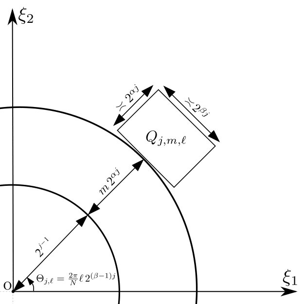 Figure 1
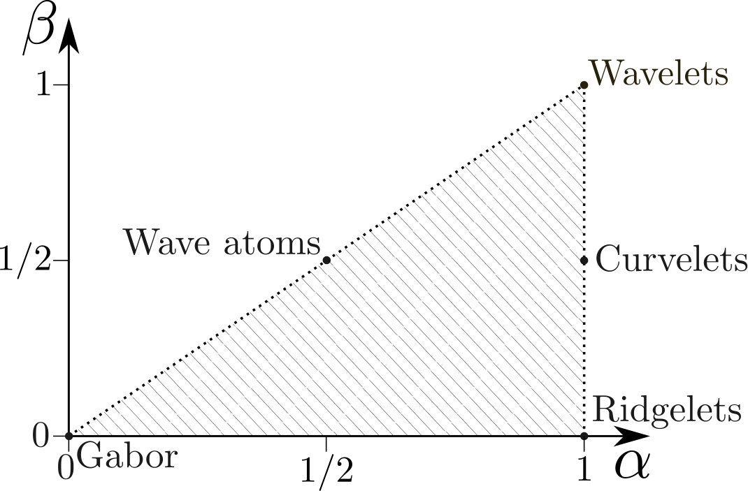 Figure 2