Counting perfect matchings and the eight-vertex model
Jin-Yi Cai, Tianyu Liu

TL;DR
This paper investigates the computational complexity of approximating the partition function of the eight-vertex model on 4-regular graphs, establishing connections to the hard problem of counting perfect matchings and providing new characterizations of matchgates.
Contribution
It relates the approximability of the eight-vertex model to counting perfect matchings and characterizes nonnegative 4-ary matchgates, extending previous complexity results.
Findings
Approximation of the partition function is as hard as counting perfect matchings in certain parameter regions.
Computing the partition function can be reduced to counting perfect matchings in larger parameter regions.
Identifies a parameter region where planar graph approximation is feasible but general graph approximation is as hard as counting perfect matchings.
Abstract
We study the approximation complexity of the partition function of the eight-vertex model on general 4-regular graphs. For the first time, we relate the approximability of the eight-vertex model to the complexity of approximately counting perfect matchings, a central open problem in this field. Our results extend those in arXiv:1811.03126 [cs.CC]. In a region of the parameter space where no previous approximation complexity was known, we show that approximating the partition function is at least as hard as approximately counting perfect matchings via approximation-preserving reductions. In another region of the parameter space which is larger than the previously known FPRASable region, we show that computing the partition function can be reduced to (with or without approximation) counting perfect matchings. Moreover, we give a complete characterization of nonnegatively weighted (not…
Click any figure to enlarge with its caption.
 Figure 1
 Figure 2
 Figure 3
 Figure 4
 Figure 5
 Figure 6
 Figure 7
 Figure 8
 Figure 9
 Figure 10
 Figure 11
 Figure 12
 Figure 13
 Figure 14
 Figure 15
 Figure 16
 Figure 17
 Figure 18
 Figure 19
 Figure 20
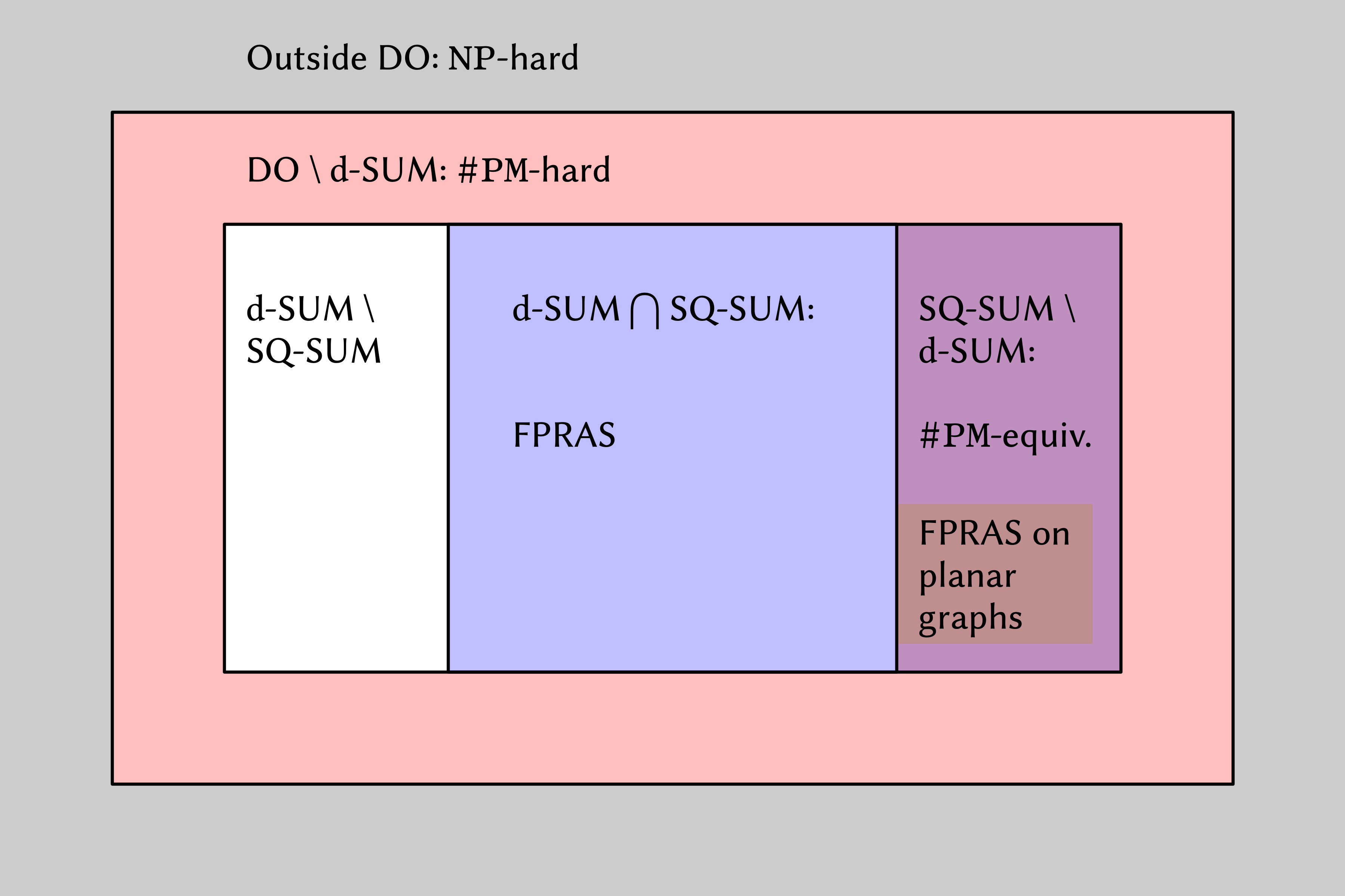 Figure 21
 Figure 22
 Figure 23
 Figure 24
 Figure 25
 Figure 26
 Figure 27
 Figure 28
 Figure 29
 Figure 30
 Figure 31
 Figure 32
 Figure 33
 Figure 34
 Figure 35
 Figure 36
 Figure 37
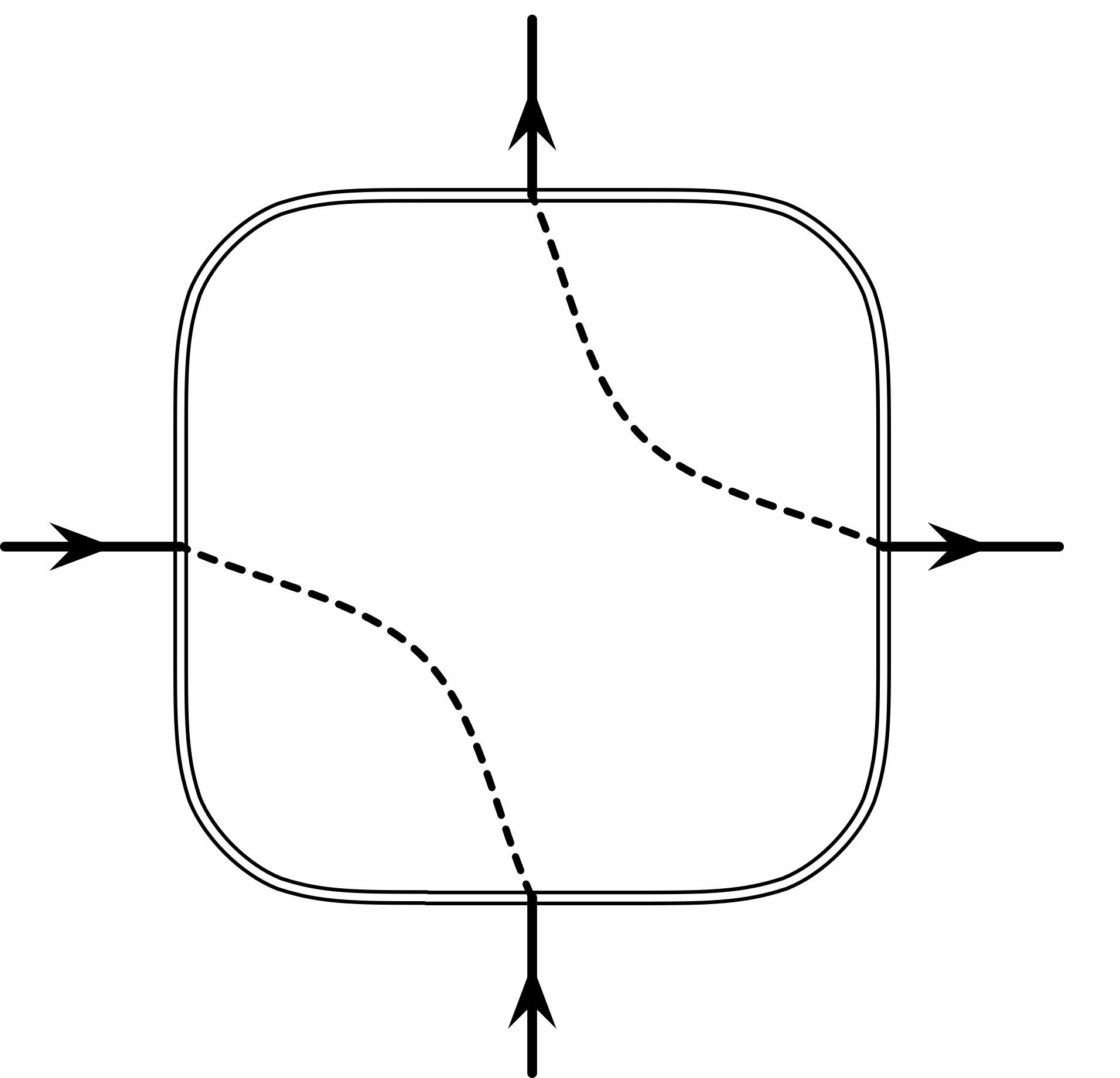 Figure 38
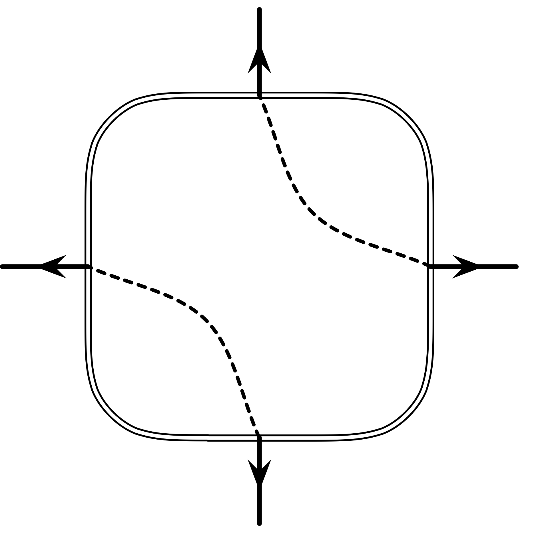 Figure 39
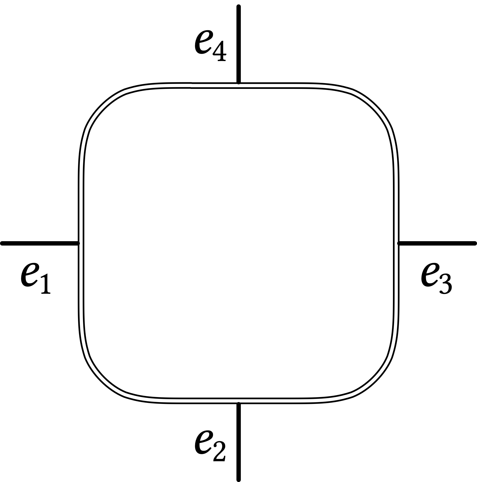 Figure 40
Peer Reviews
No public reviews on file for this paper yet. If you reviewed it on a platform where reviews are public (OpenReview, ICLR, NeurIPS, ICML), you can paste yours below so the community can read it here.
Videos
No videos yet. Explain this paper in a talk, walkthrough, or lecture? Add one.
Counting perfect matchings and the eight-vertex model
Jin-Yi Cai Department of Computer Sciences, University of Wisconsin-Madison. Supported by NSF CCF-1714275. [email protected]
Tianyu Liu Department of Computer Sciences, University of Wisconsin-Madison. Supported by NSF CCF-1714275. [email protected]
Abstract
We study the approximation complexity of the partition function of the eight-vertex model on general 4-regular graphs. For the first time, we relate the approximability of the eight-vertex model to the complexity of approximately counting perfect matchings, a central open problem in this field. Our results extend those in [CLLY18].
In a region of the parameter space where no previous approximation complexity was known, we show that approximating the partition function is at least as hard as approximately counting perfect matchings via approximation-preserving reductions. In another region of the parameter space which is larger than the previously known FPRASable region, we show that computing the partition function can be reduced to (with or without approximation) counting perfect matchings. Moreover, we give a complete characterization of nonnegatively weighted (not necessarily planar) 4-ary matchgates, which has been open for several years. The key ingredient of our proof is a geometric lemma.
We also identify a region of the parameter space where approximating the partition function on planar 4-regular graphs is feasible but on general 4-regular graphs is equivalent to approximately counting perfect matchings. To our best knowledge, these are the first problems of this kind.
1 Introduction
The eight-vertex model is defined over 4-regular graphs, the states of which are the set of even orientations, i.e. those with an even number of arrows into (and out of) each vertex. There are eight permitted types of local configurations around a vertex—hence the name eight-vertex model (see Figure 1).
Classically, the eight-vertex model is defined by statistical physicists on a square lattice region where each vertex of the lattice is connected by an edge to four nearest neighbors. In general, the eight configurations 1 to 8 in Figure 1 are associated with eight possible weights . By physical considerations, the total weight of a state remains unchanged if all arrows are flipped, assuming there is no external electric field. In this case we write , , , and . This complementary invariance is known as arrow reversal symmetry or zero field assumption.
Even in the zero-field setting, this model is already enormously expressive: its special case when , the zero-field six-vertex model, has sub-models such as the ice (), KDP, and Rys models; on the square lattice, some other important models such as the dimer and zero-field Ising models can be reduced to it [Bax72]. After the eight-vertex model was introduced in 1970 by Sutherland [Sut70], and Fan and Wu [FW70], Baxter [Bax71, Bax72] achieved a good understanding of the zero-field case in the thermodynamic limit on the square lattice (in physics it is called “exactly solved”).
In this paper, we assume the arrow reversal symmetry and further assume that , as is the case in classical physics. Given a 4-regular graph , we label four incident edges of each vertex from 1 to 4. The partition function of the eight-vertex model with parameters on is defined as
[TABLE]
where is the set of all even orientations of , and is the number of vertices in type in (, locally depicted as in Figure 1) under an even orientation .
In terms of the exact computational complexity, a complexity dichotomy is given for the eight-vertex model on 4-regular graphs for all eight parameters [CF17]. This is studied in the context of a classification program for the complexity of counting problems [CC17], where the eight-vertex model serves as important basic cases for Holant problems defined by not necessarily symmetric constraint functions. It is shown that every setting is either P-time computable (and some are surprising) or #P-hard. However, most cases for P-time tractability are due to nontrivial cancellations. In our setting where are nonnegative, the problem of computing the partition function of the eight-vertex model is #P-hard unless: (1) (this is equivalent to the unweighted case); (2) at least three of are zero; or (3) two of are zero and the other two are equal. In addition, on planar graphs it is also P-time computable for parameter settings with , using the FKT algorithm.
Since exact computation is hard in most cases, one natural question is what is the approximate complexity of counting and sampling of the eight-vertex model. To our best knowledge, prior to [CLLY18], there is only one previous result in this regard due to Greenberg and Randall [GR10]. They showed that on square lattice regions a specific Markov chain (which flips the orientations of all four edges along a uniformly picked face at each step) is torpidly mixing when is large. It means that when sinks and sources have large weights, this particular chain cannot be used to approximately sample eight-vertex configurations on the square lattice according to the Gibbs measure. Recently, similar torpid mixing results have been achieved for the six-vertex model on the square lattice [Liu18].
[CLLY18] gave the first classification results for the approximate complexity of the eight-vertex model on general and planar 4-regular graphs, and they conform to phase transition in physics. This is an extension to the work on the approximability of the six-vertex model [CLL19]. In order to state the results in [CLLY18] and in this work, we adopt the following notations assuming .
- •
DO = ;
- •
-SUM = ;
- •
SQ-SUM = .
Remark 1.1*.*
-SUM , SQ-SUM .
Physicists have shown an order-disorder phase transition for the eight-vertex model on the square lattice between parameter settings outside DO and those inside DO (see Baxter’s book [Bax82] for more details). In [CLLY18], it was shown that: (1) approximating the partition function of the eight-vertex model on general 4-regular graphs outside DO is NP-hard, (2) there is an FPRAS‡‡‡Suppose is a function mapping problem instances to real numbers. A fully polynomial randomized approximation scheme (FPRAS) [KL83] for a problem is a randomized algorithm that takes as input an instance and , running in time polynomial in (the input length) and , and outputs a number (a random variable) such that for general 4-regular graphs in the region -SUM SQ-SUM, and (3) there is an FPRAS for planar 4-regular graphs in the extra region SQ-SUM.
In this paper we make further progress in the classification program of the approximate complexity of the eight-vertex model on 4-regular graphs in terms of the parameters (see Figure 2). For the first time, the complexity of approximating the partition function of the eight-vertex model (#EightVertex()) is related to that of approximately counting perfect matchings (#PerfectMatchings).
Theorem 1.1**.**
For any four positive numbers such that (a,b,c,d)\not\in\textup{{d-SUM}}, the problem #EightVertex() is at least as hard to approximate as counting perfect matchings:
[TABLE]
Remark 1.2*.*
The theorem is stated for the case where all four parameters are positive. The same proof also works for the case when there is exactly one zero among the nonnegative values . A complete account for four nonnegative values is given in the Appendix A.
The proof of Theorem 1.1 is in Section 3. Our proof for the hardness result has several ingredients:
- (1)
We express the eight-vertex model on a 4-regular graph as an edge-2-coloring problem on using Valiant’s holographic transformation [Val08]. 2. (2)
We show that some special cases in this edge-2-coloring problem on is equivalent to the zero-field Ising model on its crossing-circuit graph . Thus known #PerfectMatchings-equivalence result for the Ising model [GJ08, Lemma 7] directly transfers to the special cases under certain parameter settings. 3. (3)
We further show that for any parameter setting outside -SUM, approximating the partition function of the eight-vertex model is at least as hard as the #PerfectMatchings-equivalent special cases of the edge-2-coloring problem via approximation-preserving reductions (introduced in [DGGJ04]).
Theorem 1.2**.**
For any ,
[TABLE]
The proof of Theorem 1.2 is in Section 4. To prove the easiness result, we again express the eight-vertex model in the Holant framework (see Section 2) and show that the constraint functions of the eight-vertex model in SQ-SUM can be implemented by constant-size matchgates with nonnegatively weighted edges (Definition 4.1). We note that allowing nonnegative edge-weights does not add more computational power [McQ13, Proposition 5]. The crucial ingredient of our proof is a geometric lemma (Lemma 4.3) in 3-dimensional space.
Our result is tight in the sense that no constraint functions of the eight-vertex model with parameter settings outside the region SQ-SUM can be implemented by a matchgate (Lemma 4.4). Moreover, the general version of our result also works for the eight-vertex model without the arrow reversal symmetry. It is open if computing the partition function in \texttt{DO}\setminus(\texttt{d-SUM}\bigcup\texttt{SQ-SUM}) is #PerfectMatchings-equivalent or not.
As part of this work, we give a complete characterization of the constraint functions that can be expressed by 4-ary matchgates in Theorem 4.1. This solves an important question that has been open for several years [McQ13, BGJ*+*17]. We believe it is of independent interest.
Corollary 1.3**.**
For any four positive numbers such that (a,b,c,d)\in\textup{{SQ-SUM}}\setminus\textup{{d-SUM}},
[TABLE]
Note that for the eight-vertex model in the region SQ-SUM, computing is (1) #P-complete in exact computation [CF17], (2) #PerfectMatchings-equivalent in approximate computation on general 4-regular graphs (Corollary 1.3), and (3) admits an FPRAS in approximate computation on planar 4-regular graphs [CLLY18]. To our best knowledge, these are the first identified problems of this kind.
2 Preliminaries
Given a 4-regular graph , the edge-vertex incidence graph is a bipartite graph where is an edge in iff in is incident to . We model an orientation () on an edge from into in by assigning to and [math] to in . A configuration of the eight-vertex model on is an edge 2-coloring on , namely , where for each its two incident edges are assigned 01 or 10, and for each the sum of values , over the four incident edges of . Thus we model the even orientation rule of on all by requiring “two-0-two-1/four-0/four-1” locally at each vertex .
The “one-0-one-1” requirement on the two edges incident to a vertex in is a binary Disequality constraint, denoted by . The values of a 4-ary constraint function can be listed in a matrix , called the constraint matrix of . For the eight-vertex model satisfying the even orientation rule and arrow reversal symmetry, the constraint function at every vertex in has the form , if we locally index the left, down, right, and up edges incident to by 1, 2, 3, and 4, respectively according to Figure 1. Thus computing the partition function is equivalent to evaluating
[TABLE]
where denotes the incident edges of . In fact, in this way we express the partition function of the eight-vertex model as the Holant sum in the framework for Holant problems:
[TABLE]
where we use to denote the Holant sum on a bipartite graph for the Holant problem . Each vertex in (or ) is assigned the constraint function (or , respectively). The constraint function is considered as a row vector (or covariant tensor), whereas the signature is considered as a column vector (or contravariant tensor). (See [CC17] for more on Holant problems.) The following proposition says that an invertible holographic transformation does not change the complexity of the Holant problem in the bipartite setting.
Proposition 2.1** ([Val08]).**
Suppose is an invertible matrix. Let and . Define and . Then for any bipartite graph , .
3 #PerfectMatchings-hardness
Our proof strategy for Theorem 1.1 is as follows. In Lemma 3.1, we express the eight-vertex model on a 4-regular graph as a Holant problem; this is an equivalent form of the orientation problem expressed as an edge-2-coloring problem on , and is achieved using a holographic transformation. In Lemma 3.3, we establish the equivalence between some special cases of this edge-2-coloring problem and the zero-field Ising model. Thus a known result for the Ising model (Proposition 3.2) indicates the #PerfectMatchings-equivalence of the special cases under certain parameter settings (Corollary 3.4). It follows from Lemma 3.5 that for any with (and symmetrically or ), approximately computing the partition function is at least as hard as the #PerfectMatchings-equivalent special cases under approximation-preserving reductions.
Lemma 3.1**.**
.
Proof.
Using the binary disequality function for the orientation of any edge, we can express the partition function of the eight-vertex model as a Holant problem on its edge-vertex incidence graph ,
[TABLE]
where is the 4-ary constraint function with . According to Proposition 2.1, under a -transformation where , we have
[TABLE]
and a direct calculation shows that . ∎
Proposition 3.2** ([GJ08, Lemma 7]).**
Suppose . Then .
Lemma 3.3**.**
The Ising problem is equivalent to the Holant problem . In particular, .
Remark 3.1*.*
A non-homogenized form of the Ising model is . If then . If then in all vertices in each component must take the same assignment (all [math] or all ). In this case both and the Holant problem in Lemma 3.3 are trivially solvable in polynomial time.
Proof.
For the problem , the roles of are interchangeable by relabeling the edges. For example, if the constraint function has the constraint matrix , then the constraint function has the constraint matrix . It follows that
[TABLE]
are exactly the same problem. So to prove the lemma it suffices to prove the equivalence of
[TABLE]
First we show that can be expressed as
Given a 4-regular graph as an instance of , we can partition into a set of circuits (in which vertices may repeat but edges cannot) in the following way: at every vertex , denote the four edges incident to by in a cyclic order according to the local labeling of the signature function; we make and into adjacent edges in a single circuit, and similarly we make and into adjacent edges in a single circuit (note that these may be the same circuit). We say each circuit in is a crossing circuit of . For the graph , we define its crossing-circuit graph , with possible multiloops and multiedges, as follows: its vertex set consists of the crossing circuits; for every , if circuits and intersect at , then there is an edge labeled by . Note that it is possible that , and for such a self-intersectison point the edge is a loop. Each may have multiple loops, and for distinct circuits and there may be multiple edges between them. The edge set of is in 1-1 correspondence with of .
Observe that the problem requires that every valid configuration (that contributes a non-zero term) obeys the following rule at each vertex :
- •
Assuming are the four edges incident to in cyclic order, then (denoted by ) and (denoted by ). That is to say, all edges in a crossing circuit must have the same assignment (either all [math] or all ). Therefore, the valid configurations on the edges of are in 1-1 correspondence with -assignments on the vertices of .
- •
Under , the local weight on is if and is otherwise. Suppose crossing circuits and intersect at (they could be identical). Then in , has local weight on the edge if and has local weight otherwise.
This means
[TABLE]
Next we show that can be expressed as Note that every graph (without isolated vertices) is the crossing-circuit graph of some 4-regular graph . To define from , one only needs to do the following: (1) transform each vertex into a closed cycle ; (2) for each loop at , make a self-intersection on ; and (3) for each non-loop edge ( and are two distinct vertices), make and intersect in a “crossing” way at a vertex in (by first creating a vertex on and another vertex on , then merging and with local labeling on and on ). Then the above proof holds for the reverse direction. ∎
Corollary 3.4**.**
Suppose and . Then
Lemma 3.5**.**
Suppose and at most one of is zero. Then .
Proof.
According to Lemma 3.1, we only need to prove
[TABLE]
Figure 3 describes a simple gadget construction in the Holant framework. In Figure 3 if we place the constraint function with and with at the two degree 4 vertices, then the constraint function of the 4-ary construction is . Since
[TABLE]
we know that the Holant problem below on the left can be expressed by the Holant problem on the right, and therefore
[TABLE]
Notice that is the signature matrix of the arity 4 equality function . Therefore, (3.1) is true if we can show
[TABLE]
which is equivalent to the following in the orientation view according to the proof of Lemma 3.1
[TABLE]
by the holographic transformation
[TABLE]
a constant multiple of the even parity function, which has the signature matrix .
Next we show how to get (3.2). Given the constraint function with matrix in #EightVertex(), we construct a 4-ary signature with constraint matrix using a polynomial number of vertices and edges such that , , , and are all exponentially close to after normalization, i.e., to be close to 1, for any , with a construction of size in polynomial time.
We assume we start with the following condition:
[TABLE]
If this is not the case, we can obtain a 4-ary construction that realizes this condition using constantly many vertices. With some preliminary construction we can further assume initially. (See Appendix B for details.) Note that starting with the constraint function with matrix , we can arbitrarily permute by relabeling the edges, and so we get constraint functions with and with . There are two constructions and which we use as basic steps; both constructions start with a constraint function with parameters satisfying (3.3).
: connect two vertices with constraint functions and respectively as in Figure 3. Since we are in the orientation view, we place the constraint function on the two degree 2 vertices connecting the two degree 4 vertices. Then the constraint function of the construction is obtained by matrix multiplication , where . Thus
[TABLE]
The constraint function has four new parameters, denoted by
[TABLE]
We make the following observations; all of them can be easily verified using (3.3):
- •
is the weight on sink and source and .
- •
.
- •
.
- •
because . 2. 2.
: connect two vertices with constraint functions as in Figure 3. Denote the constraint function of by . We have
[TABLE]
The constraint function has four new parameters, denoted by
[TABLE]
The following observations can also be easily verified using (3.3):
- •
is the weight on sink and source and if , then .
- •
.
- •
.
Based on the two basic constructions above, we construct the constraint function in logarithmically many rounds recursively, each of the rounds uses the constraint function constructed in the previous round. We now describe a single round in this construction, which consists of two steps. In step 1 we use a signature with some parameter setting satisfying (3.3) and apply to two copies of the signature. If the resulting parameter we switch the roles of and , and obtain , again satisfying (3.3), as well as . In step 2, we apply to two copies of the signature constructed in step 1 (with the switching of the roles of and if it is needed). Denote the parameters of the resulting signature by . Altogether each round uses four copies of the signature from the previous round, starting with the initial given signature. Therefore in polynomial time we can afford to carry out rounds for any constant . Note that, if we consider the normalized quantities , then the respective quantities in each step and do not increase their distances to 1, i.e.,
[TABLE]
This is true even if the construction in step 2 is applied in the case when the roles of and are switched for the signature from step 1, when that switch is required () as described. More importantly, based on the properties of and , we know that the (normalized) gap between and the previous largest entry shrinks quadratically fast, as measured by the new normalized with . More precisely,
[TABLE]
Note that may no longer be the largest among ; however we will permute them to get so that (3.3) is still satisfied before proceeding to the next round. This completes the description of our construction in one round which obtains from .
We will construct the final signature by rounds of this construction. Also we will follow each value individually as they get transformed through each round. To state it formally, starting with the normalized triple , we define a successor triple , so that each entry has the respective successor (e.g., the entry has successor ). This is well-defined because and are homogeneous functions of . Note that even though from one round to the next, we may have to rename so that the permutated triple satisfies (3.3), the successor sequence as the rounds progress stays with an individual value. E.g., starting from , if after one round , then the successor of after two rounds is . Now define to be the (ordered) triple , or its successor triple, at the beginning of the -th round, for .
Let be the 4-ary signature constructed after rounds. By the Pigeonhole Principle, after rounds, at least one of has the property that in at least many rounds the corresponding or its successors are the maximum (normalized) value in that round, and thus its next successor gets shrunken quadratically in that round. Suppose this is ; the same proof works if it is or . Let be the maximum (normalized) value at the beginning of round in rounds, where , and . Since initially we have ,
[TABLE]
Then
[TABLE]
By induction . At the end of rounds, if has parameters , then
[TABLE]
Therefore, after logarithmically many rounds, using polynomially many vertices, we can get a 4-ary construction with parameters , , , and that are exponentially close to 1 after normalizing by . Thus (3.2) is proved. ∎
4 #PerfectMatchings-easiness
In this section, we address two problems:
What are the constraint functions that can be realized by 4-ary matchgates (Definition 4.1)?
Although the set of constraint functions that can be realized by planar matchgates with complex edge weights have been completely characterized [CC17], the set of constraint functions that can be realized by general (not necessarily planar) matchgates with nonnegative real edge weights is not fully understood, even for matchgates of arity 4. This type of matchgates plays a crucial role in the study of the approximate complexity of counting problems, as we will see in this paper.
In Theorem 4.1, we give a complete characterization of constraint functions of arity 4 that can be realized by matchgates with nonnegative real edges. Our method is primarily geometric. 2. 2.
Theorem 1.1 shows that for positive parameters (a,b,c,d)\not\in\texttt{d-SUM} the problem #EightVertex() is at least as hard as counting perfect matchings approximately. Here we ask the reverse question: For what parameter settings does #EightVertex() #PerfectMatchings?
We know that
[TABLE]
where is the 4-ary constraint function with . Considering the fact that can be easily realized by a matchgate (a vertex with two dangling edges), Theorem 1.2 is a direct consequence of Lemma 4.2 which says that any constraint function in SQ-SUM is realizable by some 4-ary matchgate of constant size (with nonnegative edge weights, but not necessarily planar) (see Definition 4.1). Our theorem works for the eight-vertex model with parameter settings (defined below) not necessarily satisfying the arrow reversal symmetry.
Moreover, Lemma 4.4 indicates that our result is tight in the sense that captures precisely the set of all constraint functions that can be realized by 4-ary matchgates (with even support, i.e., nonzero only on inputs of even Hamming weight). A similar statement holds for . the corresponding set with odd support.
Definition 4.1**.**
We use the term a -ary matchgate to denote a graph having “dangling” edges, labelled . Each dangling edge has weight and each non-dangling edge is equipped with a nonnegative weight . A configuration is a -assignment to the edges. A configuration is a perfect matching if every vertex has exactly one incident edge assigned . The matchgate implements the constraint function , where for is the sum, over perfect matchings, of the product of the weight of edges with assignment , where the dangling edge is assigned , and the empty product has weight .
Remark 4.1*.*
Contrary to Definition 4.1 which does not require planarity, planar matchgates with complex edge weights has been completely characterized [Val02, CC17]. As computing the weighted sum of perfect matchings is in polynomial time over planar graphs by the FKT algorithm [TF61, Kas61, Kas67], problems that can be locally expressed by planar matchgates are tractable over planar graphs.
Notation*.*
, .
Theorem 4.1**.**
Denote by the set of constraint functions that can be realized by 4-ary matchgates. Then .
Remark 4.2*.*
Note that any constraint function in must satisfy either even parity (nonzero only on inputs of even Hamming weight) or odd parity (nonzero only on inputs of odd Hamming weight). Theorem 4.1 for the even parity part () is a combination of Lemma 4.2 and Lemma 4.4. The odd parity part can be proved similarly.
Lemma 4.2**.**
Suppose . Then there is a 4-ary matchgate of constant size whose constraint function is .
Proof.
We first note that if any of the four inequalities in the definition of is an equality, then the remaining three inequalities automatically hold, since the 8 values are all nonnegative.
Given a constraint function , first we construct a matchgate for . If then all four products , and one can easily adapt from the following proof to show that the signature is realizable as a matchgate signature. So it suffices to implement the normalized version . Our construction is a weighted depicted in Figure 4a. Let be the dangling edges incident to vertices , respectively. Denote by the weight on the edge between vertex and vertex . One can check that the following weight assignment meets our need: .
For , without loss of generality we assume and we normalize . Then our construction is shown in Figure 4b where we set . One can verify that it realizes the normalized constraint function . The construction for and are symmetric to the above case.
It remains to show that the interior
[TABLE]
can all be reached. We first deal with the case when all eight parameters are strictly positive and leave the other cases to the end of this proof. We use a weighted to be our matchgate depicted in Figure 4c, and set . Then the matchgate has a singature with the following parameters
[TABLE]
Note that all the edge weights have to be nonnegative. By properly setting the edge weights in the matchgate, we show that we can achieve any relative ratios among the eight given positive values that satisfy (4.1). Our first step is to achieve any relative ratios among the four product values , , , satisfying (4.1); and the second step is to adjust the relative ratio within the pairs , , and without affecting the product values. This can be justified by the observation that, by a scaling a global positive constant can be easily achieved, and all appearances of and in (4.1) are as a product , and similarly for .
For the fourteen edge weights to be determined, let
[TABLE]
and define
[TABLE]
Note that are all nonnegative and so are .
Our goal is to choose the fourteen edge weights so that are all positive and satisfy
[TABLE]
Note that, by definition, the left-side of (4.4) is precisely the right-side of (4.4) when are replaced by respectively. Denote the products by respectively. Then (4.4) is a set of four linear equations , where . Note that is invertible and , so (4.4) is equivalent to , having an identical form. Since the requirement (4.1) in terms of translates into the requirement being strictly positive via , it is not surprising that the requirement being strictly positive translates into the requirement
[TABLE]
and that are positive is the same as (4.1).
Furthermore, let , then the requirement being positive is equivalent to the requirement . This is because is the same as .
The crucial ingredient of our proof is a geometric lemma in 3-dimensional space. Suppose are positive and they satisfy (4.1). This defines . By a scaling we may assume . Hence are positive and satisfy (4.5). Thus belongs to the set in the statement of Lemma 4.3.
By Lemma 4.3, there exist (strictly) positive tuples and such that
[TABLE]
satisfying and . By the previous observation this indicates that there exist (strictly) positive such that .
We first set so that for some constant . To achieve this, set , and let be positive, and then set , , , and . We have , and . Then set , which can be independently any positive numbers at least 2, by choosing to be suitable positive numbers. This allows us to get such that for some constant . Then it is obvious that can be set so that . Compute according to (4.3). As a consequence, is a valid solution.
To adjust the relative ratio between , say increasing by , while keeping all product values and the relative ratios within the other three pairs, just increase by and increase by . Similarly, to increase by alone without affecting the other products and ratios, just increase by and by , and decrease by and by . The other cases are symmetric.
Finally we deal with the cases when there are zeros among the eight parameters. Note that at most one of is zero, because if at least two products are zero, say , then (4.1) forces a contradiction that and . In the case :
- •
: We make the modification that , i.e. .
- •
: We make the further modification that .
- •
: We connect the four dangling edges in Figure 4c to four degree 2 vertices, respectively. This switches the role of and in the previous proof.
One can check our proof is still valid in the above three cases. If , then we connect the dangling edges on vertices 1, 2 to two degree 2 vertices (similar to the operation from Figure 4a to Figure 4b). This switches the role of with and the proof folllows. The proofs for and are symmetric. ∎
Now we give the crucial geometric lemma.
Lemma 4.3**.**
Let , , and . Then is the Minkowski sum of and , namely, consists of precisely those points , such that for some and . The same statement is true for the closures of , and .
Proof.
Observe that , , and are the interiors of a polyhedron with 7 facets, a regular triangle, and a polyhedron with 3 facets, respectively.
The polyhedron for is the intersection of three half spaces bounded by three planes, , where the planes are defined by equalities. Note that these inequalities imply that , thus this polyhedron has only three facets. We can find the intersection of each pair of the three planes for as . Note that these intersections lie on the planes , , and , respectively.
Let . Then the triangle for is just the convex hull of . Suppose we shift the origin of from to and denote the resulting (interior of a) polyhedron by , then we have the defining inequalities , where the shifted planes are defined by the corresponding equalities. By symmetry, if we shift the origin of to and to , we have respectively with , and with . Note that the shifted planes , , and contain three distinct facets of , and they coincide exactly with a facet of , , and , respectively.
By sliding with its origin along the line from to , we have a partial coverage of by the shifting copies of from and :
- •
The shifted ray of moves from to . Notice that this is a parallel transport, and stays on the plane , and thus it swipes another facet of on bounded by the two lines and .
- •
The shifted ray of moves from to ; the shifted ray of moves from to . Notice that both stay on the plane which is .
It follows that the part of satisfying is covered by the Minkowski sum of and the line segment on from to (which is a side of the triangle ).
Symmetrically, after sliding with its origin from to along the line we get the parallel tranport from to . Also after sliding with its origin from back to along the line segment we get the parallel tranport from to . After these, the only subset in that is left uncovered by shifting copies of is — a tetrahedron (Figure 5b). However this subset can be covered by the rays . Note that for all . This completes the proof. ∎
Lemma 4.4**.**
Suppose is the constraint function of a 4-ary matchgate with . Then . In particular, if satisfies arrow reversal symmetry, .
Remark 4.3*.*
The last part was proved in [BGJ*+*17, Lemma 56]. The proofs for other three parts are symmetric and similar to the proof for the last part. For completeness, here we give the proof for the first part .
Proof.
Consider a 4-ary matchgate with constraint function . Given that , is equivalent as
[TABLE]
Let be the set of dangling edges of . For , let denote the set of perfect matchings that include dangling edges in (by assigning them ) and exclude dangling edges in (by assigning them [math]). We exhibit an injective map
[TABLE]
which is weight-preserving in the sense that for matchings with , we have . The existence of implies (4.6).
Given , consider and note that this is a collection of cycles together with two paths. Let be the path connecting the dangling edge to some other dangling edge; let be the path connecting the remaining two dangling edges. Let and . Then we have the following
- •
If connects to , then and ;
- •
If connects to , then and ;
- •
If connects to , then and .
The construction is invertible, since if is in the image of the above mapping, then . From , we can recover (as the unique path that connects to one of the other dangling edges in ). Then we can recover and as and respectively. Therefore, is an injection.
To see that is weight-preserving, observe that the each of the edges in appears in exactly one of and and in exactly one of and and that for . Hence,
[TABLE]
∎
Appendix
Appendix A
Appendix B
Given a constraint function with and , we show how to obtain a 4-ary construction with constraint function such that and satisfy the condition , using copies of the constraint function . (When used in the context of Lemma 3.5, the number of copies of used is a constant.) By a scaling we get
[TABLE]
We first deal with the case where one of is equal to 0. By relabeling we may assume . Then we use the construction in the proof of Lemma 3.5 to get a signature with parameters with no zero entries.
In the following we may assume all entries are positive .
Our first step is to satisfy (3.3). If all four entries are equal then we are done (the signature is also in the affine family and thus the problem is also P-time tractable.) So we may assume at least one of . By relabeling we may assume . We may also assume at least one of the following three displayed inequalities does not hold, and by relabeling we may assume . Indeed, if all three inequalities
[TABLE]
hold, then by connecting two copies of using the 4-ary construction in Figure 3 and relabeling edges, we get . This signature has .
Under a holographic transformation (in the proof of Lemma 3.1), in the edge-2-coloring view becomes , where . Connect copies of using the 4-ary construction in Figure 3, we get the constraint function with which in the edge-2-coloring view becomes . By construction, it is also equal to
[TABLE]
It follows that
[TABLE]
Since is strictly larger than , and also and , one can see that for a large , we can get such that , and all entries are positive. If furthermore , then we have arrived at a signature satisfying (3.3) with a possible relabeling. If , using the construction in Figure 3 with two copies of (and two in the middle as we are in the orientation view), we can get with . The four parameters for is which satisfies (3.3) (with a possible relabeling) when .
Now that we have a constraint function (or if the last step is needed) satisfying (3.3), we obtain using 4-ary constructions with (or respectively). This is done by repeatedly applying (defined in Lemma 3.5) in which each round starts with the function constructed from the previous round, and possibily relabeling the input values , so that the construction starts with some satisfying (3.3). Note that for any satisfying (3.3) and , shrinks the distance between and by at least a constant (after normalization). This can be checked by when . Therefore, starting with and iterative applying (constantly many times), we can obtain so that .
The reference list from the paper itself. Each links out to its DOI / PubMed record.
- 1[Bax 71] R. J. Baxter. Eight-vertex model in lattice statistics. Phys. Rev. Lett. , 26:832–833, Apr 1971.
- 2[Bax 72] R. J. Baxter. Partition function of the eight-vertex lattice model. Annals of Physics , 70(1):193 – 228, 1972.
- 3[Bax 82] R. J. Baxter. Exactly Solved Models in Statistical Mechanics . Academic Press Inc., San Diego, CA, USA, 1982.
- 4[BGJ + 17] Andrei Bulatov, Leslie Ann Goldberg, Mark Jerrum, David Richerby, and Stanislav Živný. Functional clones and expressibility of partition functions. Theoretical Computer Science , 687:11 – 39, 2017.
- 5[CC 17] Jin-Yi Cai and Xi Chen. Complexity Dichotomies for Counting Problems , volume 1. Cambridge University Press, 2017.
- 6[CF 17] Jin-Yi Cai and Zhiguo Fu. Complexity classification of the eight-vertex model. Co RR , abs/1702.07938, 2017.
- 7[CLL 19] Jin-Yi Cai, Tianyu Liu, and Pinyan Lu. Approximability of the six-vertex model. In Proceedings of the Thirtieth Annual ACM-SIAM Symposium on Discrete Algorithms , SODA ’19, pages 2248–2261, 2019.
- 8[CLLY 18] Jin-Yi Cai, Tianyu Liu, Pinyan Lu, and Jing Yu. Approximability of the eight-vertex model. Co RR , abs/1811.03126, 2018.