From coupled-wire construction of quantum Hall states to wave functions and hydrodynamics
Y. Imamura, K. Totsuka, T.H. Hansson

TL;DR
This paper links the coupled wire construction of Abelian quantum Hall states with composite boson theory to derive wave functions and hydrodynamic descriptions, including the Wen-Zee action, providing a new constructive approach.
Contribution
It introduces a method to extract Laughlin wave functions and hydrodynamic theories directly from the coupled wire construction, enhancing understanding of topological quantum Hall states.
Findings
Derived Laughlin wave function from coupled wire model
Reconstructed Wen-Zee topological action in bulk
Provided a recipe for general Abelian quantum Hall states
Abstract
In this paper we use a close connection between the coupled wire construction (CWC) of Abelian quantum Hall states and the theory of composite bosons to extract the Laughlin wave function and the hydrodynamic effective theory in the bulk, including the Wen-Zee topological action, directly from the CWC. We show how rotational invariance can be recovered by fine-tuning the interactions. A simple recipe is also given to construct general Abelian quantum Hall states desceibed by the multi-component Wen-Zee action.
Click any figure to enlarge with its caption.
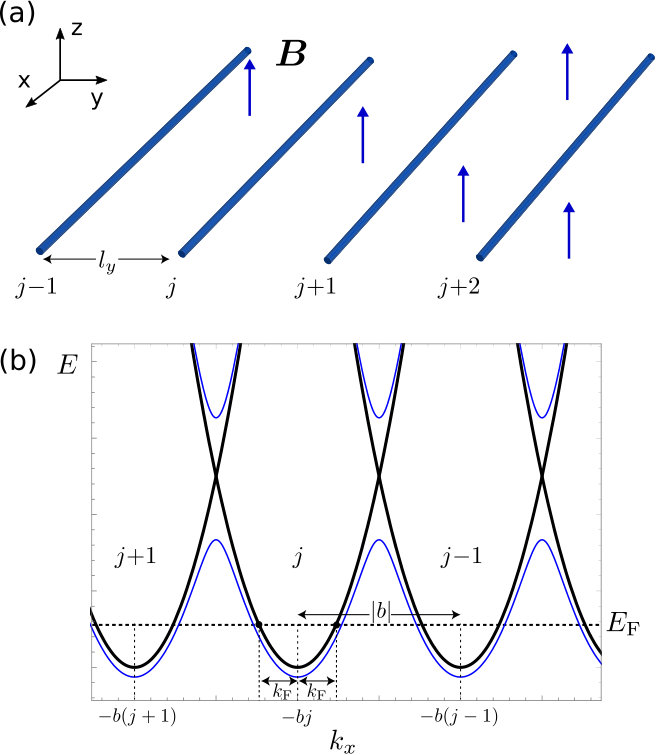 Figure 1
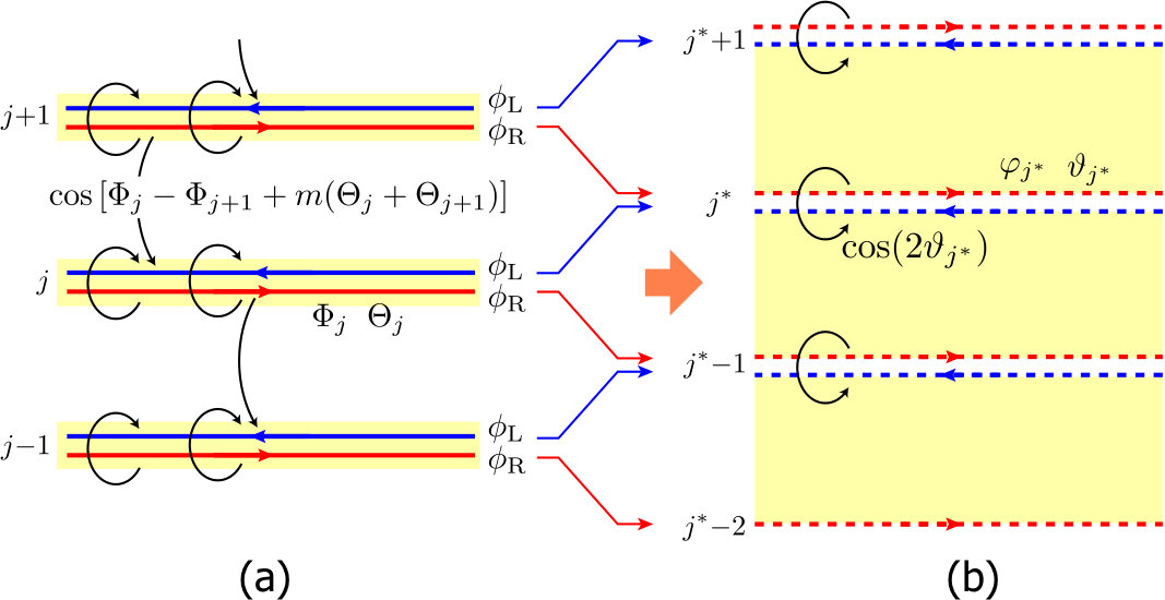 Figure 2
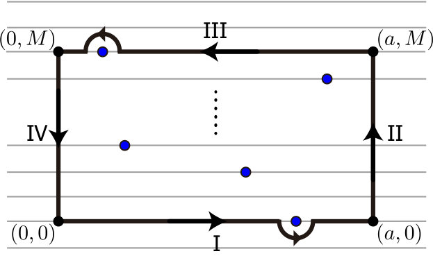 Figure 3
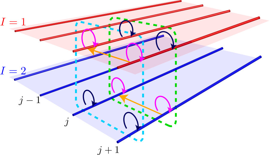 Figure 4
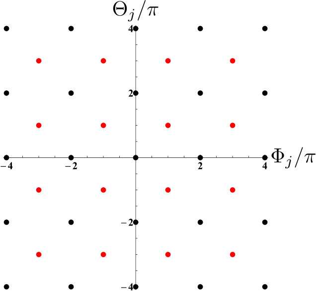 Figure 5
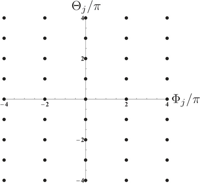 Figure 5
Peer Reviews
No public reviews on file for this paper yet. If you reviewed it on a platform where reviews are public (OpenReview, ICLR, NeurIPS, ICML), you can paste yours below so the community can read it here.
Videos
No videos yet. Explain this paper in a talk, walkthrough, or lecture? Add one.
From coupled-wire construction of quantum Hall states to wave functions and hydrodynamics
Yukihisa Imamura
Division of Physics and Astronomy, Graduate School of Science, Kyoto University, Kyoto 606-8502, Japan.
Yukawa Institute for Theoretical Physics, Kyoto University, Kyoto 606-8502, Japan
Keisuke Totsuka
Yukawa Institute for Theoretical Physics, Kyoto University, Kyoto 606-8502, Japan
T.H. Hansson
Yukawa Institute for Theoretical Physics, Kyoto University, Kyoto 606-8502, Japan
Department of Physics, Stockholm University, AlbaNova University Center, SE-106 91 Stockholm, Sweden
Abstract
In this paper we use a close connection between the coupled wire construction (CWC) of Abelian quantum Hall states and the theory of composite bosons to extract the Laughlin wave function and the hydrodynamic effective theory in the bulk, including the Wen-Zee topological action, directly from the CWC. We show how rotational invariance can be recovered by fine-tuning the interactions. A simple recipe is also given to construct general Abelian quantum Hall states described by the multi-component Wen-Zee action.
I Introduction
Topological order Wen (2004) is one of the most fundamental concepts in modern condensed matter physics. The history starts with the discovery of the fractional quantum Hall effect (FQHE) in the 1980’s *Tsui *et al. (1982), which was essentially understood after Laughlin proposed his famous wave function Laughlin (1983). Since then, theorists have proposed a variety of topologically ordered states in two and three dimensions. Examples in dimensions are Abelian hierarchical quantum Hall (QH) states Haldane (1983); Halperin (1984); Jain (2007), non-Abelian QH states Moore and Read (1991); Read and Rezayi (1999), and various kinds of spin liquids Kalmeyer and Laughlin (1987); *Wen *et al. (1989); Wen (1991); Moessner and Sondhi (2001); Kitaev (2003); Levin and Wen (2005). Some, but far from all, of these states have strong experimental support.
Topologically ordered states are featureless and symmetric in the bulk, and as such they defy the characterization of phases by local order parameters in the manner of Landau. Nevertheless, there are field theoretic descriptions. It is belived that the topological properties can be encoded in various types of topological field theories, the most well known examples being the Chern-Simons theories of the QHE Blok and Wen (1990); Wen and Zee (1992a).
Going beyond the topological scaling limit Fröhlich and Kerler (1991), but still in the infrared region, there are hydrodynamical descriptions that supplement the topological action with higher-order derivative terms. These theories typically encode information about collective excitations. Yet another type of field theories are those based on statistical transmutation, or “flux attachment”. These theories of “composite” fermions Lopez and Fradkin (1991) or bosons *Zhang *et al. (1989), which are closely related to various model wave functions, are in principle microscopic, but can only be solved using various kinds of mean-field approximations.
In addition to the various field theories, there are several other ways to describe topologically ordered states in general, and quantum Hall states in particular. Examples of the latter are the approach based on the thin-torus limit Bergholtz and Karlhede (2008), and the coupled wire construction (CWC) of Kane and coworkers *Kane *et al. (2002); Teo and Kane (2014). The aim of this paper is to make a rigorous connection between this last approach and the Chern-Simons field-theory for composite bosons.
The CWC is quite general, and has been employed to construct various two- and three-dimensional topological states. The list includes the original work on Abelian and non-Abelian fractional quantum Hall states *Kane *et al. (2002); Teo and Kane (2014); Fuji and Lecheminant (2017), chiral spin liquid states *Meng *et al. (2015), topological insulators and superconductors in two- and three dimensions Sagi and Oreg (2015); *Santos *et al. (2015); Sagi and Oreg (2014); *Seroussi *et al. (2014), and the construction of higher-dimensional Abelian topological phases *Iadecola *et al. (2016). A re-derivation of the periodic table of integer and fractional fermionic topological phases was given in *Neupert *et al. (2014). In this paper, we shall only consider Abelian QH states, and in particular the Laughlin states.
The essence of the CWC is to build interacting fermion/boson systems by starting from a collection of parallel “wires” in a strong magnetic field, each one supporting a Luttinger liquid. The wires are then coupled by tunneling interactions, and there are also forward scattering interactions on each wire that couple right and left moving electrons. Keeping only the intra-wire current-current interactions, the system is in the so-called sliding Luttinger liquid phase *Kivelson *et al. (1998); *O’Hern *et al. (1999); *Emery *et al. (2000); *Mukhopadhyay *et al. (2001); Vishwanath and Carpentier (2001) and remains invariant under independent global U(1) transformations and translations on each wire.
A key observation is that inter-wire interactions can be used to freeze most of the above symmetry. Kane et al. *Kane *et al. (2002), showed that, in the limit of strong inter-wire coupling, and at certain rational filling fractions, one retains various two-dimensional ground states whose properties depend on the the details of the construction. In the simplest case of the Laughlin state, it is sufficient to couple neighboring wires, but in general several wires have to be coupled.
The CWC gives an intuitive description of the chiral edge states in a way resembling the occurrence of fractional spins at the ends of the Affleck-Kennedy-Lieb-Tasaki chain *Affleck *et al. (1988), or of Majorana modes at the ends of a Kitaev chain Kitaev (2001). The basic mechanism is that the right and left-moving electrons on neighboring chains pair, leaving a right-moving channel on one side of the sample and a left-moving one on the other. One can also show that the number of degenerate ground states are as expected, and that the kink excitations on the wires indeed are the fractionally charged anyons characteristic of FQH liquids.
It is less clear how the CWC, which, by definition, explicitly breaks rotational invariance, will describe other characteristics of the Laughlin states, such as its wave function and collective excitations. In this paper, we reformulate the CWC in terms of gauge fields, in a way that makes it clear how to reproduce the known bulk properties. Not surprisingly, a fine-tuning of a parameter is needed to get an isotropic two-dimensional liquid, but we also show that the topological properties do not depend on this. Concretely, we shall use the bosonic fields in the CWC to define a gauge field that can be identified with the statistical gauge field in the Chern-Simons-Ginzburg-Landau (CSGL) theory of the Laughlin states *Zhang *et al. (1989); Zhang (1992). Using this, we derive the Laughlin wave function, both in the isotropic and anisotropic cases, and the hydrodynamic effective theory which contains the Wen-Zee topological action Wen and Zee (1992a) as its leading term in a derivative expansion.
A comment is in order about an interesting recent paper by Fuji and Furusaki Fuji and Furusaki (2019). In fact, there is an overlap in the underlying idea between it and this work. Rather than directly identifying the composite-boson field in the CWC, they explicitly carry out the flux attachment on the wires, and then add an interaction term that stabilizes the superfluid phase of the composite bosons. Finally, using a coupled-wire version of the boson-vortex duality transformation Fisher and Lee (1989), they arrive at an action that couples the dual (vortex) fields, describing the quasiparticles, to a hydrodynamic gauge field with a Chern-Simons action. Despite similar looking, this theory differs in some important respects from the hydrodynamic effective theory we shall derive below. We comment on this in the end of Sec. V. Also, fluctuations and the wave function, which are main subjects of this paper, are not discussed in Ref. Fuji and Furusaki (2019).
The paper is organized as follows. We begin by briefly reviewing the CWC in Sec. II and show how to identify the physically inequivalent ground states. In Sec. III, we define a gauge field which can be interpreted as a statistical gauge field and explain the connection to the CSGL theory. Section IV contains the derivation of the Laughlin wave function starting from our effective Hamiltonian, as well as a discussion of the effects of the spatial anisotropy which is naturally present in the coupled wires. In Sec. V, we derive the hydrodynamical theory, that contains the topological Wen-Zee action, from the effective action obtained in the previous section and show that the Kohn mode is correctly reproduced. The generalization to arbitrary Abelian states is given in Sec. VI, and we end with a concluding section. Some technicalities are summarized in two Appendices.
II Laughlin state in Coupled Wire Construction
The Laughlin state is the paradigmatic example of topological states of matter (see, e.g., Refs. Jain, 2007; Hansson **et al., 2017 for reviews of the Laughlin and other quantum Hall states). The defining properties of the state are encoded in the Wen-Zee topological action which is a level- U(1) Chern-Simons gauge theory Blok and Wen (1990); Lopez and Fradkin (1991). The corresponding edge theory is a chiral Luttinger liquid, which is a chiral boson compactified on a circle with radius Wen (1990). We now review the CWC for the Laughlin state following the original work by Kane et al. *Kane *et al. (2002).
II.1 From uncoupled to to coupled wires
Consider a set of parallell one-dimensional wires running along the direction and stacked in the direction with a distance [see Fig. 1(a)]. We then apply a strong magnetic field which is perpendicular to the plane and is given by the gauge potential (Landau gauge). We consider non-relativistic spinless fermions (with mass ) moving on the wire with the dispersion relation , where [see Fig. 1(b); for electrons]. When these bands are filled up to the Fermi momentum [see Fig. 1(b)], the fermion density on each wire is given by , and this gives the filling fraction: . When , the Fermi points are located exactly at the lowest crossing points and the inclusion of the single-particle hopping among the neighboring wires opens a band gap there, which is identified with one of the gaps separating the (quasi-one-dimensional) Landau levels as is seen in the thin curves in Fig. 1(b).
At a filling fraction, , which is relative to the filled Landau levels, the single-particle hopping never opens a gap at the Fermi points and we need interactions to make the system gapped. To develop a systematic approach, we linearize the low-energy dispersion around the Fermi points and to obtain two Dirac fermions , and respectively, which are related to the original spin less fermion as:
[TABLE]
The low-energy effective Hamiltonian for the -th wire is given by that of massless Dirac fermion:
[TABLE]
where the velocity is common to all wires. (To ease the notations, we set in what follows.)
By Abelian bosonization Giamarchi (2004), the chiral spinless fermions and on each wire () are expressed, at low energies, in terms of the chiral bosons as
[TABLE]
where are the Klein factors necessary to guarantee the anti-commutation among the spinless fermions on different wires. The symbol denotes the normal-ordering necessary to regularize the operator-products; to simplify the notations, we suppress it hereafter. In terms of the bosonic fields (compactified on a circle with radius ) and their duals
[TABLE]
the low-energy effective Hamiltonian for the spinless fermion is
[TABLE]
where is the number of wires in the stacking () direction. The bosonic fields satisfy
[TABLE]
and the Luttinger liquid parameter equals to 1 for free fermions but, in general, and are renormalized in the presence of interactions. The field is related to the particle density [measured from its average ] on the -th wire:
[TABLE]
This relation will be used frequently in the following sections.
To introduce interactions, we consider an adjacent pair, e.g., and . In order to gap out most of the degrees of freedom and leave gapless chiral Luttinger liquids only at the edges, the authors of Refs. *Kane *et al. (2002); Teo and Kane (2014) introduced the following, carefully designed, inter-wire interaction allowed by U(1) and translation symmetries:
[TABLE]
where is an odd integer for fermions 111At this stage, must be integer as the number of back-scattered fermions must be integer: . However, once the interaction is given in terms of bosons and as in Eq. (9), we can think of bosonic problem with even-..
This interaction is made up of two simultaneous -pled (on-wire) backscattering processes on the adjacent wires and inter-wire single-particle hopping (i.e., consists of -particle processes). According to Eq. (1), the chiral fermions and are accompanied, respectively, by the oscillating factors and . Therefore, if we construct the interaction from the original -fermions, it must contain the factor . Requiring to be non-oscillatory (i.e., translationally invariant) fixes the filling fraction .
In terms of the bosonic fields, reads as 222 We were not precise about the ordering of the fermion operators in (8); we assume that they are correctly ordered in such a way that, when bosonized, they reproduce (9).
[TABLE]
where lives on the “fictitious” wire (or strip) located in the middle of the two wires and (see the dashed lines in Fig. 2). Physically, the part comes from the single-particle hopping between neighboring wires, and from the tailored backscattering within individual chains *Kane *et al. (2002); Teo and Kane (2014). The new fields may be viewed as parts of a new set of bosons on strips (see Fig. 2)
[TABLE]
that, from (6), obey the following commutation relation:
[TABLE]
They may be viewed as made up of the new set of “chiral bosons”
[TABLE]
as and .
In the strong-coupling limit , the bosonic fields are pinned at one of the minima of the cosine potential,
[TABLE]
where . Any semi-classical ground state is then specified by a set of integers . However, all these states, labeled by , are not physically distinct, since, as will be shown in the next section, some of them must be identified up to the periodicity of the bosonic fields and .
II.2 Ground-state degeneracy
One of the crucial signatures of a topologically ordered state in dimensions is the ground state degeneracy on higher-genus surfaces. The simplest non-trivial example is the -fold degeneracy in the Laughlin states Haldane and Rezayi (1985); Wen and Niu (1990). In the strong-coupling limit, the (semi-classical) CWC ground states are found by minimizing the potential with respect to , and there seems to be infinitely many of them labeled by the set of integers in (13). Reference Teo and Kane (2014), gave an argument about the ground-state degeneracy based on the limit . Here we count the number of inequivalent ground states by taking into account the periodic structure of the bosonic fields *Lin *et al. (1998); Lecheminant and Totsuka (2006). As the derivation is straightforward but slightly involved, we just give a sketch here and the details, for both fermions and bosons, are given in Appendix A.
First, we assume that the system is defined on a torus and impose periodic boundary condition both in the wire () direction and in the stacking direction (, ). One may think that the wires are infinitely long and that the geometry of the system is cylindrical. However, the argument (in Appendix A) relies essentially on the structure of the zero modes which is peculiar to periodic systems (see, e.g., Fig. 5), and we implicitly assume the periodicity in the direction as well.
Then we use the expressions (3) expressing the Dirac fermions in terms of the bosons to infer that states which differ by a shift of must be identified:
[TABLE]
(Bosons have a different periodicity, as explained in Appendix A.) Due to the periodicity, most of the would-be ground states are equivalent. In fact, as proven in Appendix A, any pair of ground states and are equivalent and represent the same physical state if, and only if,
[TABLE]
Thus we conclude that in the coupled-wire system with strong inter-wire interaction (9), there are precisely distinct ground states that are characterized by:
[TABLE]
From the above, it follows that the eigenvalues of the Wilson loop operator
[TABLE]
distinguish the different ground states. Then, by using Eq. (11), we readily see that the operator
[TABLE]
changes the eigenvalue of by and creates a different ground state. Since, according to the arguments in Ref. Teo and Kane (2014), the operator may be viewed as transporting a quasi-particle along the wire , this perfectly agrees with the well-known picture that the insertion of fluxes, corresponding to quasi-particle transport around non-trivial loops, generates topologically different ground states Wen and Niu (1990).
III From Coupled wires to Chern-Simons theory
The argument in Sec. II.2 already suggests us to identify with a gauge-like degree of freedom. In this section, we proceed along this line to identify the bosonic fields with the statistical gauge field.
III.1 Introducing gauge fields
Since -dependent local gauge transformations of fermions, , change the boson field as , it is natural to identify
[TABLE]
as the component of a two dimensional gauge field. To obtain a bona fide two-dimensional gauge field, we also need the component, and to this end, we note that transforms as the component of a lattice gauge field. To see this, recall that a link variable transforms as 333 Note that the -dimension is continuous while the -dimension is discrete. This can be thought of a an Euledian version of the Kogut-Susskind formulation of lattice gauge theory Kogut and Susskind (1975).
[TABLE]
where the lattice spacing is the distance between the wires. This implies
[TABLE]
which suggests us to identify with a proper choice of gauge. In the continuum where we put , the component reads as:
[TABLE]
Combining (19) and (22), we obtain the following gauge field:
[TABLE]
which, by Eq. (6), satisfies the commutation relation:
[TABLE]
This can also be derived from a theory with a Chern-Simons term
[TABLE]
in the Lagrangian, which is precisely how the statistical gauge field appears in the Chern-Simons-Ginzburg-Landau (CSGL) theory *Zhang *et al. (1989). That the normalization of is consistent with this interpretation is seen by calculating the statistical magnetic field
[TABLE]
where we have used Eq. (7) and that the two-dimensional density () is related to the one-dimensional one by . Equation (26) implies that fluxes are attached to each electron thereby confirming our interpretation.
An attentive reader should have noticed that in the above argument, the normalization of was of central importance. For instance, renormalizing the relation (23) by a factor would have given a coefficient in the CS Lagrangian (25), and in that case it would have been tempting to identify with the hydrodynamical field in the Wen-Zee theory of quantum Hall liquids Wen and Zee (1992a). However, in the next subsection we show that our identification of as a statistical gauge field is indeed the correct one.
A remark on the strong-coupling limit is in order. In the usual treatment of the CWC, the strong-coupling limit is used to simply gap out all the bulk degrees of freedom leaving the gapless modes only at the boundaries. Here, as we shall see, the strong-coupling limit enters via the consistency with the continuum limit. In Ref. *Santos *et al. (2015), an infinitely strong inter-wire interaction locks an external electromagnetic field to . For the external gauge field to be completely canceled by the statistical gauge field, which is the essence of the mean-field approximation in the CSGL theory, the coupling must be strong. In the CSGL theory, the large energy scale is the cyclotron energy in the uncancelled magnetic field, while in our case it is the inter-wire coupling .
III.2 Relation to the CSGL theory
So far, we have considered only the extreme strong-coupling limit where is strictly pinned to the minimum of the cosine potential. Relaxing this condition, and also retaining the terms from the Luttinger Hamiltonian (5), we get the effective Hamiltonian for the field
[TABLE]
where we used the mean-field relation , with the external magnetic field and the mean area density, to rewrite the Fermi velocity as . Here, is the cyclotron energy ( is the electron band mass), and we introduced the dimensionless coupling strength by,
[TABLE]
In the last term in (27), which comes from the term in the Luttinger Hamiltonian (5), denotes the deviation from the average area density .
So far, and are free parameters but we shall now impose the condition which ensures rotational invariance in (27). It should be no surprise that fine tuning is needed to retain rotational invariance; it is in fact more surprising that rotational invariance can at all be recovered in the CWC. In order for the continuum approximation to make sense [for ], we must take to be small and thus must be large , albeit not infinite. The rotationally invariant effective Lagrangian now reads as
[TABLE]
This is not a topological field theory since the leading term () in a derivative expansion does depend on the metric. Thus we could not have interpreted as the hydrodynamical field even if we had changed the normalization to get the “correct” CS term.
It is illuminating to compare this with the standard CSGL theory given by the Lagrangian *Zhang *et al. (1989); Zhang (1992),
[TABLE]
where is a composite boson minimally coupled to the external electromagnetic gauge field , is a statistical gauge field, and is a repulsive two-body repulsive potential.
We proceed by first parametrizing the bosonic field as
[TABLE]
and then integrate out the non-dynamical field to get the constraint , where is the flux of the statistical gauge field , and the chemical potential is such that has a minimum at . Neglecting derivatives of the density, making the mean-field approximation , and assuming a local potential , we get
[TABLE]
with . To derive this result, we absorbed the gradient of the phase, , in the vector potential , which amounts to picking a unitary gauge.
Recalling that , (29) and (32) become identical if we take (i.e., ), identify in (29) as the fluctuation in the statistical gauge field, and pick in the CSGL theory (32) to match the coefficient in front of in the CWC expression. In what follows, we fix and except in Sec. VI. This equivalence is a main result of this paper, and it shows that, after introducing interactions, the bosons on the wires become bona fide composite bosons.
Having shown the equivalence between the CWC and the CSGL theory, it is reasonable to expect that the results from the latter can be derived also in the present context. In the next two sections, we shall show that this is indeed the case. Before doing so, however, we shall make some comment about the edge modes.
The presence of chiral gapless edge modes is at the heart of the CWC. The way the right and left moving modes on the adjacent wires are coupled is designed in such a way that the correct chiral modes are left at the wires at the edges of the system. It is clearly of importance that our continuum description in terms of gauge fields is able to describe these modes as well. In fact, as we already advertised, we will eventually derive the Wen-Zee theory, which is known to give a correct description of the edge Wen (1995). Turning to the intermediate theory given by (29), one might naively expect that there are no gapless modes because of the quadratic terms.
IV The Laughlin wave function from coupled wires
In this section, we derive the Laughlin wave function from the CWC. We do it first for the (fine-tuned) rotationally invariant theory (29), and then for the general anisotropic case.
IV.1 The isotropic case
In the standard derivation *Kane *et al. (1991); Zhang (1992) of the wave function from the CSLG theory, one uses the Coulomb gauge and rewrites the Hamiltonian as a collection of harmonic oscillators in the variables and . One then finds the wave function for the composite bosons, by using the density representation of the wave functional. Finally, the full lowest-Landau-level Laughlin wave function is regained by reintroducing the phase factor that was taken out in the statistical transmutation from the original electrons to the composite bosons. In the present context, the derivation of the norm of the wave functions only differs from the standard CSGL procedure by some technicalities, while that for the phase requires a careful treatment, and provides a non-trivial consistency check of our calculations.
Instead of the Coulomb gauge, we are implicitly using the unitary gauge, where the phase fluctuations are absorbed in the gauge field [see, e.g., Eq. (32)], and our treatment here also differs from that in the standard CSLG treatment in that the relation between and the density is anisotropic as is seen in Eq. (26). With this in mind, we proceed by making the following decomposition for :
[TABLE]
so that . Substituting (33) in the Lagrangian density (29) gives the Lagrangian,
[TABLE]
where we have set and used that, by partial integration, the cross terms between and vanish in the Hamiltonian part while the diagonal terms vanish in the kinetic term. Using , we see that and are conjugate variables satisfying . The Hamiltonian becomes,
[TABLE]
where we used and only kept the leading terms in a derivative expansion. In the density () representation, the wave functional is that of an assembly of harmonic oscillators labeled by . Using the explicit non-relativistic form of the density operator, with being the position of the electron, and the mean density which is related to the magnetic length by , the wave function reads as
[TABLE]
In the above, we have used the complex notaion , and we refer to Refs. *Kane *et al. (1991); Zhang (1992) for details of the derivation.
The Laughlin wave function differs from (36) by the phase factor
[TABLE]
in which exchanging two electrons yields a phase angle , while transporting one around another yields . We now show that we can reconstruct the additional phase factor (37) within the CWC by carefully calculating the Berry phase factor acquired when transporting an electron along the path shown in Fig. 3. In doing so, we first calculate the phase using Eq. (37). When moving along the paths I and III, the transported electron exchanges its position with other electrons sitting on the wires 0 and thereby acquiring the phase each time (in the Laughlin state). On the segments II and IV, on the other hand, there are no exchanges. Nevertheless, the full loop encircles all the electrons sitting on the wires 1 to and picks up the phase from each electron. If we define to denote the ground-state expectation value of the operator , then, by Eq. (7), the number of electrons in the interval of the wire is given by . Combining all this, we expect the total phase acquired by the electron:
[TABLE]
To calculate the Berry phase related to transporting a right-moving electron (we could equally well have considered a left mover) within the CWC, we first define the states:
[TABLE]
where and is the ground state. We have also introduced the notation to avoid clutter. The Berry connection is defined by:
[TABLE]
where we used that, because of reflection symmetry when , there is no -component of the current in the ground state: , and properly regularized the product . It is now easy to calculate the Berry phase corresponding to the segment I:
[TABLE]
In the same way, we get for the segment III:
[TABLE]
Along to the segment II, we shall return to the original discretized formulation and define the the Berry phase factor as we do in lattice field theories
[TABLE]
with
[TABLE]
where we used that on different wires commute. The next, and crucial, step is to rewrite the exponent in (44) as,
[TABLE]
where we have suppressed the dependence. We now recall, from Sec. II.1, that is pinned to a constant , which we take to be zero (as mod , we arrive at the same phase factor for any other choices; the important thing is that it does not depend on the geometry of the loop). Adding the contributions from all the wires () together and taking the expectation value, we are left with the phase:
[TABLE]
The segment IV gives a similar expression, now evaluated at , and with an additional minus sign. Putting everything together, and taking into account that the Berry phase differs by a sign from the exchange phase calculated from the wave function *Hansson *et al. (1990), we obtain precisely the phase (38) that was derived from (36). Note that, only after carefully taking into account both the phases from the particle exchange on the loop and from the encircled charges inside, we obtained the correct result.
Because of the close analogy to the CSGL theory, it is natural to expect that the above derivation can also be modified to give the wave functions of the Laughlin holes. We shall not elaborate on the details, but just make two observations. First, adding a kink on the wire in the loop in Fig. 3, will, by exactly the same argument as above, give the Berry phase (38) without thereby leading to an extra phase factor:
[TABLE]
where . Since it will also give a contribution [] to the density operator , it is easy to see that it will add the correct modulus which, together with the above phase factor, reproduces the correct Laughlin hole factor .
The quasielectrons are harder to deal with. Although it is straightforward to calculate the fractional charges and the statistical phase factors for states with anti-kinks on the wires, it is non-trivial to extract wave functions. This asymmetry in the description of quasiholes and quasielectrons is well-known both in the CSGL theory, and in approaches based on conformal field theory *Hansson *et al. (2017).
IV.2 The anisotropic case
If we do not make the (fine-tuned) choice , that is necessary to get the isotropic theory (29), the Hamiltonian will depend on the combination
[TABLE]
with . Since and , a rescaling implies,
[TABLE]
Alternatively, we could rescale and . In both cases, the terms change as:
[TABLE]
while remains invariant. Thus, if we use the primed coordinates, the previous derivation of the Laughlin wave function will go through without any changes, while the complex coordinate will be redefined as . In terms of the wave functions in the lowest Landau level, this amounts to having coherent states which are not circular, but deformed into ellipses. As has been stressed by Haldane Haldane (2011) and others *Suorsa *et al. (2011); *Hansson *et al. (2017), the Laughlin state is more general in nature than its usual incarnation as a holomorphic polynomial in .
V The topological and hydrodynamic actions
Here we derive the effective hydrodynamical theory which contains the Wen-Zee topological field theory as the leading term in the infrared. From this, we extract the collective Kohn mode and its dispersion. We also show how to couple the hydrodynamic theory to an external perturbing electromagnetic field.
V.1 The topological action
When doing the gauge transformation
[TABLE]
the CS Lagrangian (25) picks up an extra piece , and, using the notation , we can recast it into the relativistic form,
[TABLE]
If we introduce a new gauge field , the partition function for this CS theory can be rewritten as follows,
[TABLE]
where , and with
[TABLE]
Integrating out the statistical gauge field in (52) yields the constraint (remember that the background charge has been subtracted already) leaving only the first term which is precisely the Wen-Zee topological action for the Laughlin state.
The Wen-Zee action is trivial on an infinite plane, but codes for the -fold ground-state degeneracy on higher-genus () surfaces, as well as giving the kinetic term for the chiral edge modes Wen (1995). The ground state degeneracy is consistent with the counting done in Sec. II.2, and the presence of chiral edge modes in the direction of the wires was a starting point of the CWC *Kane *et al. (2002).
The fact that the Wen-Zee action follows from the CWC strongly suggests that there will be gapless edge modes also in the perpendicular direction in the case of finite length wires with open boundary conditions. However, we do not claim to have proven this since the derivation of the topological action did not incorporate open boundary conditions in the -direction. Here, a comment on the edge Hamiltonian is in order. From the CWC perspective, the edge modes parallel to the wires are nothing but the decoupled chiral components at the outermost wires. As such, they have a Hamiltonian given explicitly by the chiral Luttinger theory which is at the basis of the construction. In particular, the velocity depends explicitly on the topological number . There is no reason to believe that this would give a good description of a real QH edge, where the edge velocity is known to depend on the edge potential. Thus, the edge velocity should be considered as an extra phenomenological parameter, and the same holds for the multi-component case discussed in Sec. VI.
V.2 The hydrodynamical action and the Kohn mode
In the previous section, we only retained the topological part (25) of the full action (29). We now show that, by including the Hamiltonian part, we can complement the Wen-Zee topological term with higher derivative contributions that describe collective modes. To this end, we begin with the low-energy effective Lagrangian (29):
[TABLE]
where we have added the term to retain the correct constraint. Following the same logic as in the previous section, but with replaced by the above expression, we first integrate out the density fluctuations to get a term in the action:
[TABLE]
where we defined the dimensionless parameter and used the relation .
As above, we then proceed to integrate the field to get the desired effective hydrodynamic theory:
[TABLE]
where and are the field strengths related to .
It is now straightforward to extract the dispersion relation for the collective mode described by the dynamics of this effective theory,
[TABLE]
This should be compared with the result from the CSGL theory (30) Lee and Zhang (1991); Zhang (1992):
[TABLE]
where is the Fourier transform of the two-body potential . We see, as expected from (29) and (32), that the result from the coupled wire construction correspond to having a delta function potential.
V.3 Coupling to an external electromagnetic field
So far we did not include the coupling to electromagnetism, except for the constant field that determines the ground state density . Minimal coupling of electromagnetism to a phase field is implemented by the standard substitution,
[TABLE]
and recalling the definition (23), this implies that is incorporated by the substitution in the Hamiltonian, and is coupled by adding the term to (53). With this in mind, the Lagrangian (54) generalizes to,
[TABLE]
[Note that the substitution (58), which amounts to a minimal coupling, should be done only in the Hamiltonian; the CS action, which encodes the proper commutation relations, is not to be changed.] By a shift, , the integration over can be performed as in the previous section, and we regain the result (55) with the extra term
[TABLE]
which is the desired coupling of the electromagnetic potential to the conserved current .
At this point, it behooves us to clarify the relation to the approach by Fuji and Furusaki in Ref. Fuji and Furusaki (2019). Our hydrodynamic Lagrangian (55), supplemented by the electromagnetic coupling (60), should be compared with their Eq. (52). They use the notation for our hydrodynamic gauge field and also consider couplings to a bosonic quasiparticle described by . As they point out, their final expression contains a term that may be obtained by discretizing the topological part of (55). However, it crucially differs from (55) in that the field does not have any dynamics, and that Eq. (52) has other terms that may eventually generate more relevant contributions (e.g., ) in a derivative expansion.
VI General abelian QH states
Having understood how a topological quantum field theory emerges from the CWC in the simplest case of the Laughlin states, we now ask what in the previous analysis will carry over to general abelian QH states which are described by the Wen-Zee Lagrangian Wen and Zee (1992a):
[TABLE]
In the above, are Chern-Simons gauge fields, and the “ matrix”, , is symmetric and integer-valued. The integer-valued “charge vector”, determines how the th component of the U(1) charge couples to the external elcetromagnetic field Wen (1995). The topological field theories of the form (61) are known to describe not only genuine topological phases Wen and Zee (1992a) but also symmetry-protected ones Lu and Vishwanath (2012). In Ref. Teo and Kane (2014), Teo and Kane gave a construction for the simple case of a matrix. Their method generalizes quite straightforwardly to a general matrix, and so does the extraction of the topological field theory (61).
To closely follow the steps given in Sec. II.1 for the single component case, we prepare layers of coupled wires and define the following bosons as in Eq. (12),
[TABLE]
where we have introduced the vectorial notations, e.g.,
[TABLE]
Each pair of bosons obey the commutation relations (6) and describe a Luttinger liquid on the wire- of the th layer (see Fig. 4) with the Luttinger parameter . From these fields, we define the following bosons living on the strip :
[TABLE]
Note that the on-strip fields are not local in that they contain on different layers as well as on the same layer.
Again in analogy with the single component case, it is clear that to reproduce the Wen-Zee action (61) we need the following interactions between the adjacent wires,
[TABLE]
Following the procedure given in Ref. Teo and Kane (2014), we find that, in the strong-coupling limit of , there are gapless modes at the lower edge described by the following edge Hamiltonian
[TABLE]
and similarly for the upper edge . If we identify the non-universal velocity matrix as:
[TABLE]
the edge Hamiltonian (66) coincides with that predicted by the hydrodynamic Chern-Simons action (61) Wen (1995). As has been remarked in Sec. V.1, that the matrix, which is of purely topological origin, appears in the edge Hamiltonian (66) through the non-universal velocity is just an artifact of using the special inter-wire interaction (65) to construct the QH state.
Then, by properly identifying the statistical gauge fields , we can derive the Wen-Zee action (61) with . Since we follow almost the same steps as before, we just sketch the derivation in Appendix B.2. Also it is not hard to use the method in Sec. V.2 to calculate the higher-derivative corrections to the topological action (61) but we do not give the details here. The construction here uses the multi-layer setting. However, as is described in Appendix B.3, we can always recast the multi-layer system into a single-layer one with longer-range interactions as in Ref. Teo and Kane (2014).
It is straightforward to rewrite (65) in terms of suitably ordered interactions among fermions or bosons that generalize (8). In fact, as is shown in Appendix B.1, in order for the above interactions to be written only in terms of local operators of the original fermionic/bosonic theories, the matrix must satisfy
[TABLE]
Recovering all the Klein factors (in the fermion case) and combining (68) with the relation derived from the commutation relations, we see that, for both fermions and bosons, all the terms in (65) are commuting and can be minimized simultaneously.
By requiring translational invariance of the inter-wire interactions, we can determine the filling at which these interactions are allowed. The magnetic field and the particle density of each layer may be recovered by the following substitution for all layers and wires ,
[TABLE]
Then, the inter-wire interactions (65) acquire additional dependence in the cosines. The translational invariance requires that these oscillating factors should vanish:
[TABLE]
From this, we can read off the corresponding filling fraction as:
[TABLE]
Comparing this with the general expression from the Chern-Simons theory , we see that our construction corresponds to the symmetric basis Wen (1995). Although it is rather straightforward, we will not derive the ground-state degeneracy along the lines in Sec. II.2 444Now the equivalence relation corresponding to (15) is
with a set of vectors defined by . That is, if the difference between any given pair of ground states is on the lattice spanned by , they are equivalent. Then, the volume of a unit cell of this lattice gives the ground-state degeneracy., since the result also follows directly from the effective Wen-Zee theory (61) to be derived in Appendix B.2 Keski-Vakkuri and Wen (1993); *Wesolowski *et al. (1994).
Regarding the wave functions, there is an important distinction between states formed by multicomponent states where the particles are distinguishable by spin or some “layer” index Girvin and MacDonald (1997), and where they are indistinguishable, as in the hierarchy of spin-polarized states in the lowest Landau level. In the first case, which includes the Halperin states Halperin (1983), one can derive the wave functions using the same technique as in Sec. IV. The hierarchy wave functions pose a much more difficult problem. Here, the electrons in the layers (or effective Landau levels in the language of composite fermions) are distinguished by their orbital spin. This is a topological quantity that is most directly revealed by geometrical response, since it couples to external curvature Wen and Zee (1992b), but it is also related to the Hall viscosity which is a transport coefficient Read (2009). It is a challenge to to incorporate the orbital spin in the CWC.
VII Summary and outlook
In this paper we have considered the bulk properties in the CWC, i.e., the (topological) ground-state degeneracy, the wave function, the bulk effective theory, and the low-energy excitations. In the limit of sufficiently strong inter-wire interactions, the ground states are found by minimizing the interaction energy. We gave, for the Laughlin states, the precise condition to identify physically inequivalent ground states and showed that the CWC correctly reproduces the number of degenerate ground states on a torus.
In order to describe the low-energy properties in the bulk, we first identified the bosons on the wires as composite bosons and found the expressions for the statistical gauge field in the CSGL theory. These enabled us to obtain the low-energy effective action for the statistical (Chern-Simons) gauge field, from which we constructed the bulk Laughlin wave function within the framework of the CWC. By integrating out the statistical gauge field, we then derived the hydrodynamic effective action (the Maxwell-Chern-Simons theory) in which the leading term is the topological Wen-Zee action. We also discussed the effects of anisotropy, which is inherent in the CWC, on the bulk properties. The methods developed for the simplest Laughlin states were readily generalized to give a simple recipe for constructing general Abelian quantum Hall states, characterized by a matrix, and the corresponding multi-component Wen-Zee action.
Our work points at several directions that might be fruitful to explore. In the CWC, it is by its nature quite easy to find the gapless edge modes at the boundaries parallel to the wires. Although we derived the bulk Wen-Zee action that does encode the chiral edge states at any boundaries, it is not at all clear how this will work microscopically at the boundaries in the direction perpendicular to the wires (i.e., direction). To investigate this, one would have to impose box boundary conditions on the wires but we postpone this for future studies.
We already mentioned that one can derive the Laughlin quasihole wave functions in the CWC framework, but that it is a harder problem to find the wave function for states with quasielectrons, and even harder to find even the ground state wave functions for the hierarchical states. In particular, it is a challenge to understand how the orbital spin, which couples to the curvature of the manifold on which the QH liquid is defined, could emerge from a CWC.
Another related and difficult, but very interesting, question is whether one could use methods similar to those developed in this paper to extract topological field theories for non-Abelian states. The obvious first try would be the bosonic Moore-Read state for which Teo and Kane found a reasonably simple CWC Teo and Kane (2014).
Note added.* Recently, we noticed another very recent related preprint *Fontana et al. (2019), in which the effective theory similar to ours has been derived directly without evoking composite bosons. We however disagree on how the gauge constraint is handled in this paper.
Acknowledgements.
T.H.H. thanks the Yukawa institute for hosting him during the period when this work was carried out, and we thank M. Hermanns for constructive comments on the manuscript. Y.I. and K.T. thank K. Nagao for helpful comments, Y. Avishai, S. Brazovski, and B. Estienne for discussions on related problems, and Y. Fuji for discussions and sharing his unpublished results. K.T. was supported in part by JSPS KAKENHI Grant No. 15K05211 and 18K03455, and T.H.H. by the Swedish Research Council. *
Appendix A Ground state degeneracies
In Sec. II, we have claimed that the coupled-wire system with the fine-tuned interaction (9) has exactly different ground states labeled by the value
[TABLE]
(* by periodic boundary condition) in the bulk. In this Appendix we prove this proposition.*
The key is that states that are equal up to the periodicity of the bosonic fields must be identified **Lin et al. (1998); Lecheminant and Totsuka (2006)**. The situation is different for fermionic and bosonic cases as the two cases have different periodic structures (see Fig. 5). The periodicity in the fermionic case is defined with respect to the chiral bosons (the periodicity of differs in the fermionic and bosonic sectors):
[TABLE]
The “lattice points” identified with up to this periodicity are shown in the left panel of Fig. 5. In the bosonic cases, on the other hand, the periodicity is defined as:
[TABLE]
and we have a different lattice (see the right panel of Fig. 5.).
Let us begin with the fermion case. We take a pair of ground states and and denote the difference of the , , etc. in the two ground states by , , etc. As (mod ), it is convenient to specify the difference of the two ground states by a set of integers . Using the definitions
[TABLE]
we readily see that
[TABLE]
If the two ground states are equivalent, (mod ), and hence (mod ).
Now let us prove the converse, i.e., that if a given pair of ground states satisfy (mod ), then they are equivalent. To this end, first we show that, by applying a series of transformations to one of the two ground states, we can reduce an arbitrary set to a simpler one: with . If we perform the transformation to the ground state ‘1’, in the transformed state, leaving us with the new configuration . In the next step, we make the transformation to obtain , and so on. After steps, we have got the configuration , where with and . Since is realizable in both fermionic and bosonic cases, the above procedure is applicable to both cases alike.
Now suppose that (mod ), i.e., we have after the steps described above. Then, the question is whether we can find a transformation that eliminates in the last component or not. In fact, the transformation depends on the parity of . Consider the following two transformations allowed for fermionic systems [see Eq. (72)]: [] and []. They respectively change by
[TABLE]
When is odd, the above transformations correctly shift the set by integers. It is clear that if we repeat the first and second transformation and times, respectively, we can reduce . Note that the above procedure is allowed only when is odd, i.e., only for the fermionic Laughlin states. Thus we have proved that a given pair of ground states are equivalent if and only if (mod ).
In the bosonic case, the periodicity is defined by (73). Since we now have
[TABLE]
instead of (74), any pair of equivalent ground states (* mod ) must satisfy the same relation: (mod ). When this relation holds, we can again deform the initial into by the series of transformations. Now we consider the two transformations and , which shift by and , respectively. Then, we can eliminate by repeating the first and second transformation and times, respectively. Clearly, this construction requires ( must be integer), which is expected also from the property of the bosonic Laughlin states. Therefore, when is odd (even), the coupled fermionic (bosonic) wires with the inter-wire interaction (9) exhibit precisely degenerate ground states. A similar but different approach to the ground-state counting based on the edge states has been presented in Ref. Sagi et al. (2015).*
Appendix B CWC for general Abelian QH states
In this Appendix we provide details of the CWC for a general matrix discussed in Sec. VI, and the derivation of the associated Wen-Zee topological field theory.
B.1 Constraints on
So far, we have not assumed any particular statistics of particles on the individual wires. However, in order for the above interactions to be written as products of local operators (say, and ) on the wires, the elements of the matrix are constrained. Any local operators of the wire (, ) can be written as vertex operators of the form:
[TABLE]
where the possible values of are restricted as Haldane (1981); Di Francesco et al. (1996)**:
[TABLE]
The most general expression of the (nearest-neighbor) inter-wire coupling is
[TABLE]
Comparing this with the -th inter-wire interaction , we obtain:
[TABLE]
with the integers satisfying the condition (78). Clearly, for bosonic wires, all the elements must be even. On the other hand, for systems consisting of fermion wires,
[TABLE]
The above approach was was based on having many layers and nearest neighbor interaction between the wires. Alternatively, as in Ref. Teo and Kane (2014)**, we can use a single layer at the expense of having interactions with longer range. An example of this is given in Appendix B.3 below.
One can ask if the CWC scheme allows for more general possibilities. A natural extension of the above construction is to allow for more than one inter-wire scattering. This can be thought of as forming FQH states of composites of electrons, and we provide some details in Appendix B.4.
B.2 Derivation of multi layer topological action
We now defined a multicomponent statistical gauge field by,
[TABLE]
and using the commutation relations for the fields and we get,
[TABLE]
These commutation relations amounts to having an action with the kinetic term,
[TABLE]
As in Sec. III.2, the corresponding Hamiltonian is given by:
[TABLE]
where the coefficients are easily extracted from the Luttinger Hamiltonians for the individual wires, and the expansion of the inter-wire interactions (65). With (84) and (85) in hand, we can step by step follow the derivation in Sec. V to arrive at the Wen-Zee Lagrangian (61) with a charge vector corresponding to the symmetric basis of the matrix using the terminology of Wen Wen (1995)**. Using the above charge vector , we can write the filling fraction compactly as reproducing the well-known formula.
Integrating the statistical gauge fields in the presence of the Hamiltonian (85) will generate higher derivative corrections to to the topological action (61) and the resulting hydrodynamical theory can be used to study collective modes, just as in the single component case.
B.3 Single-layer description
Above we gave the CWC for generic Abelian topological states using the multi-layer scheme, where we used sheets of coupled wires to realize topological states characterized by an -dimensional matrix. However, we can easily transform the multi-layer scheme to a single-layer one proposed in, e.g., Ref. Teo and Kane, 2014 by “crushing” the stack of layers. The idea is to first relabel the -th wire on the -th layer (, ) as the -th one [] on a single layer. Now the interaction between the wires and is transformed to a long-range one [with the range-] between the wires and . This way, we formally rewrite the original -layer system in terms of a single-layer system including at most range-* interactions. However, this is not the end of the story. In fact, there is a freedom of changing the boson fields while preserving the commutation relations.*
Let us demonstrate how the procedure described above works in the Haldane-Halperin state Haldane (1983); Halperin (1984)** characterized by the following matrix (in the symmetric basis)
[TABLE]
According to the procedure described in Sec. VI [see Eq. (62)], the modified chiral bosons are defined as:
[TABLE]
where we have made the replacement: () on the right-hand side. In terms of the new set of variables, the original inter-wire interactions read as
[TABLE]
which include backscattering processes on four wires as well as single-particle hoppings between second-neighbor wires. Therefore, if we squeeze the double-layer systems to a single-layer one, interactions involving four wires are introduced.
Now we show that we can reduce the number of wires involved in the inter-wire interactions by the redefinition of the chiral bosons in Eqs. (87a) and (87b). In fact, we can readily check that all the commutation relations among are preserved even after we redefine the chiral bosons as:
[TABLE]
Then, it is clear that all the arguments on the underlying topological properties in Sec. B.2 carry over and that the same topological phase is obtained for the new system as well. With the new strip variables defined by , the two inter-wire interactions now read as
[TABLE]
After relabeling the wires as before, we obtain the interactions proposed in Ref. Teo and Kane (2014)* containing only three-wire couplings.*
B.4 FQHE of composite particles
So far, we have been discussing the case only with single-particle (inter-wire) hopping where the coefficients of the fields appearing in the inter-wire interactions are always . However, we may think of the situations where multi-particle hopping occurs, or more specifically, when we have the following inter-wire interactions:
[TABLE]
In the above, is an invertible, symmetric integer-valued matrix which is not necessarily the matrix of the underlying Chern-Simons theory. As in the previous cases, we can formally introduce the following chiral bosons:
[TABLE]
Then, the on-strip fields defined by:
[TABLE]
enable us to rewrite the above inter-wire interactions as:
[TABLE]
The hidden symmetry now reads:
[TABLE]
with the -dimensional vector parametrizing the residual U(1)* symmetry.*
[TABLE]
Plugging these expressions into the Berry-phase part of the Luttinger-liquid action, we obtain:
[TABLE]
which immediately implies that the underlying topological field theory is the Wen-Zee action with the matrix given by .
[TABLE]
The reference list from the paper itself. Each links out to its DOI / PubMed record.
- 1Wen (2004) X.-G. Wen, Quantum field theory of many-body systems from the origin of sound to an origin of light and electrons (Oxford University Press, 2004).
- 2Tsui et al. (1982) D. C. Tsui, H. L. Stormer, and A. C. Gossard, Phys. Rev. Lett. 48 , 1559 (1982) . · doi ↗
- 3Laughlin (1983) R. B. Laughlin, Phys. Rev. Lett. 50 , 1395 (1983) . · doi ↗
- 4Haldane (1983) F. D. M. Haldane, Phys. Rev. Lett. 51 , 605 (1983) . · doi ↗
- 5Halperin (1984) B. I. Halperin, Phys. Rev. Lett. 52 , 1583 (1984) . · doi ↗
- 6Jain (2007) J. K. Jain, Composite fermions (Cambridge University Press, 2007).
- 7Moore and Read (1991) G. Moore and N. Read, Nucl. Phys. B 360 , 362 (1991) . · doi ↗
- 8Read and Rezayi (1999) N. Read and E. Rezayi, Phys. Rev. B 59 , 8084 (1999) . · doi ↗