Calibration of quantum sensors by neural networks
Valeria Cimini, Ilaria Gianani, Nicol\`o Spagnolo, Fabio Leccese,, Fabio Sciarrino, and Marco Barbieri

TL;DR
This paper demonstrates that neural networks can effectively calibrate quantum photonic sensors using limited training data, reducing resource overheads and achieving high accuracy, potentially establishing a new standard calibration method.
Contribution
It introduces a neural network-based calibration method for quantum sensors that requires minimal resources and relies solely on available probe states.
Findings
Neural networks can calibrate quantum sensors with limited data.
Covering the parameter space finely improves calibration accuracy.
The method approaches the ultimate uncertainty limits.
Abstract
Introducing quantum sensors as solution to real-world problem demands reliability and controllability outside laboratory conditions. Producers and operators ought to be assumed to have limited resources ready available for calibration, and yet, they should be able to trust the devices. Neural networks are almost ubiquitous for similar tasks for classical sensors: here we show the applications of this technique to calibrating a quantum photonic sensor. This is based on a set of training data, collected only relying on the available probe states, hence reducing overheads. We found that covering finely the parameter space is key to achieve uncertainties close to their ultimate level. This technique has potential to become the standard approach to calibrate quantum sensors.
Click any figure to enlarge with its caption.
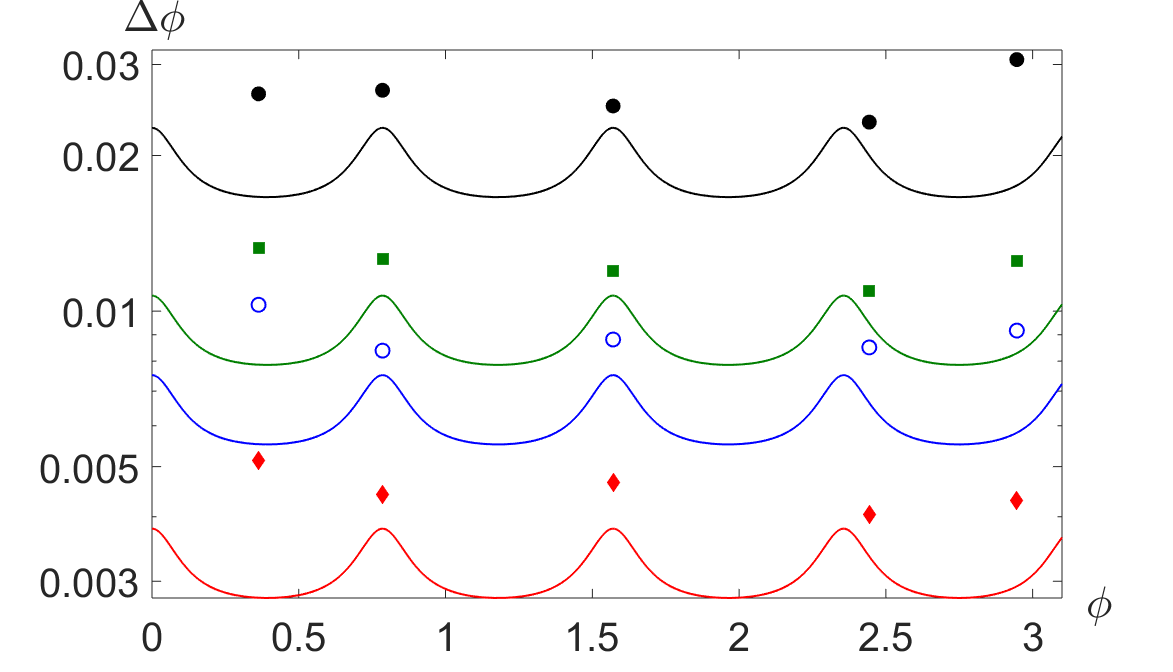 Figure 1
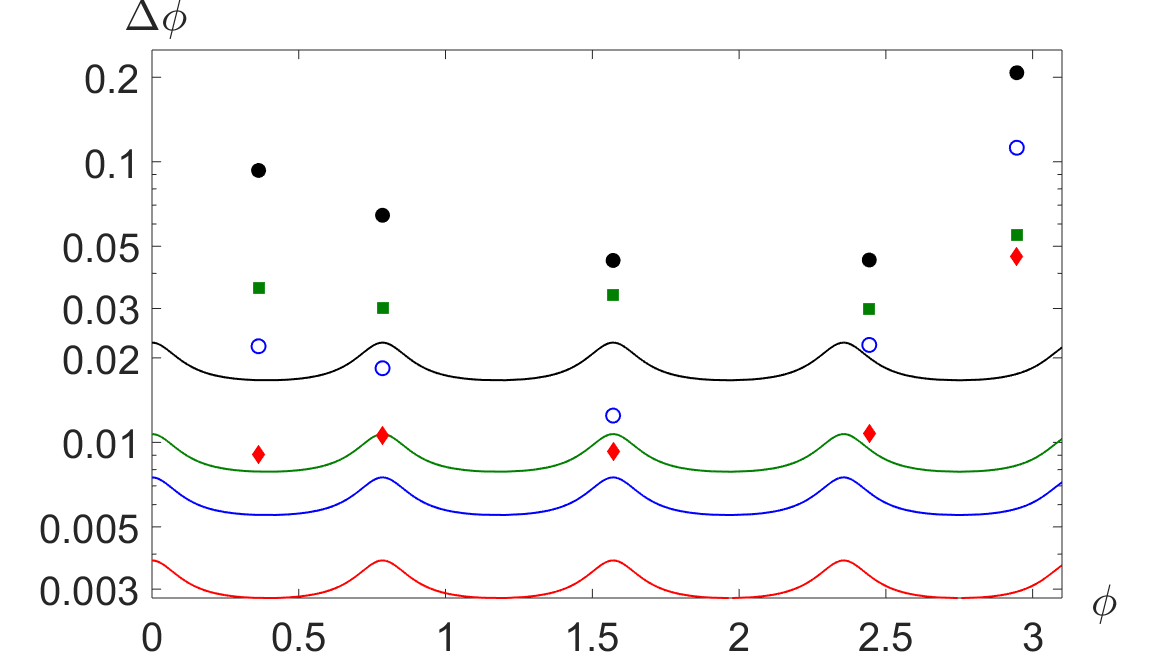 Figure 2
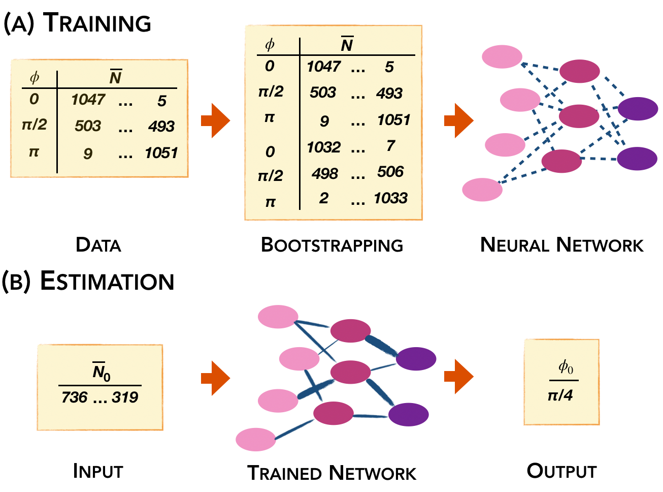 Figure 1
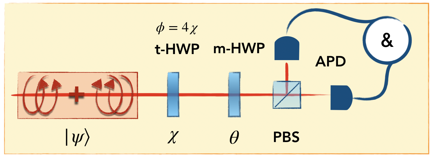 Figure 2
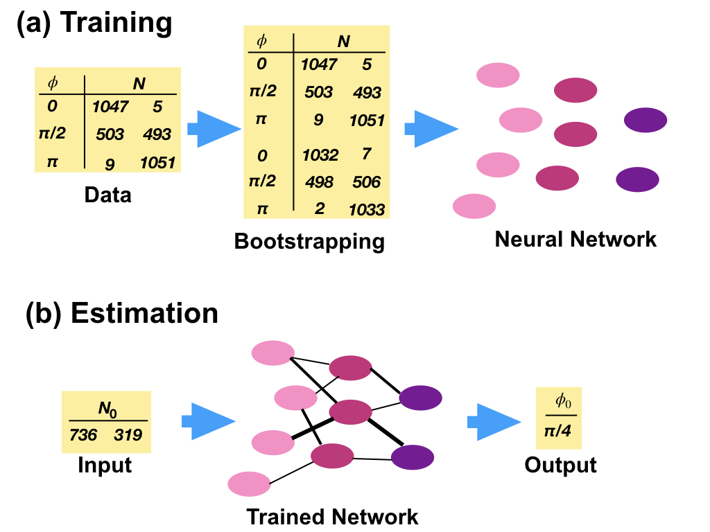 Figure 5
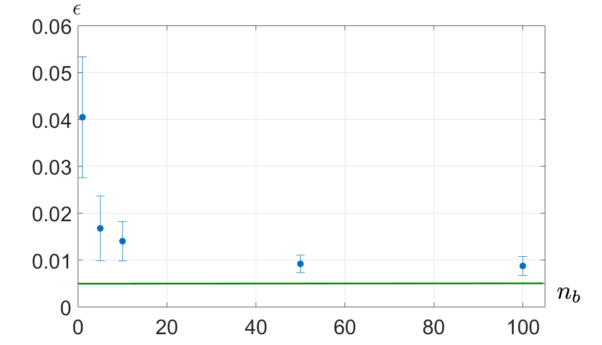 Figure 6
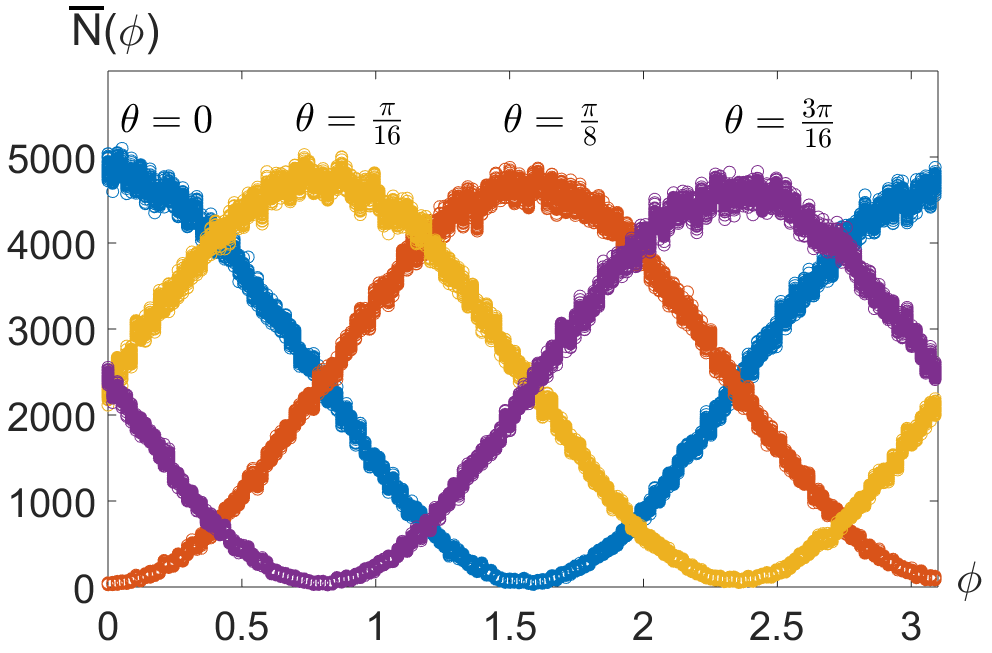 Figure 7
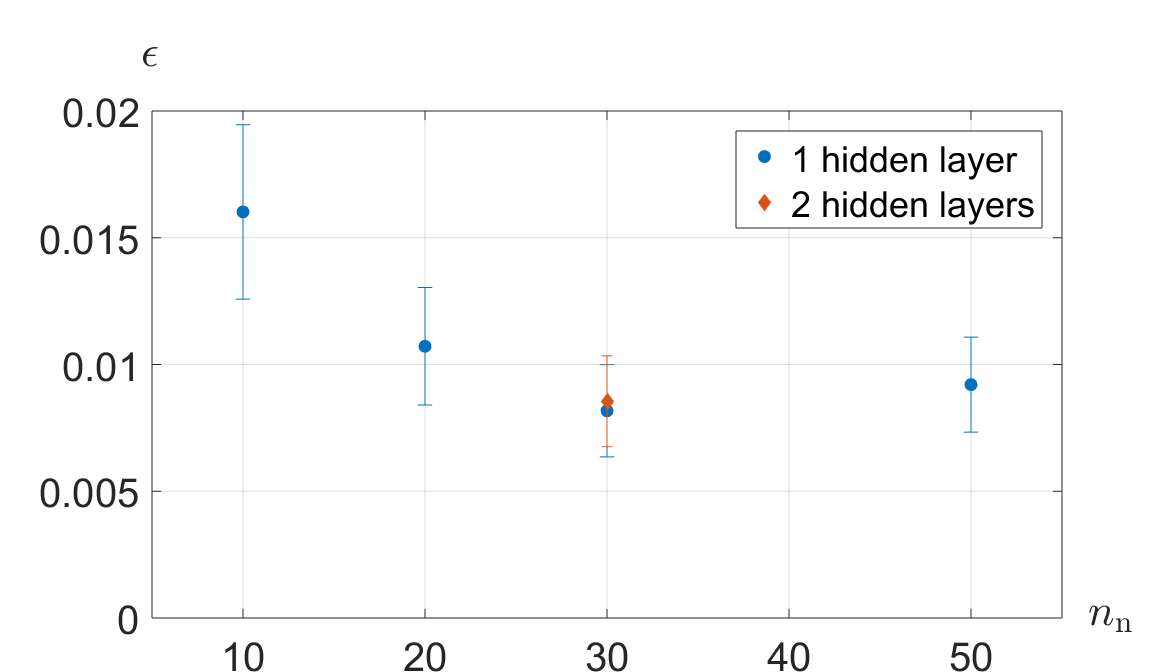 Figure 8
Peer Reviews
No public reviews on file for this paper yet. If you reviewed it on a platform where reviews are public (OpenReview, ICLR, NeurIPS, ICML), you can paste yours below so the community can read it here.
Videos
No videos yet. Explain this paper in a talk, walkthrough, or lecture? Add one.
Calibration of quantum sensors by neural networks
Valeria Cimini
Dipartimento di Scienze, Università degli Studi Roma Tre, Via della Vasca Navale 84, 00146, Rome, Italy
Ilaria Gianani
Dipartimento di Scienze, Università degli Studi Roma Tre, Via della Vasca Navale 84, 00146, Rome, Italy
Dipartimento di Fisica, Sapienza Università di Roma, P.le Aldo Moro, 5, 00185, Rome, Italy
Nicolò Spagnolo
Dipartimento di Fisica, Sapienza Università di Roma, P.le Aldo Moro, 5, 00185, Rome, Italy
Fabio Leccese
Dipartimento di Scienze, Università degli Studi Roma Tre, Via della Vasca Navale 84, 00146, Rome, Italy
Fabio Sciarrino
Dipartimento di Fisica, Sapienza Università di Roma, P.le Aldo Moro, 5, 00185, Rome, Italy
Marco Barbieri
Dipartimento di Scienze, Università degli Studi Roma Tre, Via della Vasca Navale 84, 00146, Rome, Italy
Istituto Nazionale di Ottica - CNR, Largo Enrico Fermi 6, 50125, Florence, Italy
Abstract
Introducing quantum sensors as solution to real-world problem demands reliability and controllability outside laboratory conditions. Producers and operators ought to be assumed to have limited resources ready available for calibration, and yet, they should be able to trust the devices. Neural networks are almost ubiquitous for similar tasks for classical sensors: here we show the applications of this technique to calibrating a quantum photonic sensor. This is based on a set of training data, collected only relying on the available probe states, hence reducing overheads. We found that covering finely the parameter space is key to achieve uncertainties close to their ultimate level. This technique has potential to become the standard approach to calibrate quantum sensors.
Quantum technologies are experiencing a world-wide effort to foster their applications beyond what is achieved in a laboratory. In particular for quantum sensing, quantum resources are promising to reach accuracy beyond what is permitted from classical counterparts Giovannetti et al. (2006). This advantage however, it is conditioned on a robust operation in the presence of noise as well as imperfections of the measuring instruments Dooley et al. (2018); Nichols et al. (2016). Many methods have been proposed to this end, including error correction Unden et al. (2016); Zhou et al. (2018); Reiter et al. (2017); Cohen et al. (2016), monitoring of the environment Albarelli et al. (2018), and imperfection-tollerant probe state design Kacprowicz et al. (2010); Thomas-Peter et al. (2011).
Regardless the method adopted, it is vital to devise analysis methods that grant optimal use of the collected data for estimation, i.e. to obtain the so called optimal estimator. For simple instances, the maximum likelihood approach or methods based on Bayes’ theorem are known to provide such an estimator Blandino et al. (2012); Lumino et al. (2018). On the other hand, these are generally computationally intensive, often require a more involved characterization of the system Lundeen et al. (2008); Zhang et al. (2012); Altorio et al. (2015); Roccia et al. (2018), and thus pose difficulties in scaling to configurations with increased complexity. Further, characterization is generally based on preparing quantum states with different requirements than those actually used in the estimation routine Brida et al. (2012); Rozema et al. (2014); Altorio et al. (2016). In the perspective of compact architectures, the resulting requirement of flexibility may come at odds with that of reliability and reduced costs Rudinger et al. (2017). A method being self-consistent, resource economic, and versatile is desirable.
Nowadays, the incredible amount of data collected in diverse problems requires efficient self-adjustment of the sorting protocol. The size and complexity of these problems has imposed Machine Learning (ML) algorithms as the mainstream solution in these situations Murphy (2012); Simon (2013). ML has been recently proposed and applied as tool for characterization and optimization of quantum systems as well as for handling quantum physics problems Dunjko and Briegel (2018). Notable examples include its adoption for the learnability of quantum measurements, states and processes Magesan et al. (2015); Aaronson (2007); Rocchetto et al. (2019); Yu et al. (2019); Spagnolo et al. (2017); Granade et al. (2012); Wang et al. (2017), validation of multiparticle interference Flamini et al. (2019); Agresti et al. (2019), quantum state engineering Innocenti et al. (2017); Giordani et al. (2019); Bukov et al. (2018), and as a tool for quantum experiment design and control Briegel and De las Cuevas (2012); Innocenti et al. ; Krenn et al. (2016); Melnikov et al. (2018); Las Heras et al. (2016); August and Ni (2017). In the context of quantum metrology, ML has found an application in quantum phase estimation protocols to efficiently extract the information encoded in the probe Wiebe et al. ; Wiebe and Granade (2016); Paesani et al. (2017). More specifically, ML represents a powerful toolbox to optimize, via adaptive protocols Hentschel and Sanders (2010, 2011); Lovett et al. (2013) the performance of a sensor operating with a small collection of repetitions Lumino et al. (2018). These considerations suggest the viability of this approach for a full characterization of quantum sensing apparata. Specifically, neural networks can extract an output value of the parameter of interest, following their training on a set of inputs associated to a calibrated set of parameters; this is an efficient algorithm that can be run on ordinary machines Caciotta et al. (2009, 2016). No explicit modelling of the imperfections is thus needed, as that information will be taken into account, although in implicit form, in the training itself. On the other hand, the training data can only be collected in finite time, hence with finest statistics: it is important to understand how the associated uncertainty influences the quality of the final estimation, and its capability of showing quantum enhancement.
In this article, we discuss the characterization of a quantum phase sensor based on N00N states by means of the neural network. We find that the simplicity of the characterisation does not impact heavily the metrological capabilities of the device. The algorithm has no strict requirements in its settings to provide near-optimal performance of the estimation, provided that the set of the parameter is explored with adequate resolution. Thanks to its compact implementation and its scalability, this method can find wide applications in future quantum technologies.
The concept behind our investigation is depicted in Fig. 1. The training step (Fig. 1a) consists in collecting a set of data corresponding to different values of the parameter of interest ; in general will be in the form of a vector, since it contains multiple measurements, as needed to obtain a correct normalization, to remove ambiguities, or to account for multiple parameters. This is used as an input to a network, consisting of a set of neurons connected among them, possibly forming subsequent layers. The training procedure establishes the weights associated to the connections between each pair of neurons. Unavoidably, an uncertainty will be associated to these measured data, and the network needs to be trained to account for this variability. If the noise statistics on each measurement in is known, a bootstrapping method can be employed to generate multiple fictitious runs of the experiment by means of a Monte Carlo routine. For a fixed network size, the quality of the training will be influenced by the resolution at which is sampled, as well as the number of repetitions of used for each value of . Once the training is complete, the device can be used for parameter estimation: the network is now operated to accept the collected data as an input, and to provide an estimation as the output (Fig. 1b). By using the same bootstrapping method above on , the uncertainty can also be evaluated.
We test this method in a quantum phase estimation experiment. A two-photon N00N state on the ight- and eft-circular polarisation of a single spatial mode approximating is used for this task (see Fig. 2). This is achieved by overlapping on the same spatial mode two otherwise-indistinguishable orthogonally polarized photons by means of a polarizing beam splitter (PBS) Slussarenko et al. (2017); Roccia et al. (2018): the photon pairs are generated via a type-I Spontaneous Parametric Down Conversion (SPDC) source using a 3mm BBO crystal pumped with a 405 nm CW laser; their polarization is then set orthogonal by means of Half Wave plates (HWPs) and they are sent on a PBS obtaining the circular polarization N00N state. The measurement is then carried out collecting a vector of coincidences counts associated to photon pairs after they have accumulated a relative phase , resulting from the rotation of their polarization state. For each phase, we look at the coincidences counts relative to four different polarizations projections Roccia et al. (2018).
Even in this simple instance, many imperfections affect the actual experimental apparatus including those linked to the phase preparation as well as imperfect splittings on the PBSs and polarization-dependent efficiencies of the detection channels. Scrupulous modelling should include several variables to account for these in a parameter-dependent way, making the problem involved. In more complex scenarios this becomes even more demanding. We test how the effectiveness of the implicit treatment of imperfections made possible by neural networks.
We collect data for different phase values from [math] to in steps of , simply obtained by rotating a half wave plate (HWP) from [math] to in steps of – the relation between the phase and the angle setting is . The initial training data thus consist of 180 vectors, each containing four counting rate. Each projection accumulated data for 1s, which, at the observed count rate, correspond to around 10000 total events for each phase, divided among the four projections (Fig. 2).
From all the coincidences counts we obtain the relative frequencies associated to that phase, and we use them for a supervised training of the network. In this way, we can use the network independently on the total number of collected events. Since these counts follow a Poissonian distribution, we can test the accuracy by using the bootstrap procedure described above to feed our network with different repetitions associated to each phase. The network is structured as a feed-forward network with sigmoid hidden neurons MathWorks (2019). This includes an input layer, and output layer, and a hidden layer with neurons. The input data are randomly divided in a training set (70%), a validation set (15%) and a test set (15%). The network is trained with Levenberg-Marquardt backpropagation algorithm designed to optimise for every phase, the precision on the validation set using the mean square error metric. The training stops when the validation error stops decreasing.
We have run tests on simulated data to establish the optimal parameters for the training for fixed sampling step and total count rate: for this purpose, we input in the trained network the counting rates corresponding to 30 values of the phase, and consider as the error the mean standard deviation calculated on 100 repetitions and averaged on all phases. Fig. 3 shows how this error depends on the number of neurons in the network, and on the number of Monte Carlo runs per phase value . The data do not show sharp optimal working points: we have adopted one hidden layer in the network with 30 neurons, trained with 50 Monte Carlo repetitions.
With the network settings so fixed, we have proceeded to feeding the actual data collected in the experiment for training. We have then collected 5 further sets for the phases 20.8∘, 45∘, 90∘, 140∘, and 168.8∘ at different accumulation times (0.5s, 1s, 4s) at the same generation rate as for the training, and 0.5s at 30% of the initial generation rate. These are used to observe how the uncertainty scales with the number of collected events . In Fig. 4, we show such uncertainties, compared to the associated Cramér-Rao bound (CRB) Giovannetti et al. (2006); Paris (2009). The uncertainties remain close to the ultimate limit which also takes into account the reduced contrast of the coincidence oscillations. Remarkably, we observe an improvement also for number of events exceeding those used for the training. The employ of the neural network makes this characterisation robust to noise. We have repeated the training stage decreasing the step size of the phase to . The distance to the CRB is more pronounced: the network has received insufficient training to produce an output with an accuracy close to optimal. We noticed that, also in this case, a reduction of the uncertainty is observed when increasing the number of events . We put these observations in quantitative terms by inspecting , i.e the ratio between the measured variance and the one at the CRB at a given . We obtain the following values: , , , . We note that the F value increases with the repetition number, which implies that variance is diminishing with M however not as fast as the CRB is. This is due to the lack of resolution in the training, which is not a fundamental limit, and in our case it is solely constrained by the accuracy of the actuator of m-HWP.
While overall successful, this characterization underlines some issues which need to be addressed. Close to and , a boundary effect can be observed that prevents from obtaining a reliable estimate close to this value; this is removed by increasing the region explored for the training, which should span a wider interval than the one potentially covered in the measurement. Excess uncertainty is associated to phases close to , a problem we can attribute to the particular symmetries of the count signals (see Fig. 2). We further note that using these four count signals allows to suppress the periodicity ambiguity on the phase in the range 0 - , but still leaves an ambiguity in the range 0 - . This latter ambiguity can be approached by integrating adaptive techniques Lumino et al. (2018) within the phase estimation protocol.
In conclusion, we have applied a neural network algorithm to the calibration of a quantum phase sensor. This method compares favourably to previous investigations that require a complete reconstruction of the functioning of the device Lundeen et al. (2008); Zhang et al. (2012) or to the data fitting pattern technique Altorio et al. (2016). The advantage stems on the one hand from the more efficient data processing, and from the resilience to noise that overcomes the need for regularisation of the data. On the other hand, the characterisation can be carried out only by means of the same kind of states employed in the actual measurement. This is particularly relevant in the perspective of large-scale fabrication of such devices, for which an analysis based on off-line characterisation states would be impractical.
This advantage is kept also with respect to cases in which an effective characterisation can be carried out in terms of extra parameters – as long these remain fixed. Indeed, this would rely on a modelling of the imperfections, that might only be captured in part.
Further perspectives of this work can be found in extending the application of neural networks for the calibration of quantum sensors operating in the multiparameter regime, where multiple phases Humphreys et al. (2013); Ciampini et al. (2016); Pezzè et al. (2017); Polino et al. (2019) and relevant system physical quantities Roccia et al. (2018); Cimini et al. , including noise, have to measured simultaneously. Indeed, in those scenario reliable calibration methods becomes particularly crucial due to the increasing complexity of characterising all the system parameters, as well as the computational overhead in handling large amount of data.
Note added. - During the completion of this manuscript, we became aware of two works Macarone-Palmier et al. ; Torlai et al. , where neural networks have been applied to quantum state estimation and quantum simulation.
Acknowledgements.
We acknowledge support from the Amaldi Research Center funded by the MIUR program ”Dipartimento di Eccellenza” (CUP:B81I18001170001).
The reference list from the paper itself. Each links out to its DOI / PubMed record.
- 1Giovannetti et al. (2006) V. Giovannetti, S. Lloyd, and L. Maccone, Phys. Rev. Lett. 96 , 010401 (2006) . · doi ↗
- 2Dooley et al. (2018) S. Dooley, M. Hanks, S. Nakayama, W. J. Munro, and K. Nemoto, npj Quantum Information 4 , 24 (2018) . · doi ↗
- 3Nichols et al. (2016) R. Nichols, T. R. Bromley, L. A. Correa, and G. Adesso, Phys. Rev. A 94 , 042101 (2016) . · doi ↗
- 4Unden et al. (2016) T. Unden, P. Balasubramanian, D. Louzon, Y. Vinkler, M. B. Plenio, M. Markham, D. Twitchen, A. Stacey, I. Lovchinsky, A. O. Sushkov, M. D. Lukin, A. Retzker, B. Naydenov, L. P. Mc Guinness, and F. Jelezko, Phys. Rev. Lett. 116 , 230502 (2016) . · doi ↗
- 5Zhou et al. (2018) S. Zhou, M. Zhang, J. Preskill, and L. Jiang, Nature Communications 9 , 78 (2018) . · doi ↗
- 6Reiter et al. (2017) F. Reiter, A. S. Sørensen, P. Zoller, and C. A. Muschik, Nature Communications 8 , 1822 (2017) . · doi ↗
- 7Cohen et al. (2016) L. Cohen, Y. Pilnyak, D. Istrati, A. Retzker, and H. S. Eisenberg, Phys. Rev. A 94 , 012324 (2016) . · doi ↗
- 8Albarelli et al. (2018) F. Albarelli, M. A. C. Rossi, D. Tamascelli, and M. G. Genoni, Quantum 2 , 110 (2018).