Thermodynamic constraints on matter creation models
R. Valentim, J. F. Jesus

TL;DR
This paper uses thermodynamic principles, particularly entropy conditions, to analyze and constrain matter creation models in cosmology, focusing on the evolution of entropy across different eras of the universe.
Contribution
It introduces a thermodynamic framework based on entropy derivatives to estimate parameter intervals in Creation Cold Dark Matter models.
Findings
Entropy conditions restrict model parameters.
Thermodynamic equilibrium is achieved in a final de Sitter era.
Total entropy includes horizon, matter, and radiation contributions.
Abstract
Entropy is a fundamental concept from Thermodynamics and it can be used to study models on context of Creation Cold Dark Matter (CCDM). From conditions on the first ()\footnote{Throughout the present work we will use dots to indicate time derivatives and dashes to indicate derivatives with respect to scale factor.} and second order () time derivatives of total entropy in the initial expansion of Sitter through the radiation and matter eras until the end of Sitter expansion, it is possible to estimate the intervals of parameters. The total entropy () is calculated as sum of the entropy at all eras ( and ) plus the entropy of the event horizon (). This term derives from the Holographic Principle where it suggests that all information is contained on the observable horizon. The main feature of this method for these models are that…
Click any figure to enlarge with its caption.
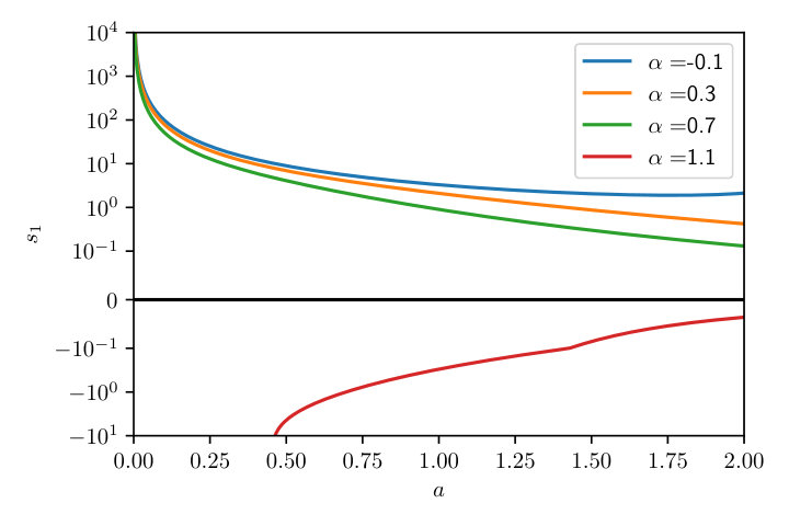 Figure 1
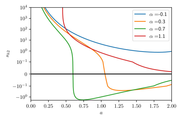 Figure 2
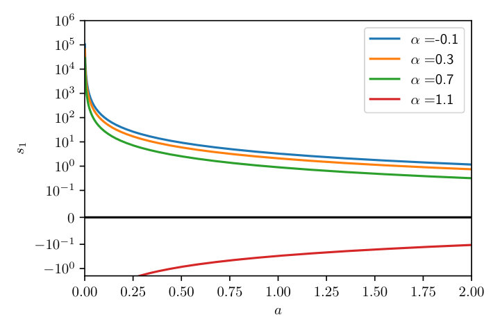 Figure 3
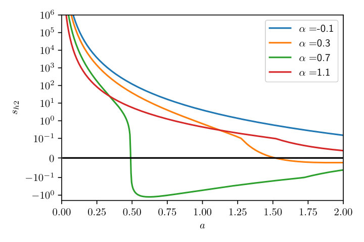 Figure 4
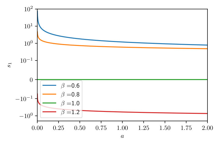 Figure 5
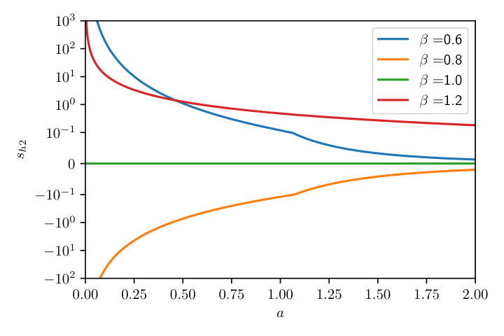 Figure 6
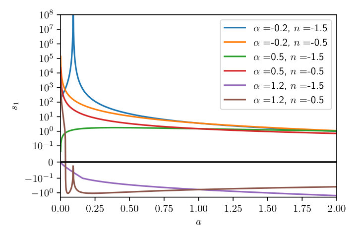 Figure 7
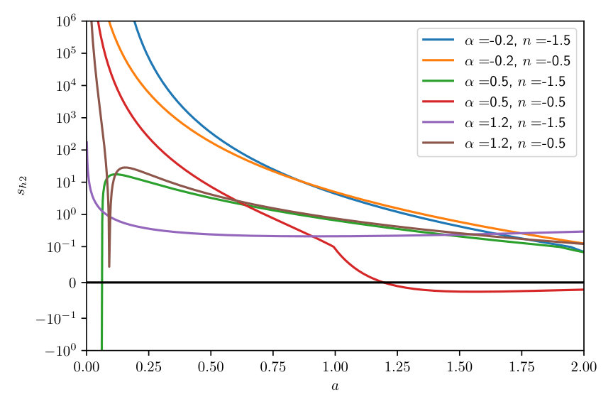 Figure 8
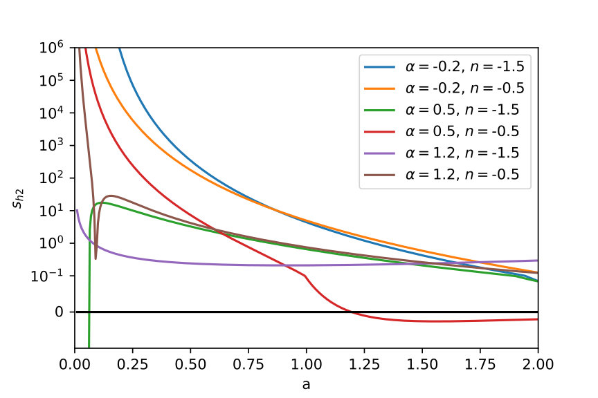 Figure 9
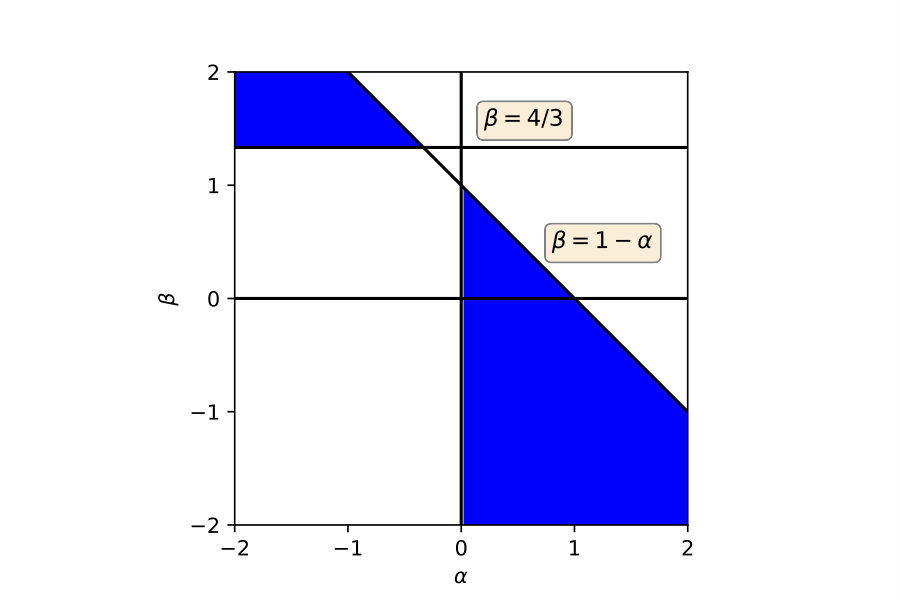 Figure 10
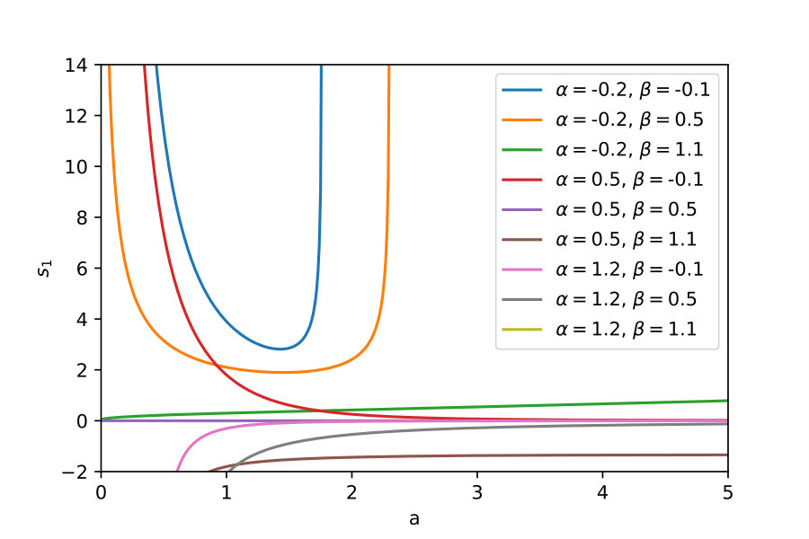 Figure 11
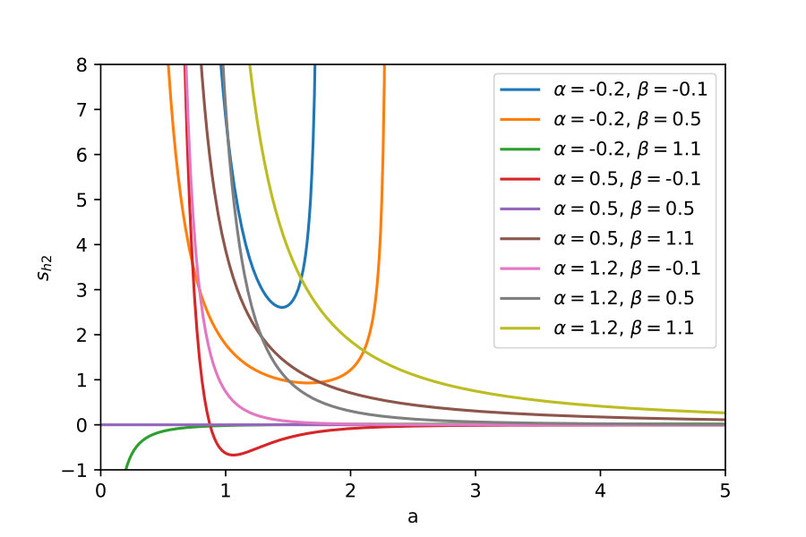 Figure 12
| Model | Creation rate | Reference | Parameters |
|---|---|---|---|
| JO16 (JO) | , | ||
| GraefEtAl14 | , | ||
| – | |||
| – | |||
| GraefEtAl14 |
| Model | Creation rate | Combination | |||
|---|---|---|---|---|---|
| , | , | , | |||
| , |
Peer Reviews
No public reviews on file for this paper yet. If you reviewed it on a platform where reviews are public (OpenReview, ICLR, NeurIPS, ICML), you can paste yours below so the community can read it here.
Videos
No videos yet. Explain this paper in a talk, walkthrough, or lecture? Add one.
Thermodynamic constraints on matter creation models
R. Valentim
Departamento de Física, Instituto de Ciências Ambientais, Químicas e Farmacêuticas - ICAQF, Universidade Federal de São Paulo (UNIFESP) Unidade José Alencar, Rua São Nicolau No. 210, 09913-030 – Diadema, SP, Brazil
J. F. Jesus
Universidade Estadual Paulista (UNESP), Câmpus Experimental de Itapeva
Rua Geraldo Alckmin 519, 18409-010, Vila N. Sra. de Fátima, Itapeva, SP, Brazil
Universidade Estadual Paulista (UNESP), Faculdade de Engenharia de Guaratinguetá
Departamento de Física e Química, Av. Dr. Ariberto Pereira da Cunha 333, 12516-410 - Guaratinguetá, SP, Brazil
Abstract
Entropy is a fundamental concept from Thermodynamics and it can be used to study models on context of Creation Cold Dark Matter (CCDM). From conditions on the first ()111Throughout the present work we will use dots to indicate time derivatives and dashes to indicate derivatives with respect to scale factor. and second order () time derivatives of total entropy in the initial expansion of Sitter through the radiation and matter eras until the end of Sitter expansion, it is possible to estimate the intervals of parameters. The total entropy () is calculated as sum of the entropy at all eras ( and ) plus the entropy of the event horizon (). This term derives from the Holographic Principle where it suggests that all information is contained on the observable horizon. The main feature of this method for these models are that thermodynamic equilibrium is reached in a final de Sitter era. Total entropy of the universe is calculated with three terms: apparent horizon (), entropy of matter () and entropy of radiation (). This analysis allows to estimate intervals of parameters of CCDM models.
Entropy, Holographic Principle and CCDM models
I Introduction
When physical systems are isolated they tend spontaneously to reach thermodynamic equilibrium. This idea is at the empirical basis of the Second Law of Thermodynamics: that the entropy () for closed systems remain constant or increase with time (). The second order entropy derivative with respect to the relevant variable must obey , at least roughly, when the Universe keeps to expand on the infinite future. It leads to thermodynamic equilibrium Callen1985 ; MimosoPavon2013 . One way of assuming the condition on second order derivatives in cosmic expansion is through the Holographic Principle proposed by t'Hooft1993 ; Susskind1995 that was directly applied in Cosmology FischlerSusskind1998 ; BakRey2000 . This principle assumes that all information is on the Universe horizon surface.
The matter creation in the context of cosmology has been studied by different authors. Ref. Parker1968 investigated particle creation mechanisms using covariant quantized free field equations of elementary particles in the expansion of the Universe. In this work, the author analysed the creation of particles with spin–0 pions, spin–1/2 and particles with zero mass and non-zero rotation.
Prigogine et al. PrigogineEtAl1988 argue that Einstein’s equations for General Relativity are adiabatic and reversible, so they do not allow the production of entropy in a cosmological scenario. The authors proposed a way to solve this problem based on the idea of irreversibility of thermodynamic systems. Authors showed that the Thermodynamics of irreversible systems leads naturally to a reinterpretation of Einstein’s equations, which allows the creation of matter from the gravitational field and consequently the production of entropy. The cosmological history proposed by PrigogineEtAl1988 has three stages: first, from an initial vacuum fluctuation in de Sitter’s space; second, that de Sitter space exists during a time of decay of its constituents; third, a phase transition transforms this de Sitter space into a universe with a Friedman-Robertson-Walker metric that evolves adiabatically on the cosmological scale. An important aspect to be emphasized is that the approach of the matter creation does not consider Dark Matter and Dark Energy scenarios. A natural consequence of this approach is the rate of change in the number of particles, , which spells out the Second Law of Thermodynamics. There are still unanswered questions about the creation mechanism () from the gravitational field, the physical nature of the particles and how influences the expansion of the universe PanEtAl2016 . Some authors suggest that the type of particles created in this process are limited by local links related to gravity EllisEtAl1989 ; HagiwaraEtAl2002 ; PeeblesRatra2003 . These authors showed that radiation does not contribute significantly to the late accelerated expansion of the universe in the dominant dark matter phase. Some later work suggests that the particles produced by the gravitational field are Cold Dark Matter (CDM) particles and that for the rates of matter creation () may constrain CDM SteigmanEtAl2009 ; LimaEtAl2010 ; FabrisEtAl2014 ; LimaEtAl2014 ; ChakrabortyEtAl2015 .
In a recent work NunesPavon2015 , the authors present the possibility of a quantum vacuum equation of state associated with the creation of particles by the gravitational field that acts in a vacuum. They analyzed three different matter creation rates and estimated the parameters from SNe Ia, Gamma Ray Bursts (GRBs), Baryon Acoustic Oscillations (BAO) and Hubble parameter data. The authors show that matter creation models can explain the phantom behaviour of our Universe without the need to insert phantom fields Cadwell2002 . The work proposed by PanEtAl2016 analyses how the process of matter creation happens with the universe expanding. In the context analysed by the authors, the gravitational field induces a process of adiabatic matter creation. In this work, PanEtAl2016 present a generalized model for with three free parameters PanChakraborty2015 ; ChakrabortyEtAl2014 . This model encompasses the transition from the inflationary phase to the radiation phase for adiabatic particle production. In another recent work PanEtAl2019 , it is proposed a two-fluid model where one fluid () is produced adiabatically and there is another fluid that does not interact with fluid 1 and satisfies the energy conservation equation. One important aspect of the work is the study of the singularities of from the analysis of a series expansion. With this they plot the profiles of according to the scale parameter () for each in relation to the terms of the expansion of . Although interesting the idea of a series expansion, we shall restrict ourselves here to the analysis of a simpler and yet broad class of matter creation models.
We will explore in this work the calculations of the total entropy () from the holographic principle for five models of matter creation. These models were studied by bic-ccdm and it assumes that the creation rate is a function of the Hubble parameter . Each dark matter creation rate leads to a different cosmic evolution GraefEtAl2014 ; Freaza2002 ; Lima2008 ; JO16 ; Lima2010 ; LimaBasilakos2012 ; LimaBasilakos2013 222See also JesusPereira14 ; LimaBaranov14 for more fundamental formulations of matter creation models.. A common feature of these models is that the Universe starts in an inflationary, de Sitter phase, then it passes through the ages of radiation and matter, where it finally enters the final de Sitter stage. Total entropy () at each phase is equal to the sum of each entropy contribution for these different ages. is the direct sum of the contribution of entropy to radiation, matter and the apparent horizon of the Holographic Principle t'Hooft1993 ; Susskind1995 :
[TABLE]
where , is the entropy of the apparent horizon, is entropy of pressureless matter and is entropy of radiation. and denote the area of the horizon and Planck’s length, respectively. In an ever expanding Universe, the conditions , are equivalent to the conditions , . Restricting our analysis to this class of models, we shall consider the entropy as a function of the scale factor from now on.
In this work, entropy evolution will be considered, initially based on the model proposed by LimaBasilakos2012 ; LimaBasilakos2013 and the models analyzed by bic-ccdm . We can use the conditions on the derivatives of the total entropy to estimate the intervals of validity of free parameters for each model MimosoPavon2013 . We shall assume a FRW metric, in agreement with the Cosmological Principle, and a spatially flat universe, as predicted from most inflationary models. However, recently, Ref. DiValentino2019 have shown from Planck Legacy 2018 dataset analysis that the curvature parameter can have a non-zero value, namely, at 99% c.l. As this “new” value of is a controversial theme, and the deviation from spatial flatness seems to be small, we prefer to use the standard value in this work, as predicted by most inflationary models. So, we are restricting our analysis to spatially flat models ().
II Creation of Cold Dark Matter Models (CCDM)
Models of CCDM used in this work it were statistically analyzed by bic-ccdm and have a natural dependence of (), where as function of Hubble parameter represents a relation between the matter creation and expansion rates. All the CCDM models used here have also free parameters. The models studied here were analyzed by bic-ccdm using three statistical criteria: Bayesian Information Criterion (BIC), Akaike Information Criterion (AIC) and Bayesian Evidence (BE) using the SNe Ia dataset. Most of these models can be described by a function , where and . So, it corresponds to a creation rate .
Another model analyzed in bic-ccdm is LJO ljo10 with . The LJO model has the same dynamics as concordance model. In LJO, the cosmological constant is exactly mimicked by particle creation. Due to this mimicking, we choose not to analyze this model here, as CDM has already been thoroughly analyzed on RadPav12 . In all models analyzed in this work we have neglected the contribution of baryons. The baryonic contribution is small, of Universe content and our results can be more dependent on the assumptions made here in order to estimate entropy rather than baryonic influence. Another important assumption is that Universe is spatially flat as indicated from CMB and preferred by inflation, i.e. in our analysis. The models studies here are described on Table 1.
III Methodology
The methodology adopted here consists on analyzing total entropy of the Universe in the context of matter creation models. This analysis allows to estimate the validity interval for free parameters for each model. This idea is based on MimosoPavon2013 , where authors analyzed first and second order derivatives. It assumes the Second Law of Thermodynamics jointly with the idea that thermodynamic equilibrium must be achieved at some future time. An important aspect of this method is that it takes into account the horizon entropy that came from Holographic Principle t'Hooft1993 ; Susskind1995 ; FischlerSusskind1998 where all the information about Universe is on horizon. The total entropy is given by equation (1) and it is defined as sum of radiation, matter and apparent horizon. Restricting our analysis to CCDM models Calvao1992 ; Lima2012 ; LimaBasilakos2013 ; bic-ccdm ; GraefEtAl14 , entropy was considered as a function of the scale factor. In CCDM, expansion acceleration can be achieved through an effective creation pressure:
[TABLE]
where is creation pressure, is dark matter (DM) density (pressure vanishes for DM), is creation rate and is Hubble parameter. Relation between Hubble parameter and is the Friedmann equation:
[TABLE]
for spatially flat Universe (). The equation of continuity for dark matter now reads:
[TABLE]
That is is a source () or sink () for dark matter. The Hubble parameter corresponds to the expansion rate, that is, , so, writing it as a function of scale factor, we have:
[TABLE]
where we denoted the derivative with respect to with a prime. The relation between matter density and particle number density is , where is mass of DM particle, so, we have:
[TABLE]
The Friedmann equation and continuity equation fully describe the CCDM background dynamics. From these equations we can derive a relation between and :
[TABLE]
or, in terms of scale factor,
[TABLE]
This class of models suggests that matter creation () generates a negative pressure () which may explain the acceleration of the Universe.
IV Thermodynamics of Matter Creation Models
In our analysis we are interested only on recent and future times, so we shall restrict ourselves to the matter dominated age, as radiation becomes negligible in the past. From equation (1), shown earlier, we will analyze the derivatives of each of the terms for the total entropy: entropy of the apparent horizon, matter and radiation MimosoPavon2013 .
Entropy of apparent horizon is , where denotes the area of apparent horizon and is Planck’s length. The area of the apparent horizon is given by , where . As explained above, we are restricting our analysis to spatially flat models (). This assumption yields and . In this case, the horizon entropy reads:
[TABLE]
That is, the entropy is function of Hubble parameter only. Thus, the first derivative of apparent horizon entropy with respect to scale factor is:
[TABLE]
The first-order derivative of the entropy results in an expression that is a function of and its first derivative. Eq. (8) yields , thus we may write for :
[TABLE]
For the entropy, we may consider that every single particle contributes to the entropy inside the horizon by a single bit, MimosoPavon2013 . In this case, we have:
[TABLE]
where is the number density. By deriving this equation we find:
[TABLE]
This expression is first derivative of entropy as function of , and . By using Eqs. (6) and (8), we may write:
[TABLE]
That is, the derivative of entropy of matter as function of , and . Now combining Eqs. (10) and (14), we have
[TABLE]
So, a necessary and sufficient condition for having is , that is, the particle creation rate must be less or equal to the volumetric expansion rate333Any volume in the Hubble flow scales with , thus .. Let us define the dimensionless quantity :
[TABLE]
Thus, corresponds to . Now, let us impose the concavity condition , that is, impose that the Universe reaches thermodynamic equilibrium in the infinite future. By deriving (10):
[TABLE]
Using and deriving the Friedmann equation (3), we have
[TABLE]
Combining this with the Friedmann equation, we find the relation444It can also be found from Eqs. (6) and (8).
[TABLE]
That is, the particle density relative variation (w.r.t. ) is double of Hubble parameter relative variation. We may use this to simplify Eq. (13):
[TABLE]
Now it is easier to derive it to find :
[TABLE]
where we have derived (20) and used the relation (19) again in order to omit derivatives. By summing (17) and (21), we find:
[TABLE]
Let us define the dimensionless quantities:
[TABLE]
Thus, the conditions and correspond to and , respectively. A sufficient (but not necessary) condition for having is having both and . Although it may be too restrictive a condition over the models, we consider it reasonable in order to achieve a result not much dependent on the choice of the contribution of each particle to the entropy ().
Another interesting inference we can make from expressions (23) and (24) is that , so at all times, so every time that , we have . That is, implies .
In the next section we will analyze a quite general model for the rate of creation of dark matter with three free parameters.
V Case Study:
We now analyze a quite general model of the matter creation rate which was derived by GraefEtAl14 with three free parameters: , and . All the models that we will deal with here are particular cases of this model whose dependence with is given by:
[TABLE]
This model for is a combination of two important dependencies: the first term and the second term . In this case, Eq. (8) reads
[TABLE]
where . As shown by bic-ccdm , Eq. (26) can be solved as
[TABLE]
in case that and . Case is equivalent to . If , can be obtained from (26) as
[TABLE]
The eq. (27) shows as a function of scale factor , , , and . By writing as an explicit function of the parameters, we can now impose the condition . From the Eq. (15) and (16) it yields:
[TABLE]
We must have at all times, so we must have by this analysis.
According to (17), implies , so
[TABLE]
Now, let us impose the condition . It implies, from (21) that . We have
[TABLE]
We remind that we are interested in the sign of (30) and (31) only in the limit . However, this limit is strongly dependent in the parameter set , so, instead of putting limits for the general model, we shall put limits for each particular model. Let us do it in next subsections.
V.1
In this case we have the fixed parameter values and , so from (29) we see that reads
[TABLE]
which implies . From (30), the condition reads
[TABLE]
Thus, for , it implies . From (31), the condition reads
[TABLE]
which yields the same limit for , .
In Figure 1, we may see that for and for , in agreement with our analysis. As discussed above, implies , so we choose to plot only and for each model, for clarity.
V.2
In this case we have the fixed parameter values and , so from (29) we see that reads
[TABLE]
which implies . From (30), the condition reads
[TABLE]
Thus, for , it implies . From (31), the condition reads
[TABLE]
which yields the same limit for , .
In Figure 2, we may see that for and for , in agreement with our analysis.
V.3 :
In this case we have the fixed parameter value , so from (29) we see that reads
[TABLE]
which implies . From (30), the condition reads
[TABLE]
Thus, it implies . From (31), the condition reads
[TABLE]
which yields the limit . As one may see, for all the interval that we have we have also , as expected.
In Figure 3, we may see that for and for , in agreement with our analysis.
V.4
In this case we have the fixed parameter value , so from (29) we see that reads
[TABLE]
which implies . From (30), the condition reads
[TABLE]
For , there are some subcases here, according to the sign of the exponent , that is, if is greater than or not. If , the condition can be summarized as . As , it implies . If , the condition is , which is impossible, so is discarded by this analysis. In the special case of , we recover the model , so .
From (31), the condition reads
[TABLE]
which yields the same limit for and : . Just like before, implies, like in , .
In Figure 4, we may see that for and for and , in agreement with our analysis.
V.5
In this case we have the fixed parameter value , so from (29) we see that reads
[TABLE]
which implies . From (30), the condition reads
[TABLE]
To analyze the behaviour for we have to make assumptions about the scale factor exponent, . If , implies . If we combine with the condition from , we must have , thus it simplifies to . Thus, and or and .
For , would imply , so is not allowed by this analysis.
If , Eq. (28) with yields
[TABLE]
from which we find
[TABLE]
In this case, in the limit , implies , that is, is not allowed by this analysis.
From (31), the condition reads
[TABLE]
In this case, in the limit , for , implies . Combining it with the condition from , we have , thus . So, if , and if , we have .
For , would imply , so is not allowed by this analysis.
For , is written:
[TABLE]
In this case, in the limit , implies , that is, is not allowed by this analysis. The limits for model can be viewed on Fig. 5.
In Figure 6, we may see that for and for and , in agreement with our analysis.
The results of all models from Table 1 can be seen on Table 2.
VI Discussion and Concluding Remarks
We have analyzed the thermodynamics of 5 spatially flat CCDM models, taking into account a contribution from the horizon entropy, based on Holographic Principle.
In principle, the initial state of de Sitter age should be stable ( and constants when ) but particle creation (), according to MimosoPavon2013 , can be seen as an external agent acting on the system. Before the thermodynamic equilibrium was reached, the Universe needed to self-adjust to allow the ultimate expansion of de Sitter through the ages of radiation and matter.
The rate of particle production is irreversible, in this case for the five models treated in this work. In practice, irreversibility directly implies the generation of entropy Calvao1992 , as well as the increase in volume in the phase space. In our analysis, the particle production rate for the five models analyzed, was implicitly or explicitly included in the expressions for and , as can be seen in equations (15) and (22). For easy of analysis we defined the quantities for the first derivative and and for the second order derivatives. All models discussed in this work are particular cases of the general model with three free parameters: , and . The model has only one free parameter and the analysis of the derivatives suggests that it is between . is a model similar to but with constant , the limits for is . The model has as a free parameter and varies linearly with and . has two free parameters: and , is a power law over : . The validity interval was with , for corresponds to and if it becomes . For the model , which is a combination of and , and .
The limits over the parameters and could be seen in figure 5.
It is also interesting to mention that some of the models analyzed here can lead to singularities in the future () and to see how it compares with the thermodynamic constraints we found. Models – give no singularity at the future. Models and yield future singularities for some regions of the parameters. Model will have future singularity for and or and . It is important to notice that this region is disallowed from our thermodynamic analysis. Model will have future singularity for and or and . For this model, the thermodynamic analysis allows a future singularity only for and . Concerning our thermodynamic analysis, we found no problem with this region of the parameter space.
Further analysis of matter creation models may include the conserved baryonic contribution and spatial curvature. It could be interesting to test if the baryonic contribution, although small, could give non-negligible changes to the constraints we found. It is also interesting to see if this thermodynamic analysis could contribute to the current tension of constraints over the spatial curvature DiValentino2019 . Other creation rates not considered here could also be analyzed.
Acknowledgements.
JFJ has been supported by Fundação de Amparo à Pesquisa do Estado de São Paulo - FAPESP (Process no. 2017/05859-0) and R. V. has been supported by Fundação de Amparo à Pesquisa do Estado de São Paulo - FAPESP (Process no. 2013/26258-4 and 2016/09831-0). This study was financed in part by the Coordenação de Aperfeiçoamento de Pessoal de Nível Superior - Brasil (CAPES) - Finance Code 001.
The reference list from the paper itself. Each links out to its DOI / PubMed record.
- 1(1) H. B. Callen, “Thermodynamics and an Introduction to Thermostatistics”, 2nd Edition, pp. 512. Wiley-VCH,1985.
- 2(2) J. P. Mimoso & D. Pavón, Phys. Rev. D, 87, 047302, 2013.
- 3(3) G. ’t Hooft, 1993, ar Xiv:gr-qc/9310026.
- 4(4) L. Susskind, Journal of Mathematical Physics, 36, 6377, 1995.
- 5(5) W. Fischler & L. Susskind, ar Xiv:hep-th/9806039, 1998.
- 6(6) D. Bak & S. J. Rey, Classical and Quantum Gravity, 17, L 83, 2000.
- 7(7) L. Parker, Phys. Rev. Letters, vol. 21 , 8, pp. 562-564, 1968.
- 8(8) I. Prigogine, J. Geheniau, E. Gunzig, P. Nardone, 1989, Gen. Relativ. Grav., 21, 767, 1989.