TL;DR
This paper introduces Perturbed Amplitude Flow (PAF), a simple, efficient non-convex algorithm for phase retrieval that guarantees linear convergence with optimal measurements and is validated through simulations and image experiments.
Contribution
The paper presents PAF, a novel non-convex phase retrieval algorithm with proven recovery guarantees and linear convergence, requiring no truncation or re-weighting.
Findings
PAF recovers signals with optimal O(n) measurements.
PAF converges linearly from a designed initial point.
Validated effectiveness through simulations and natural image experiments.
Abstract
In this paper, we propose a new non-convex algorithm for solving the phase retrieval problem, i.e., the reconstruction of a signal \vx\in\H^n ( or ) from phaseless samples , . The proposed algorithm solves a new proposed model, perturbed amplitude-based model, for phase retrieval and is correspondingly named as {\em Perturbed Amplitude Flow} (PAF). We prove that PAF can recover () under Gaussian random measurements (optimal order of measurements). Starting with a designed initial point, our PAF algorithm iteratively converges to the true solution at a linear rate for both real and complex signals. Besides, PAF algorithm needn't any truncation or re-weighted procedure, so it enjoys simplicity for implementation. The effectiveness and benefit of the proposed method are validated by…
Click any figure to enlarge with its caption.
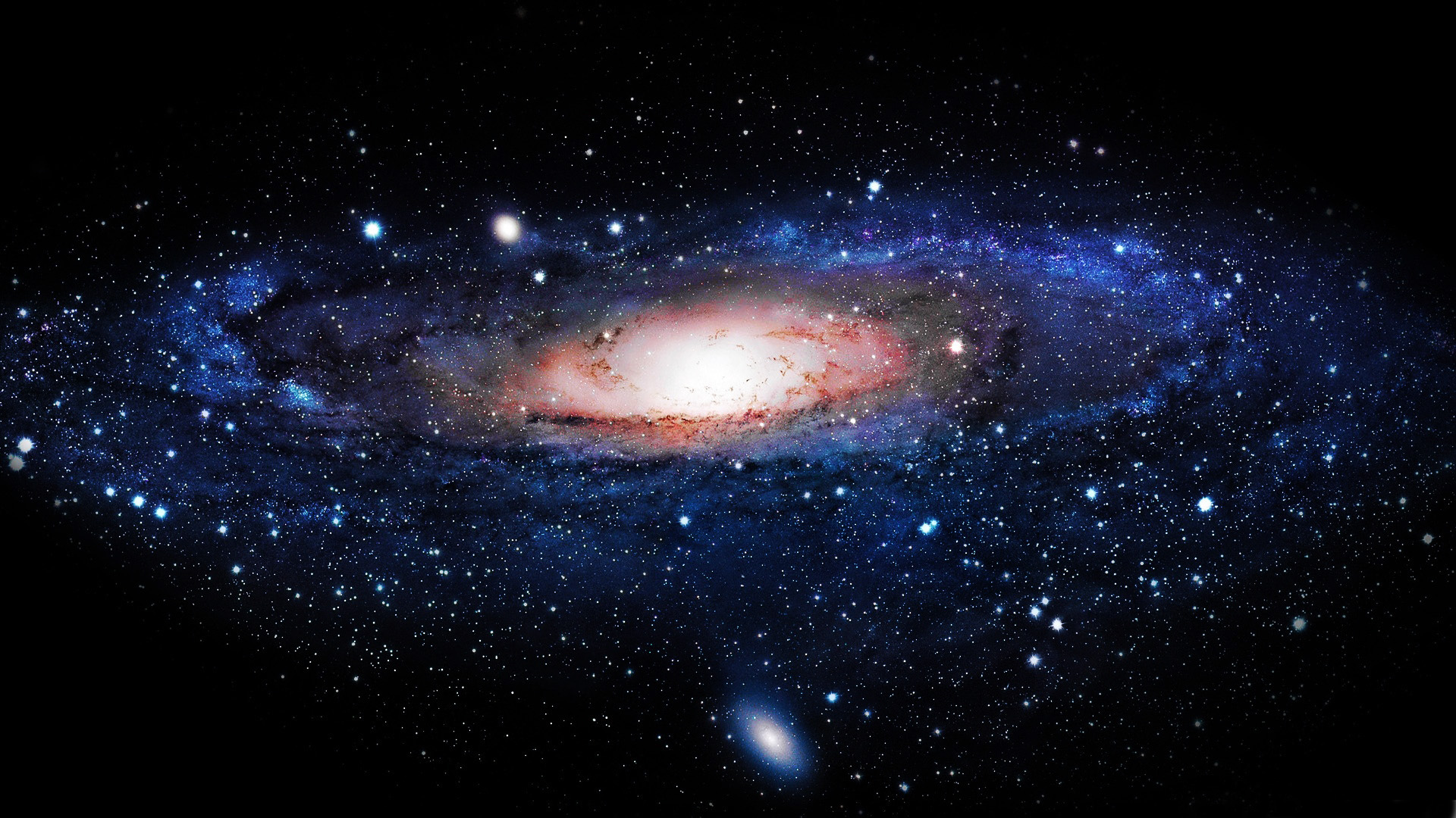 Figure 1
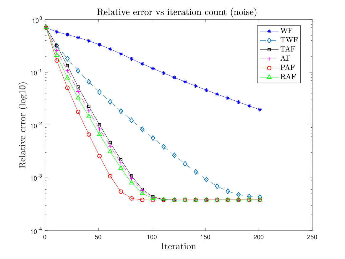 Figure 2
 Figure 3
 Figure 4
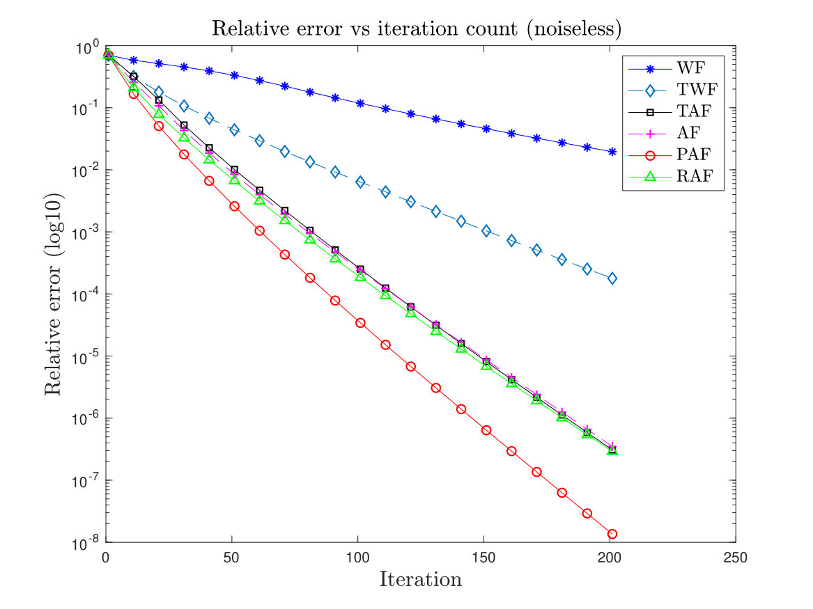 Figure 5
 Figure 6
 Figure 7
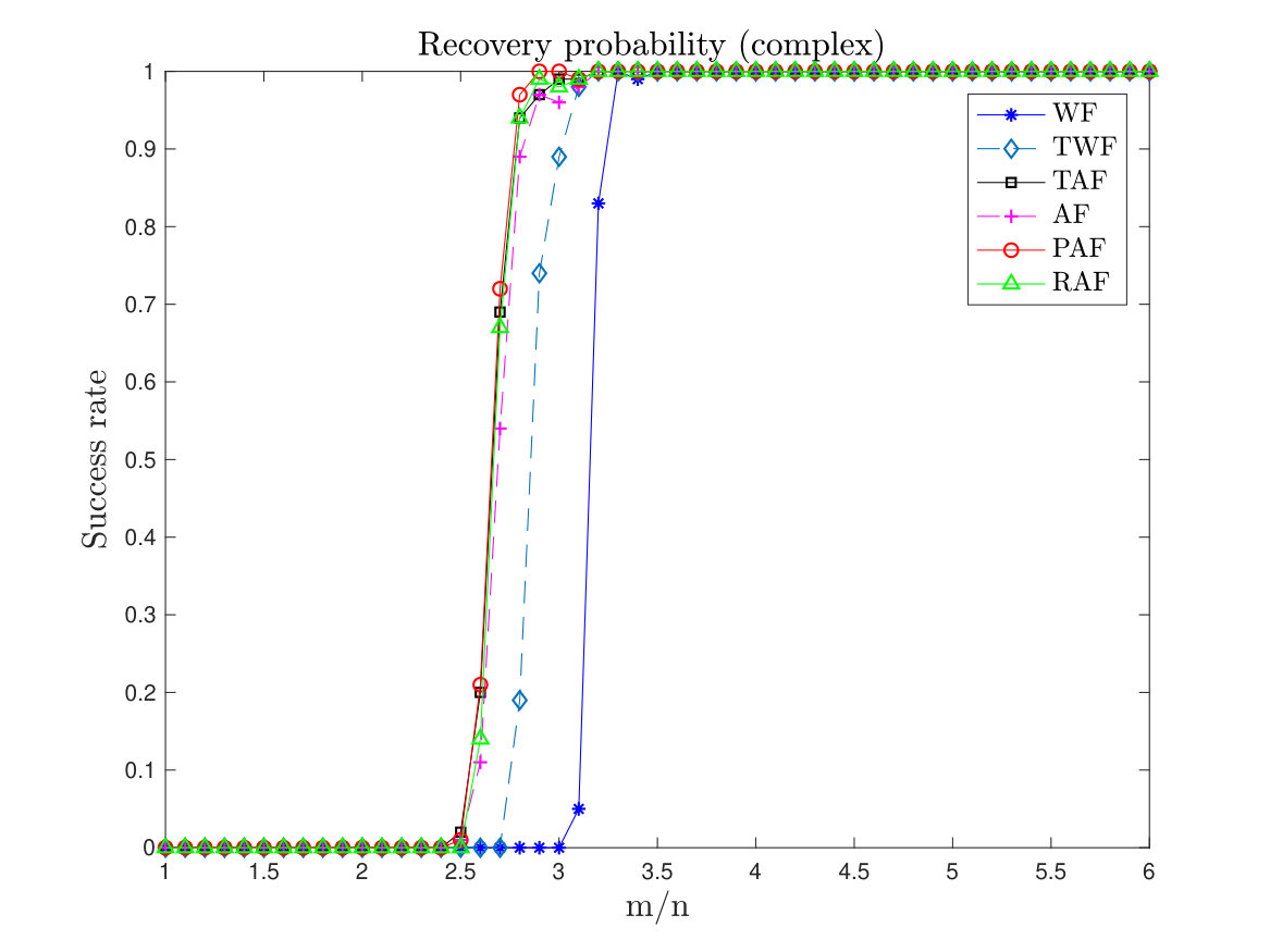 Figure 8
 Figure 9
 Figure 10
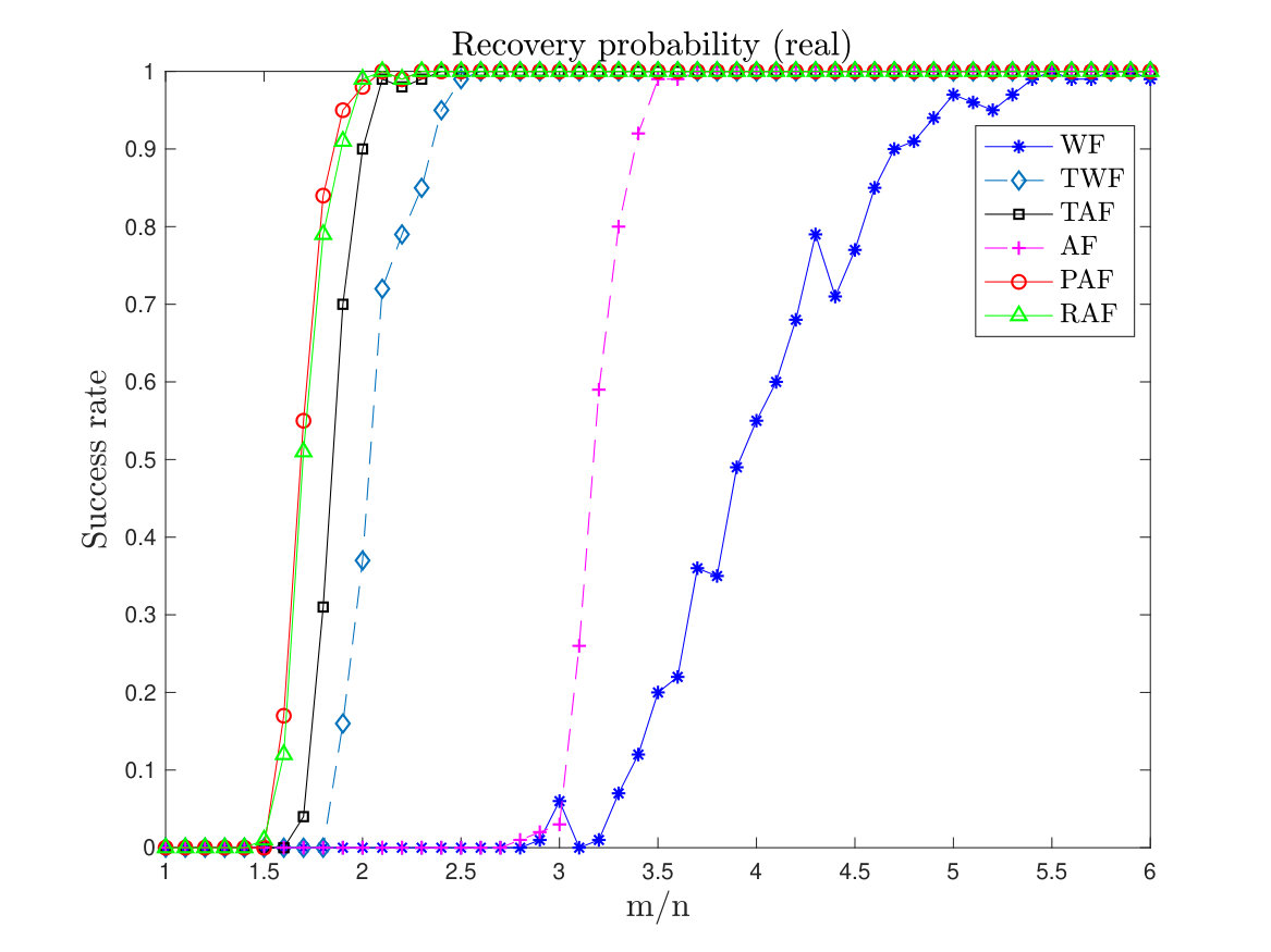 Figure 11
| Algorithm | Relative error | Iter | Time(s) |
|---|---|---|---|
| WF | 172 | 348.36 | |
| 302 | 606.71 | ||
| TWF | 51 | 320.53 | |
| 118 | 691.39 | ||
| TAF | 37 | 118.06 | |
| 84 | 250.23 | ||
| RAF | 37 | 124.99 | |
| 84 | 271.40 | ||
| PAF | 37 | 97.27 | |
| 84 | 224.23 | ||
| AF | 37 | 87.65 | |
| 84 | 189.24 |
Peer Reviews
No public reviews on file for this paper yet. If you reviewed it on a platform where reviews are public (OpenReview, ICLR, NeurIPS, ICML), you can paste yours below so the community can read it here.
Code & Models
Videos
No videos yet. Explain this paper in a talk, walkthrough, or lecture? Add one.
Perturbed amplitude flow for phase retrieval
††thanks: B. Gao is with School of Mathematical Sciences, Nankai University, Tianjin, China. Email: [email protected] ††thanks: X. Sun is with Microsoft Research Asia Email: [email protected] ††thanks: Y. Wang is with Department of Mathematics, The Hong Kong University of Science and Technology, Clear Water Bay, Kowloon, Hong Kong. Email: [email protected] ††thanks: Z. Xu is with Inst. Comp. Math., Academy of Mathematics and Systems Science, Chinese Academy of Sciences, Beijing, 100091, China; School of Mathematical Sciences, University of Chinese Academy of Sciences, Beijing 100049, China. Email: [email protected] ††thanks: Yang Wang was supported in part by the Hong Kong Research Grant Council grants 16306415 and 16308518. Zhiqiang Xu was supported by NSFC grant (91630203, 11688101), Beijing Natural Science Foundation (Z180002).
Bing Gao, Xinwei Sun, Yang Wang, Zhiqiang Xu
Abstract
In this paper, we propose a new non-convex algorithm for solving the phase retrieval problem, i.e., the reconstruction of a signal ( or ) from phaseless samples , . The proposed algorithm solves a new proposed model, perturbed amplitude-based model, for phase retrieval and is correspondingly named as Perturbed Amplitude Flow (PAF). We prove that PAF can recover () under Gaussian random measurements (optimal order of measurements). Starting with a designed initial point, our PAF algorithm iteratively converges to the true solution at a linear rate for both real and complex signals. Besides, PAF algorithm needn’t any truncation or re-weighted procedure, so it enjoys simplicity for implementation. The effectiveness and benefit of the proposed method are validated by both the simulation studies and the experiment of recovering natural images.
Index Terms:
Phase retrieval, Perturbed amplitude flow, Linear convergence.
I Introduction
I-A Problem Setup and Related Work
In this paper, we consider the well-known phase retrieval problem, which aims to recover a signal , where or , from phaseless measurements
[TABLE]
Here is the target signal or the target vector and the vectors for all are the measurement vectors. Phase retrieval has many applications in both science and engineering, such as X-ray crystallography [1, 2], astronomy [3], optics [4, 5], microscopy [6].
Due to the removal of phase information in the measurements , we can only recover up to a unimodular constant. Moreover, it is also known that general measurements are enough to recover a signal uniquely. Particularly, it was shown that and generic measurements are sufficient to recover any up to a unimodular constant for and , respectively [7, 8, 9].
The original phase retrieval problem mainly considers the recovery of a signal from its Fourier transform magnitude [10] or the magnitude of the short-time Fourier transform [11, 12, 13]. At the same time, more algorithms have been developed for general cases, in which random observations are considered, which also provide heuristic algorithms for practical applications. They can be roughly divided into two categories: the convex methods and the non-convex ones. For convex methods, the general strategy is to lift the phase retrieval problem into a problem of recovering a rank-one matrix and apply the semi-definite programming to solve it. The first such method, called PhaseLift [14, 15, 16], can achieve the exact recovery using independent Gaussian random measurements , . However, such an approach is computationally inefficient for large dimensional problems since semi-definite programming for matrices is slow for large . An alternative method called PhaseMax [17, 18, 19] aims to recover the signal by solving the model
[TABLE]
where is an approximation to the true signal . It is proved that this method can recover with high probability when where . However, numerical experiments have shown that larger oversampling ratios are often required for exact recovery, especially compared to several non-convex algorithms.
In a different direction, a series of non-convex approaches have been proposed and studied. Among such schemes, early studies are based on the alternating projection approach, including the works by Gerchberg and Saxton [20] and Fineup [21]. These methods often perform well numerically but lack theoretical foundations. Motivated by the success of alternating minimization, Netrapalli et al [22] developed the AltMinPhase method that is shown to achieve linear convergence with Gaussian random measurements and resampling. Recently, the sample complexity is improved to Gaussian random measurements in complex number field under a carefully chosen initial point by Waldspurger in [23]. However, such an alternating projection-based approach also suffers from larger computational complexity, due to the projection step. More recently another framework was proposed, in which one starts from a “good” initial guess and try to iteratively refine it by solving a given model such as the intensity-based model [24, 25]
[TABLE]
or the amplitude-based model [26, 27, 28, 29]
[TABLE]
or the Poisson likelihood model [30]
[TABLE]
Among existing proposed algorithms to solve intensity-based model (2), Candès et al have developed the Wirtinger Flow method (WF) [24] to recover via gradient descent. It achieved provable linear convergence with Gaussian random measurements under carefully chosen initialization method. Particularly, Sun et al [31] proved the benign geometric landscape of (2) under Gaussian measurements, motivating the Trust-region method to avoid spurious local minimizers. Besides, Ma et al [32] proved the “nice” geometry of (2) under Gaussian random measurements, explaining the favorable performance of unregularized gradient descent. Such geometric benefits guarantee the success of gradient descent for this non-convex phase retrieval problem. Recently, the result is refined in real field to achieve a reduction of measurements by solving amplitude-based model (3) via gradient descent [27] or via truncated gradient descent [26] or via reweighted gradient descent [29], or by solving Poisson likelihood model (4) via modified gradient descent [30]. In detail, Zhang et al [33] have proposed Reshaped Wirtinger Flow, which named Amplitude Flow (AF) in this paper to coincide with the model used, to solve model (3) by gradient descent. Wang et al [26] have proposed Truncated Amplitude Flow (TAF) to solve model (3) by truncated gradient descent. Wang et al [29] have designed Reweighted Amplitude Flow (RAF) to solve model (3) via reweighted gradient descent. Chen and Candès [30] have designed Truncated Wirtinger Flow (TWF), which solves model (4) by modified gradient descent.
From the perspective of theoretical analysis, the methods that given in AF, TAF, RAF and TWF all can achieve linear convergence under the optimal order of measurements. Different from truncation-based methods (e.g., TAF [26], TWF [30]) that remove the components having too much influence on the search direction, the RAF [29] implements re-weighted procedure to control such components by reducing their weights at each update. Instead of using truncation or re-weighted procedures to get reliable gradients, the AF [27] method performs gradient descent directly. But the analysis of AF is based on the fact that the value of equals or , which can only be satisfied in the real number field. This fact is also required by TAF, TWF and RAF. Thus the theoretical results can’t be extended to the complex case trivially.
In this paper, we introduce a new perturbed amplitude-based model to address these theoretical deficiencies and limitations in this framework.
I-B Our Contribution: The Perturbed Amplitude Flow (PAF)
We propose the Perturbed Amplitude Flow (PAF) algorithm in this paper through the following model:
[TABLE]
where have prescribed value, with the requirement that
[TABLE]
Note that if , then is smooth regardless of the value of , even when . The loss function is thus smooth. When all , this model is reduced to the classic amplitude-based model (3). So we shall name it as the perturbed amplitude-based model and name the corresponding gradient descent method as Perturbed Amplitude Flow (PAF).
In the perturbed amplitude-based model (5), not only keeps the loss function smooth but plays a role similar to truncation/re-weighted while reducing the effects of bad observations. From the previous work [26, 29], we know that only the gradients associated with sizable offer meaningful directions. In detail, considering the model (3), when the wirtinger derivative of concerning to is
[TABLE]
with . Note that the first term flows a desirable direction, whereas the second term {\mathbf{a}}_{j}|{\mathbf{a}}_{j}^{\top}{\mathbf{x}}|\Big{(}\frac{{\mathbf{a}}_{j}^{\top}{\mathbf{x}}}{|{\mathbf{a}}_{j}^{\top}{\mathbf{x}}|}-\frac{{\mathbf{a}}_{j}^{\top}{\mathbf{z}}}{|{\mathbf{a}}_{j}^{\top}{\mathbf{z}}|}\Big{)} has negative influence and such an influence can be reduced when shares the same sign with . The TAF [26] established that those terms with inconsistent sign are normally those terms with small in real case, which motivates a truncation scheme that drops the terms with small . Instead of abandoning those gradients, RAF [29] uses re-weighted procedure to reduce the influence of those components. However, these analyses heavily rely on the sign of each element equal 1 or -1, therefore hard to be extended to the complex case.
For our model, with a suitable choice of , one can control the size of the gradient. This is essential for avoiding the extremely large gradient components. More precisely, note that the Wirtinger derivative of with respect to is
[TABLE]
The magnitude of is under control even when very small. This fact avoids the extreme value of gradients during each update, which makes each update flows in a desirable direction and guarantees the gradient satisfies curvature condition. The curvature condition shall be introduced in Lemma II.3.
So the truncation-based methods (TAF, TWF) use truncation to withdraw the spurious components and RAF uses re-weighted to reduce the effects of “bad” gradients. Compared to them, our PAF controls these components by adding the perturbed term, i.e., to avoid the extreme value during each update, which frees our methods from truncation or re-weighted procedure. Besides, such a perturbation and corresponding benefit is applicable to both real and complex fields, thus make our theoretical analysis easily incorporate the complex field as a whole.
Numerical tests show that our proposed algorithm outperforms AF () in terms of success rate for real signals, as shown in Figure 2. Besides, using vanilla gradient descent to solve the perturbed amplitude-based model (5), we can achieve linear convergence with measurements for both real and complex signals (see Section II). The result improves upon the WF method, which uses measurements, or the AF method, which can be theoretically proved only for real signals, or the TWF, TAF, RAF methods, which need truncation or re-weighted procedure during each iteration.
In summary, compared with the previous algorithms for solving model (3) or (4), the PAF method needn’t truncation or re-weighted at all and the convergence result holds for both real and complex signals. Numerical experiments show that the proposed PAF method is slightly more efficient although comparable computationally with TAF, RAF and significantly more efficient than TWF (see Section III). We believe the reason lies in the fact that truncated/re-weighted methods, such as TWF, TAF, RAF incur additional computational cost on measuring the gradient components.
I-C Notations
Let or be the target signal. Throughout this paper, we assume that , are independent and identically distributed standard Gaussian random measurement vectors, i.e. for and for . For each measurement , we obtain . We shall attempt to recover the original signal from , by solving the perturbed amplitude-based model (5). In this paper, we use , or the subscript/superscript form of them to represent constants and their values vary according to the context. Since for phase retrieval the best we can do is to recover the target signal up to a global phase/sign, we use the following definition for distance between two vectors :
[TABLE]
where
[TABLE]
For any , we define the -neighborhood of as
[TABLE]
II Perturbed Amplitude Flow Algorithm
II-A Initialization
To avoid iterations getting trapped in undesirable stationary points, a proper initialization is essential to any non-convex optimization problem. To achieve this goal, many initialization methods have been proposed, such as the spectral initialization method [24], a modified spectral initialization method [30] and the null initialization method [26]. These methods are all based on finding the eigenvector corresponding to the largest eigenvalue of a specially designed Hermitian matrix.
Here we adopt the initialization strategy given in [25], which is shown to provide a good initial guess under measurements. With this strategy, the initial guess is obtained by calculating the eigenvector corresponding to the largest eigenvalue of the Hermitian matrix
[TABLE]
with for or for , and normalized to , where is defined by
[TABLE]
Lemma II.1** ([25]).**
Let be the above initial guess. For any , there exists a such that for ,
[TABLE]
holds with probability at least .
II-B Gradient Descent Iteration
After initialization to obtain , we use gradient descent on the loss function given in (5) by
[TABLE]
to iteratively refine the estimation:
[TABLE]
where is the step size and is the Wirtinger derivative of with respect to in complex variables which is defined as
[TABLE]
As simple as the scheme (10) may look, our main result proves that it can achieve linear convergence under the optimal order of measurements by choosing for an appropriately chosen parameter ().
Motivated by the technique used in WF, the proof of our main result is mainly based on the following two key lemmas, whose proofs are given in Section IV.
Lemma II.2**.**
Let be the target signal and assume that satisfies (6). For any , there exist constants , such that as long as , then with probability at least ,
[TABLE]
holds for every satisfying .
This lemma implies that the gradient of is well controlled in the neighborhood of the target signal .
Lemma II.3**.**
Let be the target signal and assume that with . There exist positive constants depending on such that for any and , we have
[TABLE]
with probability at least .
The constants in the lemma can, in theory, be explicitly estimated, although the theoretical estimates are typically “overkills” for practical applications, just like in other existing schemes. Later in Remark IV.1, we show more explicitly the relation between and . Particularly, by setting , roughly reaches its largest value. For with , Lemma II.3 guarantees sufficient descent along the search direction.
Set with . Then
[TABLE]
The main technique in proving Lemma II.3 is that we first fix one and then provide estimates separately for cases and . An -net argument is then used to obtain uniform control over all .
Building on these two lemmas, we can now state and prove our main theorem, which establishes linear convergence of the PAF algorithm iteration (10).
Theorem II.1**.**
Under the conditions of Lemma II.3, let , be the iterations generated by (10) with . Assume that . Then there exist positive constants such that for , with probability at least , the following holds for all
[TABLE]
In particular by taking , with probability at least , the following holds for all
[TABLE]
Proof:
According to the update rule (10), Lemma II.2 and Lemma II.3, for , with probability at least we have
[TABLE]
This establishes the linear convergence part of the theorem.
For the second part, we set . Later in Remark IV.1, we show that one may take in . Substituting these values in we thus obtain
[TABLE]
∎
As mentioned earlier, we can achieve through initialization given in Lemma II.1, by setting . This also requires measurements. Thus the combination of Lemma II.1 and Theorem II.1 yield linear convergence of the PAF algorithm.
III Numerical Experiments
III-A Simulation Study
To evaluate the performance of our PAF algorithm, we present a series of simulated tests and compare them with WF, TWF, AF, TAF and RAF. We perform all the simulations under the same initialization procedure. All experiments are carried out on Matlab 2017b with a 2.3 GHz Intel Core i5-8259U and 16 GB memory.
First we plot the relative error for the recovery of a complex-valued signal, in logarithmic scale versus the iteration count for WF, TWF, AF, TAF, RAF and PAF. We choose with i.i.d. Gaussian random measurements . For the initialization, we follow the method given in Section II-A with 50 power iterations. For the PAF algorithm we set and fix the step size . Note that AF is equivalent to PAF algorithm with . We also consider the case where the measurements are contaminated by noise, i.e. where the noise follows distribution . The results are plotted in Figure 1. It shows that PAF, TWF, AF, TAF and RAF, all of which converge linearly in theory, have comparable convergence rate. PAF seems to have a slight advantage possibly due to its ability to handle a larger step size.
Next, we compare the empirical success rate of PAF with that of WF, TWF, AF, TAF and RAF. Here we set the maximum number of gradient-type iterations to for each scheme. In PAF, we set , and fix the step size to . We let vary from to . A test is successful if the relative error is within after the maximum number of iterations. For the test we compute the success rate by performing 100 random trials for each . The results are given in Figure 2. Of particular note is that in the real case, PAF, TWF and TAF all perform better than AF, indicating the effectiveness of controlling the size of the gradient in all gradient descent algorithms for avoiding spurious stationary points. WF seems to lag behind other algorithms, unsurprisingly, as it agrees with the theoretical analysis.
III-B Recovery of Natural Image
To show the efficiency and scalability of our algorithm, we use PAF to recover the Milky Way Galaxy image 111Download from http://pics-about-space.com/milky-way-galaxy, which is the image used in [24, 34] with the coded diffraction measurements. We denote the image by , . This is a color image so it has three channels. Thus we actually perform phase retrieval for each of the three channels separately. Let denote any of the color channels of . We have measurements
[TABLE]
where denotes the discrete Fourier transform matrix, and is a diagonal matrix having i.i.d. entries sampled from a distribution . Here we take the *octanary * pattern that , where and are independent with distributions
[TABLE]
and
[TABLE]
We set and adopt the same initialization method for all schemes in our comparison. For each model, we record the time elapsed and the iterations needed to achieve relative error at and , respectively. The results are shown in Table I. It is shown that PAF achieves the same level of precision and is comparable in efficiency with AF and TAF. Besides, note that it took TAF, RAF, PAF and AF the same number of iterations to achieve fixed relative error. Moreover, it’s reasonable that our PAF is a little bit slower than AF () with additional nonzero item . These three methods are significantly more efficient than WF and TWF.
Interestingly if we take a much smaller , while WF does not recover the target image, our PAF method actually performs better than with . It takes 300 iterations and computation time sec to achieve recovery with a relative error of in Figure 3. While more iterations are taken here, the computational time is actually less because is significantly smaller than .
IV Proof of main lemmas in section II-B
IV-A Proof of Lemma II.2
Proof:
For any , set , where we recall that is given in (8). Then . Denote , with . Note that we set if . Then . For any , we have
[TABLE]
where the last inequality follows from the inequality for any . According to Lemma .1 (see the Appendix), for any and with a sufficiently large constant , the inequality
[TABLE]
holds with probability at least for some . Also for the Gaussian random matrix and any , for we have with probability at least ([35], Remark 5.40). These results together imply that
[TABLE]
holds with probability at least whenever for some . Here we choose and . ∎
IV-B Proof of Lemma II.3
Proof:
Without loss of generality, we shall assume that the target signal has . Again for each we set , and denote . Definition 7 implies that . Since , we have . Therefore
[TABLE]
with being the -th item of the summation. To simplify the statement, we use to denote the denominator of , i.e.,
[TABLE]
To prove the conclusion holds for all , i.e., any in unit ball. We first consider to be fixed and then divide it into two cases.
In the first case, we assume with . Here we have , which implies . Hence
[TABLE]
due to the facts that
[TABLE]
and . Thus under the condition of , we obtain
[TABLE]
By Lemma .1 of the Appendix, for , with probability greater than we have
[TABLE]
For the second case , given the assumption and , we claim that
[TABLE]
Indeed, for each measurement we have
[TABLE]
Also note that a Gaussian random measurement is rotational invariant, i.e. for any unitary matrix , is also a Gaussian random measurement. Thus for fixed and , we may without loss of generality assume that and , with . This is because otherwise we can always find a unitary matrix to map to these two vectors. Set
[TABLE]
where is unitary and
[TABLE]
Then we have and . Set and is a Gaussian random measurement. Consequently we have
[TABLE]
which implies
[TABLE]
Combining (15) and (16) we now obtain (14).
For each index set , define a corresponding event
[TABLE]
According to (14), we know that the event occurs with probability . We assume that is an index set which satisfies . Then on event , {\rm Re}\big{(}\langle\nabla f_{{\bm{\epsilon}}}({\mathbf{z}}),\,{\mathbf{z}}-{\mathbf{x}}e^{i\phi_{\mathbf{x}}({\mathbf{z}})}\rangle\big{)} can be divided into two groups:
[TABLE]
For each group, we next provide an upper bound and a lower bound for the denominators , . Recall that . When j\in I_{0}=\big{\{}j\,:\,\rho\,|{\mathbf{a}}_{j}^{*}{\mathbf{x}}|>|{\mathbf{a}}_{j}^{*}{\mathbf{h}}|\big{\}} we have
[TABLE]
where . Here the second inequality follows from and
[TABLE]
On the other hand, since
[TABLE]
and , we have
[TABLE]
where L_{1}:=\sqrt{(1-\rho)^{2}+\alpha}\,\big{(}\sqrt{(1-\rho)^{2}+\alpha}+\sqrt{1+\alpha}\big{)}/\rho^{2}. Similarly, for k\in I_{0}^{c}=\big{\{}k\,:\,\rho\,|{\mathbf{a}}_{k}^{*}{\mathbf{x}}|\leq|{\mathbf{a}}_{k}^{*}{\mathbf{h}}|\big{\}}, we have
[TABLE]
and hence
[TABLE]
where and
[TABLE]
where .
Using the concentration inequalities given in the Appendix, we next give the lower bounds of and . Based on (17), (18) and Lemma .3, given any , for the following inequality holds with probability at least 1-\exp\big{(}-c_{1}(\delta)\cdot|I_{0}|\big{)}
[TABLE]
where . Here the fourth inequality comes from Lemma .3.
Similarly, according to (19), (20) and Lemma .3, for the following inequality holds with probability at least 1-\exp\big{(}-c_{2}(\delta)\cdot|I_{0}^{c}|\big{)}:
[TABLE]
where \phi=\Big{(}\frac{3}{4U_{2}\rho}\Big{)}^{2}/\Big{(}\frac{63}{128U_{2}\rho^{2}}-\frac{9}{128L_{2}}\Big{)} and . The second inequality follows from the concentration inequalities given in Lemma .3. The fourth inequality derives from the facts that for any and .
Set . For arbitrary fixed , a simple observation is that and are decreasing functions of . So we next only consider . When , we have
[TABLE]
and
[TABLE]
with .
For sufficiently large constant , as long as , we have and . Thus with probability at least , we have
[TABLE]
The number of the index sets satisfying is . So for fixed , when , the inequality (LABEL:generalcase) holds with probability greater than . Note that
[TABLE]
and . Hence for some , which implies that . Moreover, for we have
[TABLE]
Considering the two cases as a whole, for a fixed , combining (LABEL:specialcase), (LABEL:generalcase) and (24), we obtain
[TABLE]
with probability at least . Particularly, when we have .
To complete the proof, we will need to establish uniform bound over all vectors, so we adopt an -net argument. Observe that
[TABLE]
For any , which means for any with and , we consider the function {\rm Re}\big{(}\langle\nabla f_{\bm{\epsilon}}({\mathbf{x}}+\rho\tilde{{\mathbf{h}}}),\,\rho\tilde{{\mathbf{h}}}\rangle\big{)} with . Suppose that satisfy . When we have
[TABLE]
where . Here the third inequality follows from Lemma II.2 and Lemma .4. Therefore for any and satisfying with , let be an -net for the unit sphere of with cardinality . Then for all , and , with probability at least we have
[TABLE]
with . According to Remark IV.1, when , approximately reaches its largest value. ∎
Remark IV.1**.**
According to the proof of Lemma II.3, by taking and , we have , , and . Recall that
[TABLE]
with . Figure 4 here shows the relationship between and .
Particularly, when , roughly reaches its maximum.
[Auxiliary Lemmas]
In previous sections we have applied concentration inequalities several times. They have played a key role in the proof of our results. Here we present these concentration inequalities used for the proof of Lemma II.2 and Lemma II.3.
Lemma .1** ([14] Lemma 3.1 ).**
Let be i.i.d. Gaussian random measurements. Fix any in and assume . Then for all unit vectors ,
[TABLE]
holds with probability at least , where .
Lemma .2**.**
Let be a Gaussian random measurement. Let and be two fixed vectors with , and . Then we have
[TABLE]
[TABLE]
[TABLE]
[TABLE]
and
[TABLE]
Proof:
Since the distribution of is invariant by unitary transformation, we can take and , where and . We use to represent the real and imaginary parts of and respectively, which implies that the variables are independent and obey normal distribution . Then it follows that
[TABLE]
[TABLE]
and
[TABLE]
Since is invariant by unitary transformation and are two fixed vectors satisfying , so we have
[TABLE]
Here is a Gaussian random measurement with unitray matrix satisfying and . Then we obtain
[TABLE]
which implies (LABEL:exp-haax).
Similarly, we have
[TABLE]
which implies
[TABLE]
[TABLE]
And
[TABLE]
implies
[TABLE]
and
[TABLE]
Then to prove the inequalities (27), (28), (29) and (30), it’s sufficient to prove
[TABLE]
[TABLE]
Next, we commit to prove (31) and (32). Firstly, we take polar coordinates transformation:
[TABLE]
with , . Then we can write the expectation as
[TABLE]
It is an even function about and when the derivative
[TABLE]
Hence the expectation obtains its maximum at , i.e.,
[TABLE]
Thus we have the inequality (31).
Using the same polar coordinates transformation, we know
[TABLE]
Thus we obtain (32). This completes the proof. ∎
Lemma .3**.**
Let be i.i.d. Gaussian random measurements. Let and be two fixed vectors with , and . For any , there exist positive constants such that for any the inequalities
[TABLE]
[TABLE]
[TABLE]
[TABLE]
and
[TABLE]
hold with probability at least .
Proof:
For fixed and , the following sets are all independent sub-exponential random variables
[TABLE]
[TABLE]
[TABLE]
[TABLE]
[TABLE]
Recall that is a Gaussian random measurement. Then based on Bernstein-type inequality, for any , the inequalities
[TABLE]
[TABLE]
[TABLE]
[TABLE]
[TABLE]
hold with probability at least provided , where are positive constants depending on . Then the inequalities (33), (34), (35), (LABEL:con3), (LABEL:con4) can be derived directly from the expectation bounds given in Lemma .2.
∎
The following lemma provides an upper bound for the operator norm of .
Lemma .4**.**
Set . Then there exist constants such that for , holds with probability at least .
Proof:
Recall that
[TABLE]
Similarly, we obtain
[TABLE]
For any , we have
[TABLE]
with probability at least provided . Here the third inequality is obtained by Lemma .1. ∎
The reference list from the paper itself. Each links out to its DOI / PubMed record.
- 1[1] J. Miao, P. Charalambous, J. Kirz, and D. Sayre, “Extending the methodology of x-ray crystallography to allow imaging of micrometre-sized non-crystalline specimens,” Nature , vol. 400, no. 6742, p. 342, 1999.
- 2[2] V. Elser, T. Lan, and T. Bendory, “Benchmark problems for phase retrieval,” Siam Journal on Imaging Sciences , vol. 11, no. 4, pp. 2429–2455, 2018.
- 3[3] C. Fienup and J. Dainty, “Phase retrieval and image reconstruction for astronomy,” Image Recovery: Theory and Application , pp. 231–275, 1987.
- 4[4] A. Walther, “The question of phase retrieval in optics,” Optica Acta: International Journal of Optics , vol. 10, no. 1, pp. 41–49, 1963.
- 5[5] R. P. Millane, “Phase retrieval in crystallography and optics,” JOSA A , vol. 7, no. 3, pp. 394–411, 1990.
- 6[6] J. Miao, T. Ishikawa, Q. Shen, and T. Earnest, “Extending x-ray crystallography to allow the imaging of noncrystalline materials, cells, and single protein complexes,” Annu. Rev. Phys. Chem. , vol. 59, pp. 387–410, 2008.
- 7[7] R. Balan, P. Casazza, and D. Edidin, “On signal reconstruction without phase,” Applied and Computational Harmonic Analysis , vol. 20, no. 3, pp. 345–356, 2006.
- 8[8] A. S. Bandeira, J. Cahill, D. G. Mixon, and A. A. Nelson, “Saving phase: Injectivity and stability for phase retrieval,” Applied and Computational Harmonic Analysis , vol. 37, no. 1, pp. 106–125, 2014.
