TL;DR
This paper introduces a novel deep learning method using Spatial-GANs to generate large, realistic synthetic astronomical images that closely resemble real deep field observations, enabling scalable data simulation.
Contribution
The authors demonstrate the application of Spatial-GANs to produce arbitrarily large, high-fidelity synthetic astronomical images, advancing data-driven simulation techniques in astrophysics.
Findings
Generated images match real data in galaxy properties
Created a 7.6-billion pixel synthetic deep field
Method generalizes to other imaging datasets
Abstract
Generative Adversarial Networks (GANs) are a class of artificial neural network that can produce realistic, but artificial, images that resemble those in a training set. In typical GAN architectures these images are small, but a variant known as Spatial-GANs (SGANs) can generate arbitrarily large images, provided training images exhibit some level of periodicity. Deep extragalactic imaging surveys meet this criteria due to the cosmological tenet of isotropy. Here we train an SGAN to generate images resembling the iconic Hubble Space Telescope eXtreme Deep Field (XDF). We show that the properties of 'galaxies' in generated images have a high level of fidelity with galaxies in the real XDF in terms of abundance, morphology, magnitude distributions and colours. As a demonstration we have generated a 7.6-billion pixel 'generative deep field' spanning 1.45 degrees. The technique can be…
Click any figure to enlarge with its caption.
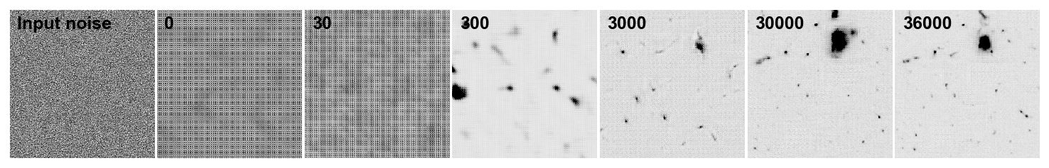 Figure 1
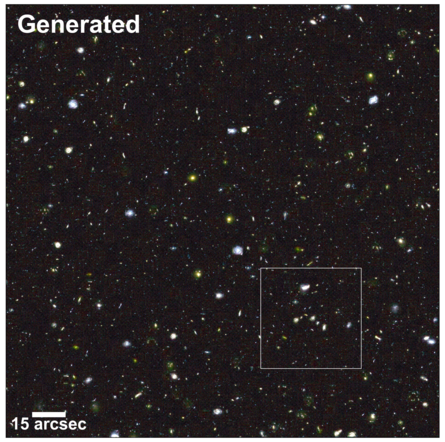 Figure 2
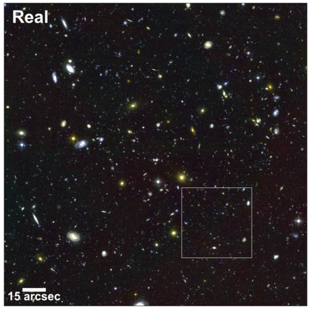 Figure 3
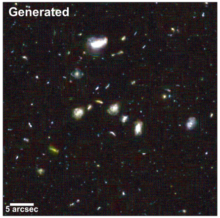 Figure 4
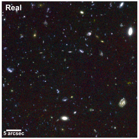 Figure 5
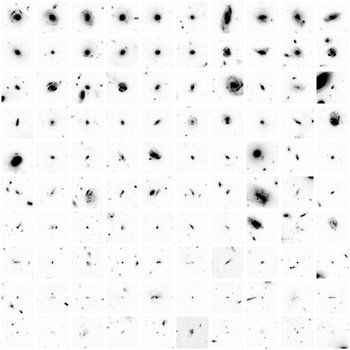 Figure 6
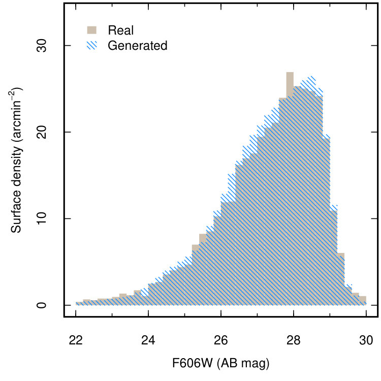 Figure 7
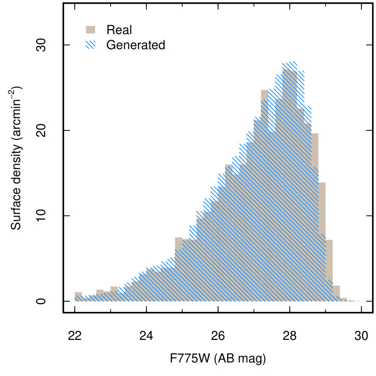 Figure 8
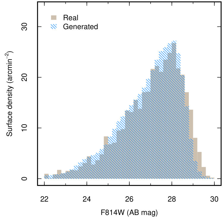 Figure 9
Peer Reviews
No public reviews on file for this paper yet. If you reviewed it on a platform where reviews are public (OpenReview, ICLR, NeurIPS, ICML), you can paste yours below so the community can read it here.
Code & Models
Videos
No videos yet. Explain this paper in a talk, walkthrough, or lecture? Add one.
Generative deep fields: arbitrarily sized, random synthetic astronomical images through deep learning
Michael J. Smith & James E. Geach
Centre for Astrophysics Research, School of Physics, Astronomy & Mathematics, University of Hertfordshire, Hatfield, AL10 9AB
Centre of Data Innovation Research, School of Physics, Astronomy & Mathematics, University of Hertfordshire, Hatfield, AL10 9AB [email protected]@herts.ac.uk
Abstract
Generative Adversarial Networks (GANs) are a class of artificial neural network that can produce realistic, but artificial, images that resemble those in a training set. In typical GAN architectures these images are small, but a variant known as Spatial–GANs (SGANs) can generate arbitrarily large images, provided training images exhibit some level of periodicity. Deep extragalactic imaging surveys meet this criteria due to the cosmological tenet of isotropy. Here we train an SGAN to generate images resembling the iconic Hubble Space Telescope eXtreme Deep Field (XDF). We show that the properties of ‘galaxies’ in generated images have a high level of fidelity with galaxies in the real XDF in terms of abundance, morphology, magnitude distributions and colours. As a demonstration we have generated a 7.6-billion pixel ‘generative deep field’ spanning 1.45 degrees. The technique can be generalised to any appropriate imaging training set, offering a new purely data-driven approach for producing realistic mock surveys and synthetic data at scale, in astrophysics and beyond.
keywords:
methods: miscellaneous, methods: statistical, surveys
††pubyear: 2019††pagerange: Generative deep fields: arbitrarily sized, random synthetic astronomical images through deep learning–LABEL:lastpage
1 Introduction
Synthetic, or mock, data plays an important role in the interpretation of observations, as it provides a means to test a theoretical framework, as a tool to explore biases or systematics in data analysis, or to help design future experiments. In astrophysics, like many fields, a standard route to generating synthetic data is to use an analytic or semi-analytic model, or numerical simulation, to generate synthetic data that mimic the observations (e.g., Cole et al., 1998; Obreschkow et al., 2009; Mandelbaum et al., 2012). The most common form of observation in astrophysics is digital imaging, and deep extragalactic imaging surveys have transformed our understanding of the Universe (Williams et al., 1996; Scoville et al., 2007).
Current methods to generate synthetic deep fields include the projection of volume- and resolution-limited hydrodynamical cosmological simulations (e.g., Schaye et al., 2015; Vogelsberger et al., 2014) into lightcones (Snyder et al., 2017), requiring a treatment for the transport of radiation through the volume and modelling of a particular instrument response (Jonsson, 2006; Trayford et al., 2017). Alternatively, mock deep fields can be created by taking an input catalogue containing the positions and properties of fake galaxies and applying models to describe their light profiles (Bertin, 2009; Dobke et al., 2010; Rowe et al., 2015). However, with a large, representative data set, an alternative approach is to use empirical data itself to construct new, realistic, but synthetic observations.
Generative Adversarial Networks (GANs) are a type of deep learning algorithm that can generate new samples from a probability distribution learnt from a representative training set (Goodfellow et al., 2014). The adversarial aspect of the algorithm refers to the use of two neural networks – a generator, and discriminator, – that compete during training. tries to estimate the probability distribution of the input data by producing samples that aim to trick , which is estimating the probability that the generated sample came from the training set. Training is a ‘minimax’ game where is trying to maximize the likelihood that predicts the generated samples are from the real data. The generator transforms a ‘latent’ vector , into an output . Meanwhile, the discriminator takes either the output of the generator , or a real data example , and transforms this input into an output, or . The output can be thought of as the probability that is indistinguishable from . The networks are trained through gradient descent (Robbins & Monro, 1951) until ’s distribution closely matches the distribution of . After training, the generator can produce convincing images resembling those in the training set. These generated images can be thought of as random draws from the probability distribution estimated by the generator that describes the distribution from which pixels in the training image were sampled.
In this work we present a method exploiting GANs to generate realistic, but random, extragalactic deep field images of arbitrary size. In Section 2 we describe the ‘Spatial GAN’ variant, and explain how it is trained to generate fake images. In Section 3 we describe our results, comparing ‘galaxies’ detected in the fake images to galaxies detected in the training image. We discuss and summarise the results and highlight limitations and scope for improvement and future work in Section 4. Magnitudes are all quoted on the AB system.
2 Method
2.1 Spatial–GANs
A Spatial–GAN (SGAN, Jetchev et al., 2016) is a fully convolutional GAN that uses variably sized 2D latent vector arrays as the generator input . This is in contrast to a standard GAN, which uses a 1D latent vector. In a standard GAN a dense neural layer is used to connect and reshape the latent vector so that a convolutional layer can operate on it. This lack of a fully-convolutional architecture means that a standard GAN can only produce images of a single, fixed shape. An SGAN replaces all dense neural layers in both its generator and its discriminator with convolutional layers. This allows input of variably sized image–latent vector array pairs. In an SGAN the latent vector arrays are upsampled using deconvolving layers in the generator, and both generated and real images are downsampled in the discriminator via convolving layers. Since can be varied, an SGAN can be used to create an image of any size, even one much larger than seen in the training set. If the training images exhibit periodicity, the SGAN’s generator will also learn to exhibit the same periodicity (Jetchev et al., 2016).
2.2 Training set
We use a training set comprised of the F814W, F775W and F660W bands of the Hubble Space Telescope eXtreme Deep Field (XDF, Illingworth et al., 2013), with all images aligned and sampled on the same 60-mas grid111https://archive.stsci.edu/prepds/xdf. The only other preprocessing is a channel-wise clip at the 99.99th percentile. Unlike many GAN approaches that use training images scaled to an 8-bit depth per channel, we train using the full floating point dynamic range of the data, with 32-bit depth per channel. Training images are sampled from the full XDF image by cropping the image at random positions with crop sizes of 64, 128 or 256 pixels, with the size fixed for each batch. Corresponding noise arrays of sizes 4, 8, or 16 pixels, are sampled from a Gaussian distribution with a zero mean and unity variance, and passed to the generator. Each noise array has a channel axis of size 50.
2.3 Architecture and training
The generator is comprised of one initial deconvolutional layer with a stride of 2 and a kernel size of 4. Three deconvolutional sets are then applied, each comprising of one layer with a stride of 2, followed by three layers with strides of 1. Each layer in these sets have kernel sizes of 4. These layers have an exponential linear unit (ELU) activation (Clevert et al., 2016). The generator’s output layer is also deconvolutional, with a stride of 1, a kernel size of 3, and 3 filters. The output layer has a sigmoid activation function,
[TABLE]
The discriminator comprises of 5 initial convolutional layers, each with a stride of 2, and a kernel size of 4. All initial layers have a Leaky Rectified Linear Unit (ReLU) activation (Maas et al., 2013). 2D global average pooling is applied to the final convolutional layer, and a dense layer is used to connect the global average pool to a binary classification output.
The discriminator uses a relativistic average loss (Jolicoeur-Martineau, 2018). A relativistic discriminator estimates whether the incoming data are more realistic than a random sample of the opposing type. To understand why this is important, consider that in a standard GAN a perfect generator will cause the discriminator to define all incoming data as ‘real’. However, it is known that exactly half of an incoming batch is real data. Therefore, if the generator is producing flawless fakes, the discriminator should assume that each sample has a 50% probability of being real (Jolicoeur-Martineau, 2018). To take this prior knowledge into account, the output function of a non-relativistic discriminator is modified from , where is the output of the final layer with no applied activation function, to
[TABLE]
where is the sigmoid activation function. The second parts of the real and generated are effectively the average discriminator value for fake images, , and real images, , respectively. The use of a relativistic discriminator leads to stable training on a difficult data set of large images, where a standard discriminator fails (Jolicoeur-Martineau, 2018). The discriminator is packed to stabilize training (Lin et al., 2018). To pack the discriminator, two images from the same class are concatenated along their channel axes and fed into the discriminator as a single sample. Packing the discriminator in this way reduces the possibility of mode collapse (Lin et al., 2018). The Adam optimizer (Kingma & Ba, 2015) is used, with a learning rate of 0.0002. The learning rate was determined through a manual search as the maximum rate that yields stable training.
The SGAN is trained on an NVIDIA Tesla K40c GPU for 36,000 epochs of 30 batches with a batch size of 128. Each epoch requires approximately 120 seconds, depending on the batch crop sizes. The evolution of the generated images for a fixed latent noise vector is shown in Figure 1, showing the emergence of amorphous structure and then refinement into structures resembling galaxies with increasing training time.
3 Results
A self-ensemble of 21 GANs is created by taking every tenth epoch’s model from a range of 200 epochs. A Convolutional Neural Network (CNN) ensemble is a combination of different CNNs trained from different weight initialisations on the same data. A self-ensemble is an ensemble of CNNs trained from the same initialisation, but taken at different points in the training cycle. Ensembles of CNNs can produce significantly more accurate predictions when compared to a single CNN (Nanni et al., 2018; Paul et al., 2018). This increase in accuracy has been shown by Wang et al. (2016) and Mordido et al. (2018) to also be present in GAN ensembles.
Four outputs were taken from each of these 21 GANs, resulting in 84 total XDF simulations. To generate a simulation set, each of the trained generators is fed a vector that has shape , where is the batch size. The generators up-sample to a shape , matching the shape of the training image. The generation time for single realization of the XDF is 15 seconds for all three bands on an Intel Xeon CPU E5-2650 v3. In principle, the generated image can be of arbitrary contiguous size by using seamless tessellation. Seamless tessellation can be achieved with SGAN by having adjacent tiles and share a portion of boundary values. This creates a shared area where and have an equal output. A seamless tile is made by cropping at the midpoint of the shared noise and concatenating and . To illustrate, we have generated a contiguous 8704087040 pixel () version of the XDF that can be examined online at http://star.herts.ac.uk/jgeach/gdf.html.
Figure 2 presents an example of a generated field in comparison to the real XDF, combining the F814W, F775W and F606W bands into an RGB colour composite. We show the full field, spanning approximately 3*′, and a zoom-in of a 45′′* region for closer inspection. The generated image is reasonably convincing as an extragalactic deep field from the point of view of cursory visual inspection, although like many GAN-generated images, on closer inspection there are artifacts (such as low surface brightness features, pixelization, and discontinuities not seen in the real image) that betray the counterfeit. The GAN also cannot reproduce some of the larger galaxies with the same level of detail as the real image. Nevertheless, the generated image does contains a mixture of ‘early’ and ‘late’ type galaxies amongst a more numerous field of background sources. The early and late types have the correct color and morphology, i.e. classic red/elliptical and blue/spiral respectively, and background sources have the clumpy and disturbed morphology typically seen in the high redshift galaxy population. Figure 3 presents single-band (F775W) thumbnail images of a sample of 100 randomly chosen sources with F775W AB magnitudes in the range 21–26 mag. 50 sources are selected from the real image and 50 are selected from the generated images, but the thumbnails have been randomly shuffled in the Figure to demonstrate to the reader the visual similarity of individual galaxies in the generated and real data.
To test whether the similarity between the generated and real image is more than superficial, we extract ‘galaxies’ from the generated images and compare to those in the real XDF. We use the source finder SExtractor (Bertin & Arnouts, 1996) to detect galaxies in the combined F606W+F775W+F814W (pixelwise-mean) images, measuring the corresponding source flux in the individual bands. Sources are identified with the criteria that 5 contiguous pixels have a signal 5 above the local background. The same detection procedure is applied to the real and generated images, and the photometric zeropoints for the generated images are identical to the real data. Figure 4 compares the magnitude distribution of sources detected in the real field and ensemble of generated fields measured in each of the F606W, F775W and F814W bands. The generated and real distributions bear close statistical resemblance. The absolute difference in the generated and real median magnitudes in each of the F606W, F775W and F814W bands is within 0.02 magnitudes, and a the generated images produce the correct abundance of galaxies across the full magnitude range in every band. The p-values given by a two-sided Kolmogorov-Smirnov test for a magnitude limit of 28 mag (approximately the completeness limit of the catalogue for our detection criteria) are 0.16, 0.63 and 0.75, indicating that we cannot say with confidence that the distributions are drawn from different parent populations, and are therefore statistically similar.
4 Discussion and Conclusions
While the SGAN can produce arbitrarily-sized simulations of the XDF, there are clear limitations of this technique. The primary limitation is that the generated images are of course totally biased to the training set. The consequence is that a generated image much larger than the training data will not be cosmologically representative. This is simply because the XDF probes a volume too small to contain rare objects such as, for example, clusters of galaxies and the generator cannot produce examples of objects it has not seen. This problem is simple to alleviate by using a much larger and representative training set. In the real Universe, the positions of galaxies are correlated, even on large angular scales, due to the presence of cosmological large-scale structure.
Another limitation is that this clustering information is not present in the generated images, although correlations on the scales of the crop size will be somewhat preserved. Finally, we were not able to achieve stable training with more than three photometric bands. This issue could be resolved with more regularization: adding dropout (Srivastava et al., 2014), or spectral normalisation (Miyato et al., 2018) could allow one to generate additional bands, although at the cost of a longer training time, and a larger memory footprint during training.
An advantage of this technique is that it is empirically driven, since the data itself is used as the model. By training directly on imaging data the SGAN simultaneously encodes information about the instrumental response as well as the ‘galaxy’ population, thus circumventing the need to make modelling assumptions about either, as is the case in other approaches. The corollary to this is that in the current approach we cannot disentangle the instrument response from the underlying galaxy population, although one could envision approaches to tackle this challenge. For example, a method similar to that used by Schawinski et al. (2017), where a GAN is used to remove noise in astronomical imagery, could be employed. Specifically, a GAN with a UNet-like (Ronneberger et al., 2015) generator would learn a transformation between an image with an entangled instrument response, and one without.
Recent advances in GAN training techniques have resulted in impressively high fidelity image output (Karras et al., 2017; Brock et al., 2018; Zhang et al., 2018). Similar methods could be implemented to improve the quality of the generated deep fields. Training on a larger set of imaging data, with a increased batch size (Brock et al., 2018), may also produce more representative simulations on a deeper network. The addition of a GAN architecture that allows for control over the output, such as InfoGAN (Chen et al., 2016) or Conditional GAN (Mirza & Osindero, 2014) could also be useful when creating mock surveys because they would allow control over the frequency of particular objects of interest, or over the makeup of background noise.
This method could be used to generate at scale entirely artificial, but realistic, image realizations for the design, development, and exploitation of new surveys. For example, one could assemble large training sets for instance segmentation and classification of galaxies. In the early stages of a new survey, relatively small amounts of data could be collected, but then expanded to a level useful for training deep learning models using the generative method described here. Segmentation and classification algorithms could then be trained on the generated data, and then applied to new data, allowing far faster deployment of astronomical deep learning algorithms than would otherwise be possible, potentially accelerating the exploitation of new survey data.
Acknowledgements
M.J.S. acknowledges the hospitality of Queen’s University during much of this work. J.E.G. is supported by the Royal Society. We gratefully acknowledge the support of NVIDIA Corporation with the donation of the Tesla K40 GPU used for this research, which also made use of the University of Hertfordshire high-performance computing facility (http://uhhpc.herts.ac.uk). The SGAN code can be obtained at https://github.com/Smith42/XDF-GAN. The 7.6-billion pixel version of the generated XDF can be viewed at http://star.herts.ac.uk/jgeach/gdf.html.
The reference list from the paper itself. Each links out to its DOI / PubMed record.
- 1Bertin (2009) Bertin E., 2009, Memorie della Societa Astronomica Italiana, 80, 422
- 2Bertin & Arnouts (1996) Bertin E., Arnouts S., 1996, Astronomy and Astrophysics Supplement Series , 117, 393 · doi ↗
- 3Brock et al. (2018) Brock A., Donahue J., Simonyan K., 2018, Co RR, abs/1809.11096
- 4Chen et al. (2016) Chen X., Duan Y., Houthooft R., Schulman J., Sutskever I., Abbeel P., 2016, in , Conference on Neural Information Processing Systems 29. Curran Associates, Inc., pp 2172–2180
- 5Clevert et al. (2016) Clevert D., Unterthiner T., Hochreiter S., 2016, in 4th International Conference on Learning Representations, ICLR 2016, San Juan, Puerto Rico, May 2-4, 2016, Conference Track Proceedings, abs/1511.07289.
- 6Cole et al. (1998) Cole S., Hatton S., Weinberg D. H., Frenk C. S., 1998, Monthly Notices of the Royal Astronomical Society , 300, 945 · doi ↗
- 7Dobke et al. (2010) Dobke B. M., Johnston D. E., Massey R., High F. W., Ferry M., Rhodes J., Vanderveld R. A., 2010, Publications of the Astronomical Society of the Pacific , 122, 947 · doi ↗
- 8Goodfellow et al. (2014) Goodfellow I., Pouget-Abadie J., Mirza M., Xu B., Warde-Farley D., Ozair S., Courville A., Bengio Y., 2014, in , Conference on Neural Information Processing Systems 27. Curran Associates, Inc., pp 2672–2680
