Analytic computation of the secular effects of encounters on a binary: features arising from second-order perturbation theory
Adrian S. Hamers, Johan Samsing

TL;DR
This paper develops second-order perturbation theory to analytically compute secular effects of encounters on binaries, revealing new phenomena like eccentricity plateaus and inclination flips not captured by first-order methods.
Contribution
It introduces a second-order perturbation approach for secular encounters, improving accuracy for highly eccentric binaries relevant to gravitational wave sources.
Findings
Eccentricity changes can reach a plateau for highly eccentric binaries.
Inclination changes can be large and even reverse sign.
Second-order theory matches numerical integrations well.
Abstract
Binary-single interactions play a crucial role in the evolution of dense stellar systems such as globular clusters. In addition, they are believed to drive black hole (BH) binary mergers in these systems. A subset of binary-single interactions are secular encounters, for which the third body approaches the binary on a relatively wide orbit, and such that it is justified to average the equations of motion over the binary's orbital phase. Previous works used first-order perturbation theory to compute the effects of such secular encounters on the binary. However, this approach can break down for highly eccentric binaries, which are important for BH binary mergers and gravitational wave sources. Here, we present an analytic computation using second-order perturbation techniques, valid to the quadrupole-order approximation. In our calculation, we take into account the instantaneous…
Click any figure to enlarge with its caption.
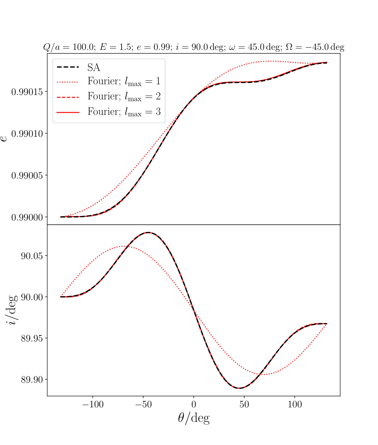 Figure 2
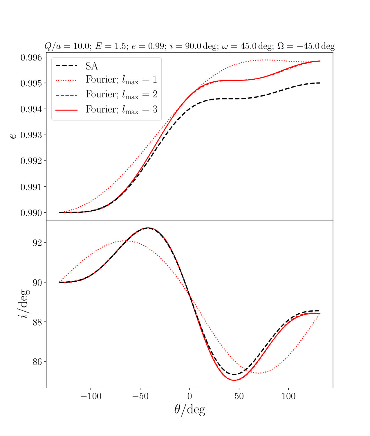 Figure 2
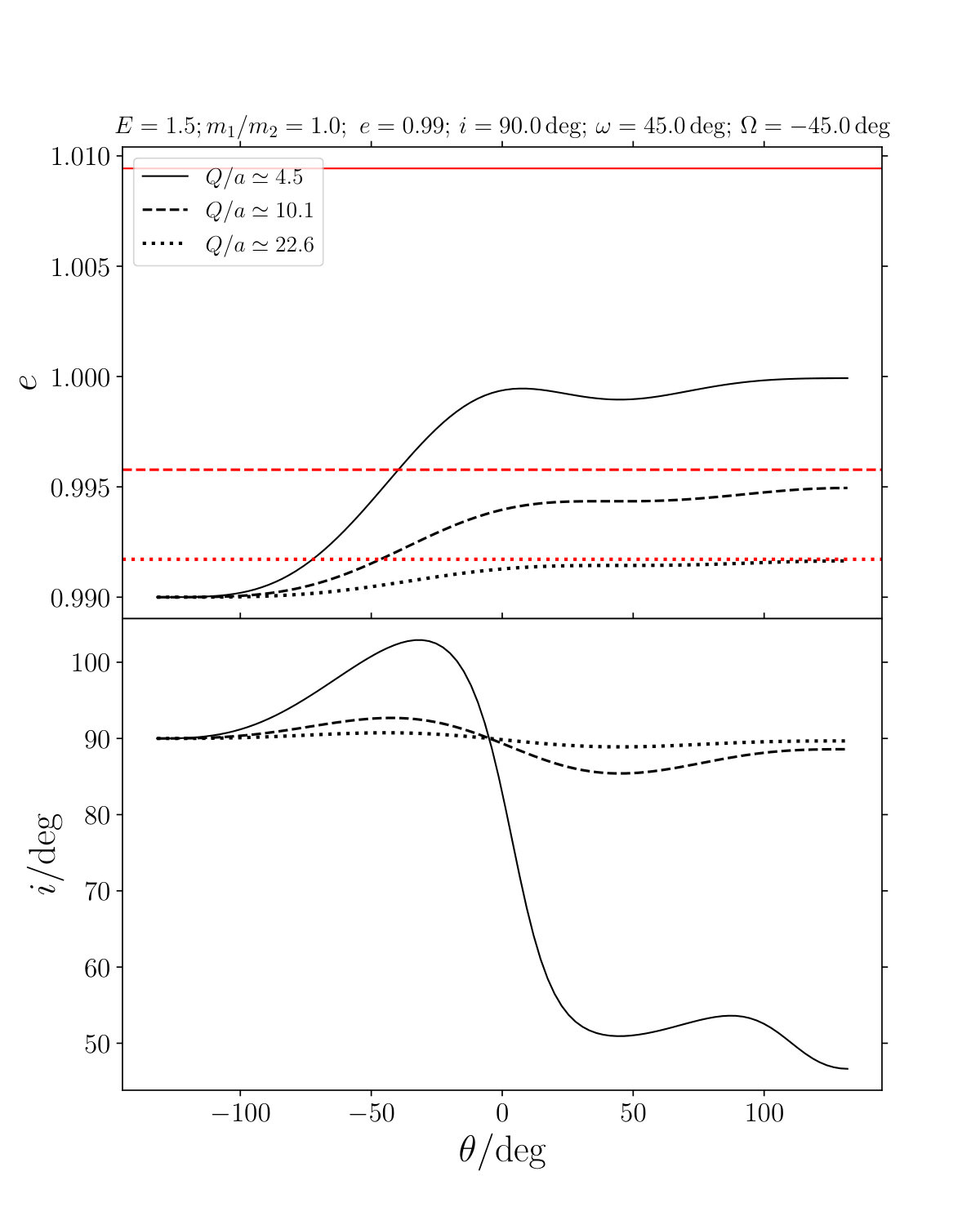 Figure 3
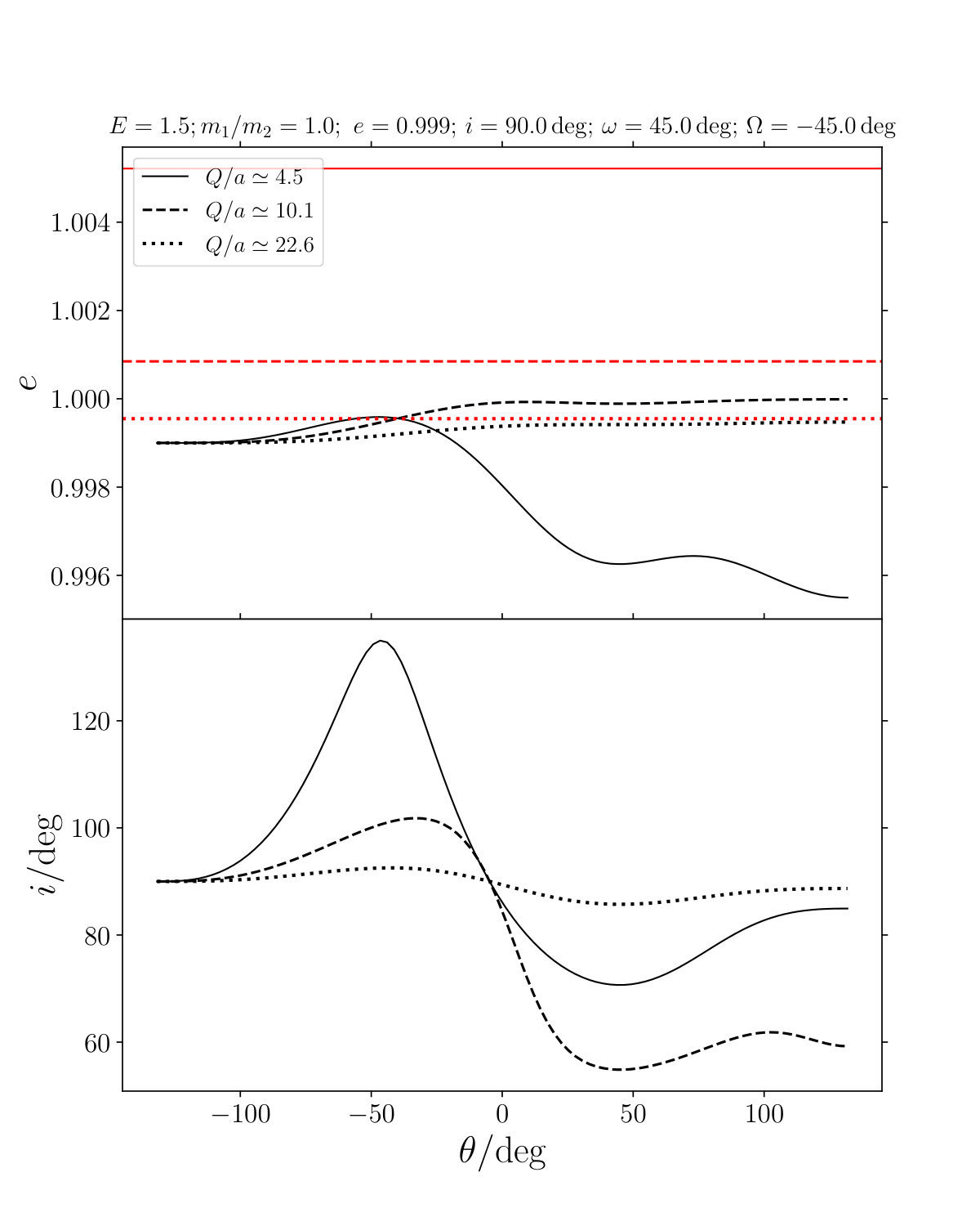 Figure 3
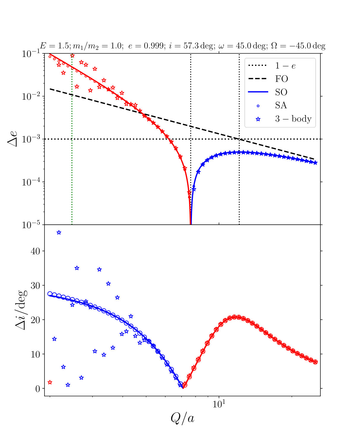 Figure 4
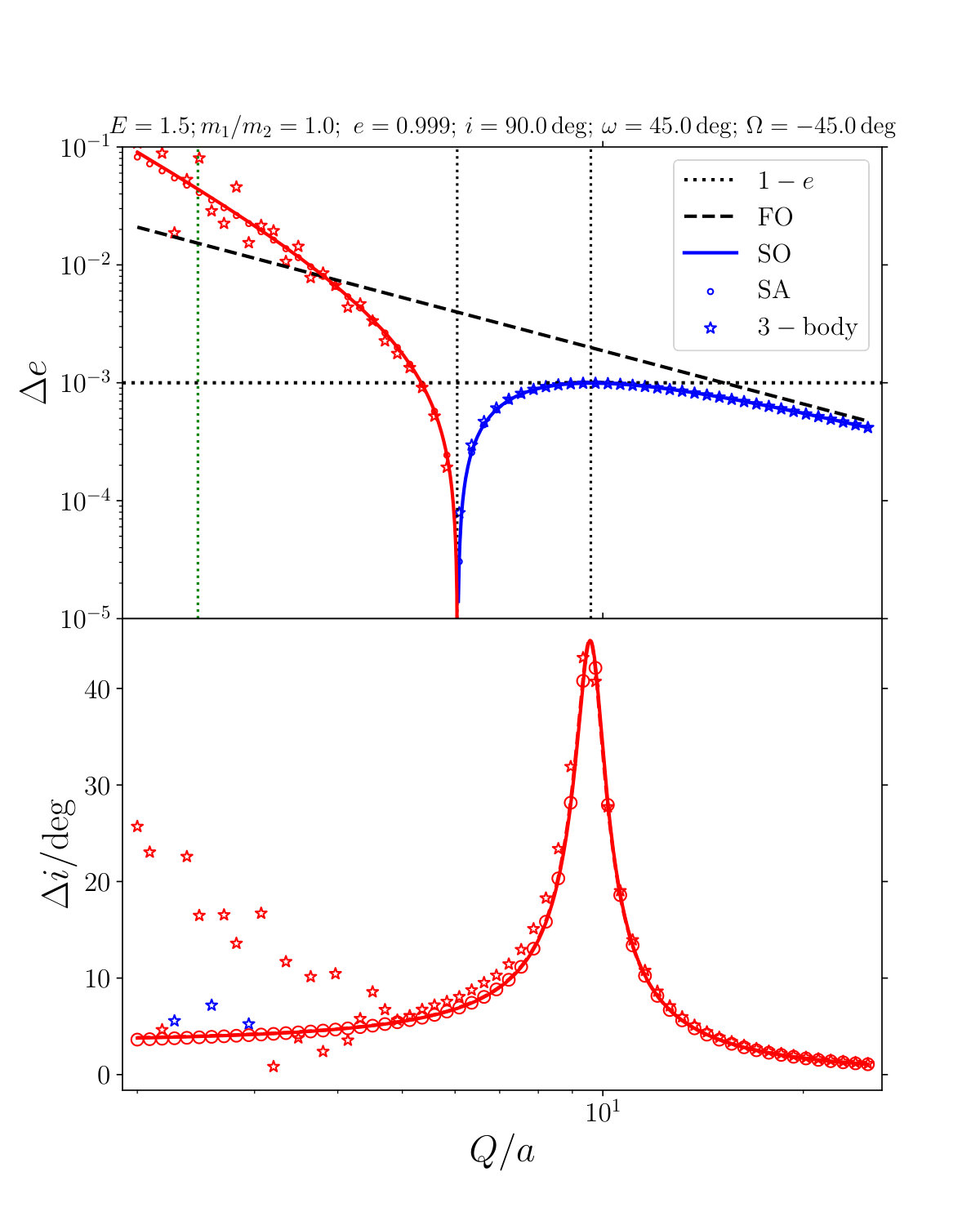 Figure 4
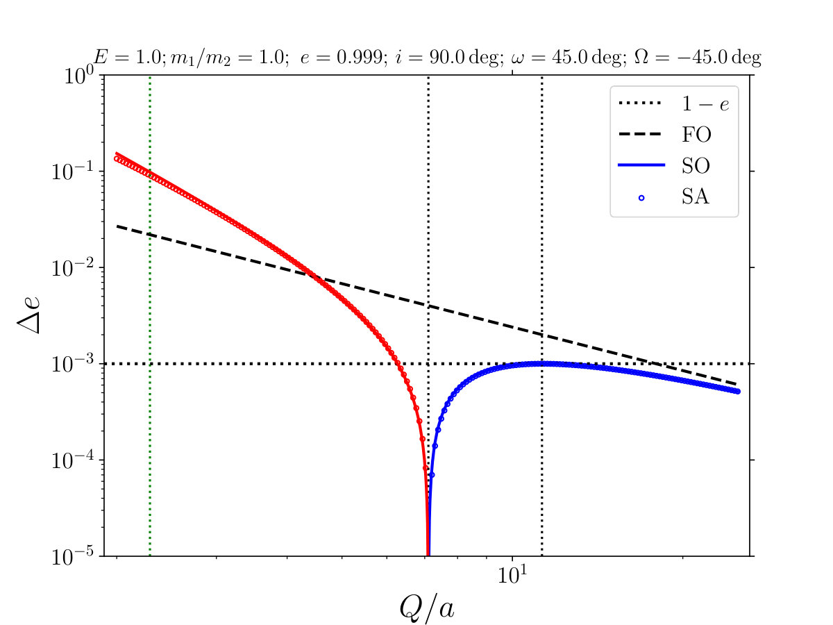 Figure 5
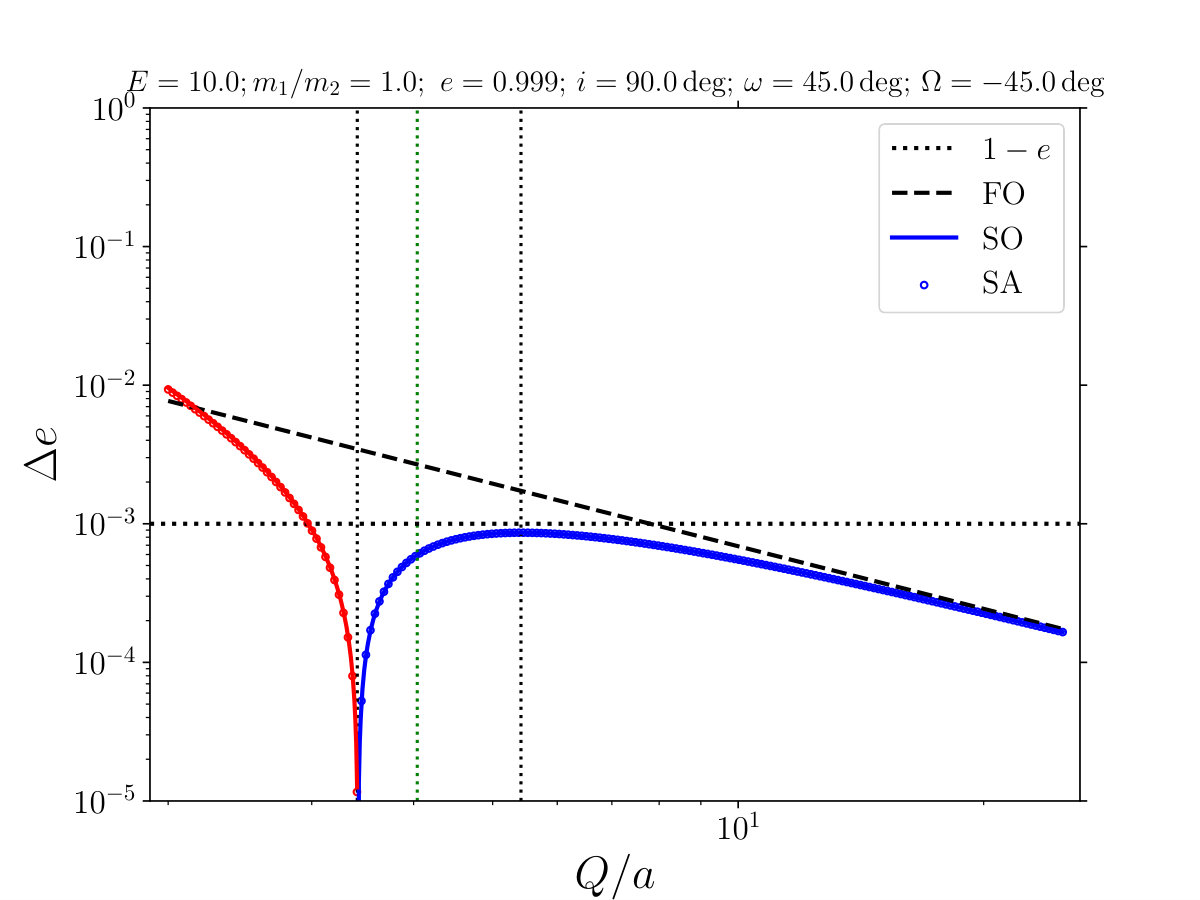 Figure 5
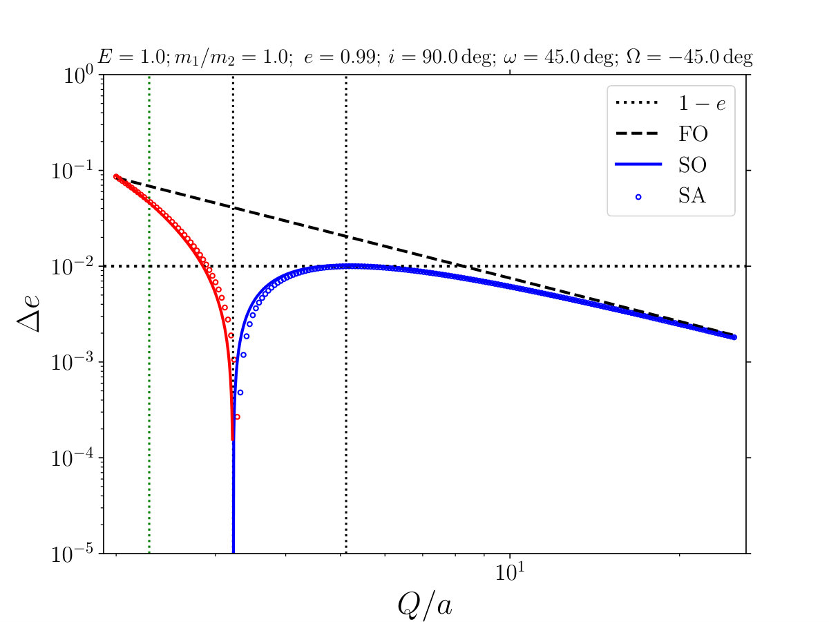 Figure 5
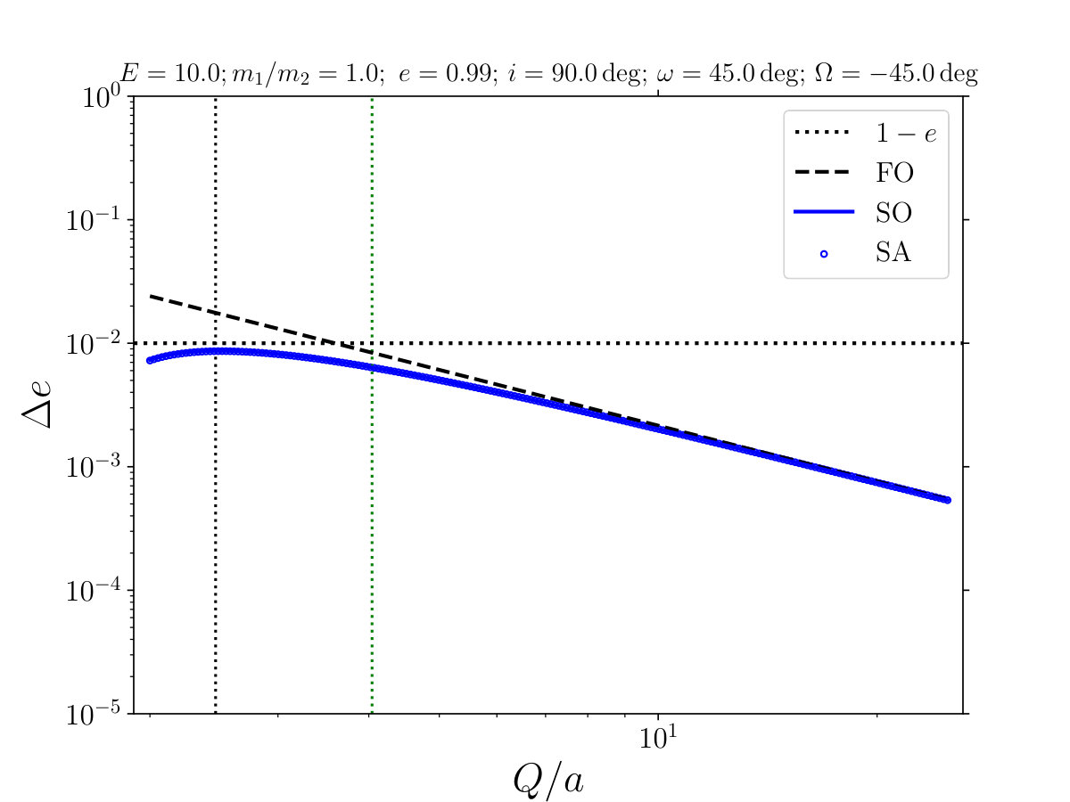 Figure 5
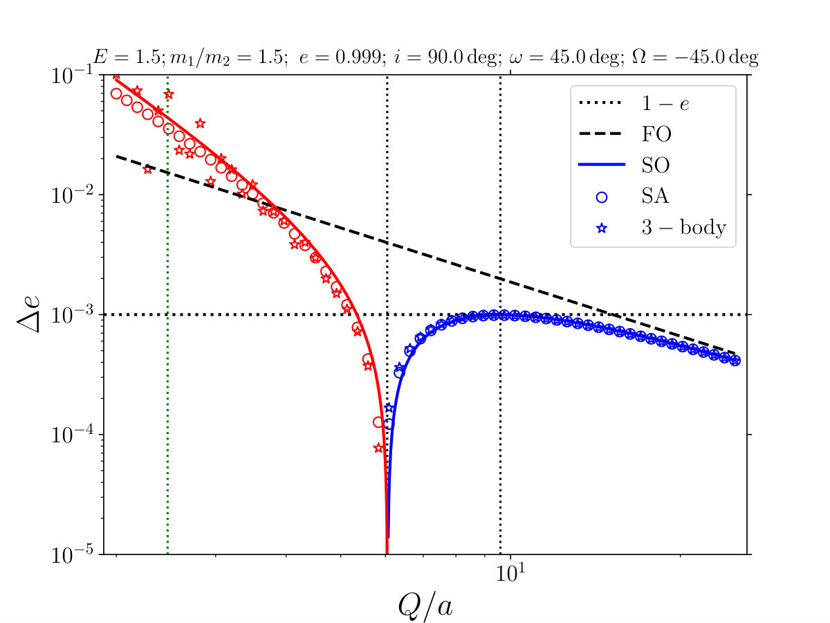 Figure 6
 Figure 6
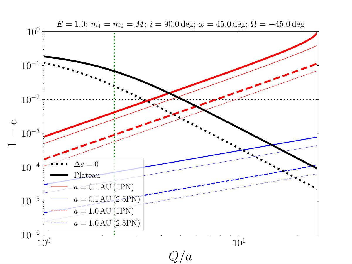 Figure 7
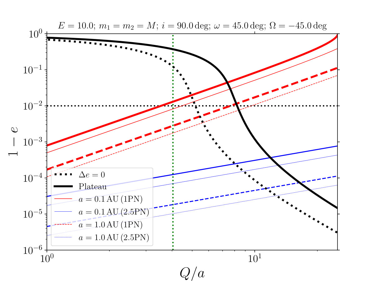 Figure 7
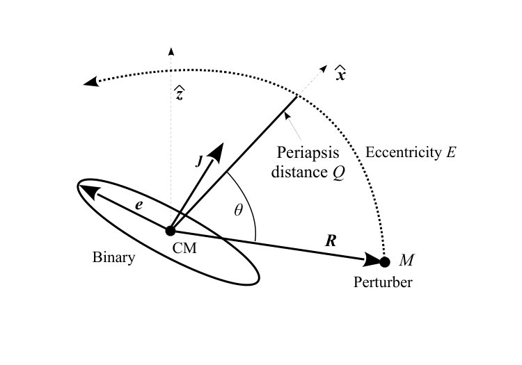 Figure 15
Peer Reviews
No public reviews on file for this paper yet. If you reviewed it on a platform where reviews are public (OpenReview, ICLR, NeurIPS, ICML), you can paste yours below so the community can read it here.
Videos
No videos yet. Explain this paper in a talk, walkthrough, or lecture? Add one.
Analytic computation of the secular effects of encounters on a binary: features arising from second-order perturbation theory
Adrian S. Hamers1 and Johan Samsing2
1Institute for Advanced Study, School of Natural Sciences, Einstein Drive, Princeton, NJ 08540, USA
2Department of Astrophysical Sciences, Princeton University, Peyton Hall, 4 Ivy Lane, Princeton, NJ 08544, USA E-mail: [email protected]: [email protected]
(Accepted 2019 June 9. Received 2019 June 4; in original form 2019 April 24)
Abstract
Binary-single interactions play a crucial role in the evolution of dense stellar systems such as globular clusters. In addition, they are believed to drive black hole (BH) binary mergers in these systems. A subset of binary-single interactions are secular encounters, for which the third body approaches the binary on a relatively wide orbit, and such that it is justified to average the equations of motion over the binary’s orbital phase. Previous works used first-order perturbation theory to compute the effects of such secular encounters on the binary. However, this approach can break down for highly eccentric binaries, which are important for BH binary mergers and gravitational wave sources. Here, we present an analytic computation using second-order perturbation techniques, valid to the quadrupole-order approximation. In our calculation, we take into account the instantaneous back-reaction of the binary to the third body, and compute corrections to previous first-order results. Using singly-averaged and direct 3-body integrations, we demonstrate the validity of our expressions. In particular, we show that the eccentricity change for highly eccentric binaries can reach a plateau, associated with a large inclination change, and can even reverse sign. These effects are not captured by previous first-order results. We provide a simple script to conveniently evaluate our analytic expressions, including routines for numerical integration and verification.
keywords:
gravitation – celestial mechanics – stars: kinematics and dynamics – globular clusters: general – stars: black holes
††pubyear: 2019††pagerange: Analytic computation of the secular effects of encounters on a binary: features arising from second-order perturbation theory–A.2
1 Introduction
There exists a large variety of astrophysical settings in which a binary system is perturbed by a passing object in a wider orbit. In the planetary context, stellar flybys can drive wide binaries to high eccentricities, leading to strong tidal interactions and/or stellar collisions (Kaib & Raymond, 2014), or destabilizing planetary systems (Kaib et al., 2013). In the Solar system, stellar encounters play an important role in disturbing the Oort cloud, thus transporting comets into the inner Solar system (Oort 1950, and, e.g, Heisler et al. 1987; Duncan et al. 1987; Dybczyński 2002; Serafin & Grothues 2002; Fouchard et al. 2011; Higuchi & Kokubo 2015). Such perturbations may also be responsible for triggering white dwarf pollution in extra-solar systems (e.g., Veras et al. 2014). In the stellar context, flybys may be important for producing low-mass X-ray binaries (Michaely & Perets, 2016), or gravitational wave sources (Michaely & Perets, 2019).
In dense stellar systems, flybys in which the binary remains bound after the encounter without exchanges can be considered a sub-type of more general binary-single interactions (e.g., Hut & Bahcall 1983; Hut 1983; Heggie & Sweatman 1991). Such interactions are key to driving the late-stage evolution of dense stellar systems such as globular clusters (e.g., Spitzer 1987; Binney & Tremaine 2008).
If the perturber passes the binary with a periapsis distance that is significantly larger than the binary semimajor axis, then the encounter is typically ‘secular’, i.e., the motion of the perturber is much slower than the orbital motion of the binary. In this case, it is appropriate to expand the Hamiltonian in terms of the ratio of the binary separation to the separation of the perturber to the binary center of mass, and to average the Hamiltonian over the binary motion. These procedures result in the simpler ‘singly-averaged’ (SA) equations of motion, which are computationally less intensive to solve compared to direct 3-body integrations. However, it is still necessary to numerically solve a set of first-order ordinary differential equations (ODEs) in order to obtain the new binary properties after the perturber’s passage.
It is also possible to apply first-order perturbation techniques, i.e., to analytically integrate the SA equations of motion assuming the perturber moves on a hyperbolic or parabolic trajectory, and ignoring changes of the binary’s orbital elements during the perturber’s passage. This approach was adopted in previous works (e.g., Heggie 1975; Heggie & Rasio 1996; Hamers 2018). In particular, the equations derived by Heggie & Rasio (1996) are commonly used to take into account the effects of (distant) encounters on a binary in Monte Carlo-style computations (e.g., Rasio & Heggie 1995; Spurzem et al. 2009; Geller et al. 2019).
However, there are situations in which the first-order perturbation approach can break down. In Heggie & Rasio (1996), it was discussed that their method no longer applies if the eccentricity change is of the order of the initial eccentricity, i.e., . However, as we will show here, when the binary is already highly eccentric, then the first-order approach can break down even if is small, in particular, if . The latter can occur in highly eccentricity binaries perturbed by distant (i.e., weak) encounters, which can drive relatively large changes in the binary’s orbital angular momentum. A binary can be driven to high eccentricities as a result of strong (non-secular) encounters in dense stellar systems. The breakdown of the first-order method originates from the fact that the binary’s elements can change significantly during the passage of the perturber. Therefore, it is not justified to assume that these elements are constant when integrating the equations of motion.
In this paper, we present an analytic computation of the change of the binary’s properties in the secular regime using second-order perturbation theory. In short, a Fourier expansion is used to describe the binary’s instantaneous response to the perturber, and this response is substituted back into the equations of motion in order to obtain correction terms to the first-order result. This approach is similar to that by Luo et al. (2016) applied to hierarchical triples (i.e., with a bound third object instead of an unbound one). In triples, similar interactions on the timescale of the third body can modulate the long-term secular interactions (e.g., Brown 1936; Ćuk & Burns 2004; Ivanov et al. 2005; Katz & Dong 2012; Antonini & Perets 2012; Seto 2013; Antognini et al. 2014; Bode & Wegg 2014; Lei et al. 2018; Grishin et al. 2018b). The correction terms give rise to behavior such as orbital flips and sign reversals in the eccentricity change that are not captured by first-order theory.
In an accompanying paper (Samsing et al., 2019), we investigate the astrophysical implications of secular encounters on highly eccentric binaries, for which the first-order perturbation approach can break down. In particular, the properties of black hole (BH) binary mergers and their subsequent gravitational wave (GW) signals are discussed.
This paper is structured as follows. We give an overview of previous results in Section 2. In Section 3, we apply second-order perturbation techniques, and derive analytic expressions for the changes of the binary’s properties in response to secular encounters. These results, which are summarized (for the case of parabolic encounters) in equation (3.2.2), can be interpreted as additions to the work of Heggie & Rasio (1996). In Section 4, we provide a simple Python script to conveniently evaluate our analytic expressions, illustrate the regime in which the first-order approximation breaks down, and demonstrate the correctness of our second-order results using numerically-obtained SA solutions, and direct 3-body integrations. We discuss our results in Section 5, and conclude in Section 6.
2 Previous results
2.1 Preliminaries
Consider a binary with semimajor axis and eccentricity ; the component masses are denoted as and , with the total binary mass . The instantaneous eccentricity or Laplace-Runge-Lenz vector is given by , where is the relative separation between the components, dots denote derivatives with respect to time, and hats denote unit vectors. The normalized angular-momentum vector is , with magnitude . Apart from the orbital phase, the binary state is completely described in terms of and (note that the six degrees of freedom in these two vectors reduce to effectively four, since , and – together with the orbital phase, the binary’s state is described by five quantities).
We assume that the binary is perturbed by a third body with mass , passing by on a parabolic or hyperbolic orbit with periapsis distance , and separation relative to the binary center of mass. In the case of a parabolic (hyperbolic) orbit, the perturber orbit’s eccentricity is (). Without loss of generality, we set the angular-momentum vector of the perturber’s orbit to be aligned with the -axis, and the eccentricity vector along the -axis (i.e., the periapsis of the perturber’s orbit points along the -axis). A sketch of the configuration is shown in Fig. 1.
We also assume that the perturber moves sufficiently slowly such that the ‘secular’ approximation applies, i.e., the mean motion of the binary is much faster than the perturber’s angular speed at periapsis. This condition can be written as (e.g., Hamers 2018; Liu & Lai 2018)
[TABLE]
This condition typically implies that the binary is ‘hard’, i.e., its orbital energy is much larger than the typical kinetic energy of perturbers (Heggie, 1975). More quantitatively, the ‘hardness’ of a binary in a cluster with velocity dispersion can be defined as , i.e., the ratio between the (absolute value of the) specific binding energy, and the typical perturber kinetic energy. Writing , this implies that and are related according to
[TABLE]
Therefore, if the binary is hard, , and
[TABLE]
Unless and/or , this implies that , i.e., a secular encounter.
Some of the results below are presented in terms of the binary’s orbital elements , in addition to the orbital vectors and . We define the inclination , argument of periapsis , and longitude of the ascending node in the usual way, i.e., the relation between the orbital angles and orbital vectors is
[TABLE]
We emphasize that our definition of the orbital elements differs from that of Heggie & Rasio (1996). The latter authors chose the binary orientation to be fixed, and used orbital elements to describe the orientation of the third body’s orbit. In contrast, we fix the orientation of the third body’s orbit, and use orbital vectors/elements to describe the binary’s orientation. In practice, this implies , , and , where elements with the subscript HR96 refer to Heggie & Rasio (1996), and elements without subscripts refer to the elements adopted here.
2.2 Equations of motion
We expand the Hamiltonian of the 3-body system in terms of the ratio of the separation of the binary, , to the separation of the third body relative to the binary center of mass, . To lowest order in , i.e., (quadrupole order), and after averaging over the binary mean motion assuming a Kepler orbit, the equations of motion for the binary orbital elements read (e.g., Hamers 2018)
[TABLE]
Here, is the true anomaly of the perturber’s (parabolic or hyperbolic) orbit, and the small parameter
[TABLE]
Generally, , where
[TABLE]
Assuming that lies in the -plane, we can write whereas for the binary, and . Therefore, equations (5) can be written in the explicit form
[TABLE]
We will refer to equations (5) and (8) as the SA equations of motion: averaged over the binary, but still explicitly a function of the perturber’s orbital phase .
2.3 First-order equations
The SA equations of motion constitute a system of ODEs and can be solved numerically. In addition, as in previous works (Heggie & Rasio 1996; Hamers 2018), the SA equations can be integrated over time from minus to plus infinity, or equivalently, over with , to obtain the changes in and . In the first-order (FO) approximation, the orbital vectors are assumed to be constant during the integration, i.e.,
[TABLE]
In equations (9), the integrands are evaluated at the initial values of the eccentricity and angular-momentum vectors, and the latter are assumed to be constant throughout the perturber’s passage (the components of and in the explicit expressions in equations 9 should be interpreted as the components of the initial vectors; for brevity, we omitted the subscript ‘0’). In other words, in the FO approximation, the binary is not allowed to respond to the instantaneous perturbation of the third body.
In the limit when the change in the eccentricity vector is small, equation (9) yields the following more manageable expression for the scalar eccentricity change,
[TABLE]
It can be shown that equation (10) is equivalent to the quadrupole-order result of Heggie & Rasio (1996; see also Appendix A2.2 of Hamers 2018).
3 Analytic second-order computation
The FO approximation works well in the limit when the changes in the binary’s state are small. However, in some cases, the change in and can be significant compared to the initial values (for example, when the initial eccentricity is already very high). In this case, it is no longer justified to assume that and are constant as in equations (9), i.e., FO perturbation theory is insufficient (see also Hamers 2018).
To derive improved expressions, we adopt a similar approach as Luo et al. (2016). In short, we develop Fourier expansions of the SA equations of motion. The orbital vectors, , are also written in the form of Fourier expansions. By plugging the Fourier expansions of and into the equations of motion, we obtain explicit relations for the Fourier coefficients associated with and . Subsequently, we integrate the equations of motion, now taking into account the leading order Fourier coefficients. The result consists of the original FO term, plus new additional terms to second order (SO). In other words, using Fourier expansions, we compute the instantaneous response of the binary to the perturber, and use the updated expressions to more accurately calculate the net effects on the binary elements.
3.1 Fourier expansions of the SA equations of motion
3.1.1 Calculation
First, we develop the Fourier series expansions of equations (8), i.e.,
[TABLE]
with the Fourier coefficients given by
[TABLE]
Here, the SA equations of motion in the integrands are to be evaluated at constant and (i.e., the initial values). Explicit expressions for these Fourier coefficients are given in Appendix A.1. Note that, trivially,
[TABLE]
The summations in equations (11) run from to . In the case of a bound third body (Luo et al., 2016), the Fourier coefficients vanish identically for . It turns out that, in our case of an unbound third body, the Fourier coefficients do not vanish for . In principle, an infinite number of terms should be included. However, in practice, it suffices to restrict to a finite . In our explicit expressions, we set (see Section 3.1.2 below for the justification).
Next, we assume that the binary orbital vectors can be written in terms of similar Fourier series but with the addition of a linear term, i.e.,
[TABLE]
Here, , , and are constant vectors, and the Fourier coefficients , , and associated with and are understood to be functions of the initial values of and . We substitute equations (15) into equations (11) by differentiating the former with respect to . Subsequently, we equate the coefficients of all terms (constant terms, and the sine and cosine terms) on both sides of the resulting equality. This procedure gives the following relations between the coefficients of the orbital vectors, and , and those of the equations of motion,
[TABLE]
The necessity of the linear terms in equations (15) becomes clear by noting that without them, the -derivatives of equations (15) would not contain a term independent of , whereas such a term is present in equations (11). We remark that the linear term was omitted in Luo et al. (2016).
Equations (15) describe the instantaneous response of the binary to the perturber in terms of an infinite Fourier series. They can be written in the more compact form
[TABLE]
Here, and are the initial state vectors, and and are (known) functions of , defined by
[TABLE]
3.1.2 Testing the Fourier expansions
To demonstrate the correctness and usefulness of the Fourier expansions, we show in Fig. 2 the eccentricity and inclination of a binary perturbed by a third body as a function of the third body’s orbital phase . We set , , , , , and . In the left (right)-hand panels, (), corresponding to (). The black solid lines show and obtained by numerically integrating the SA equations of motion, i.e., equations (8). Within the limit of the SA and quadrupole-order approximation, these solutions can be considered to be exact. Red lines correspond to the Fourier series in equations (17), where we take to be either 1, 2 or 3.
In the case of , the Fourier series accurately describe and , provided that . There are no noticeable differences between and . For (i.e., larger ), the Fourier series still give a reasonable approximation of the true and , although there are significant differences, in particular for . The discrepancy in the case between the numerical solutions and the Fourier series can be traced to the fact that we included terms of order in equations (17), and ignored terms of order . Evidently, higher-order terms become increasingly important as increases. Note that convergence with respect to is distinct from convergence with respect to . In the case of , the series in still converges for .
3.2 Calculating corrections to second order in
3.2.1 General case: hyperbolic orbits
The next step is to substitute and up to and including first order in into the equations of motion, equations (11), where the Fourier coefficients , , , , , and are now all evaluated using equations (17), and subsequently integrating over from to .
To first order in , this procedure simply yields
[TABLE]
i.e., we recover the FO result (note that, to zeroth order in , , and similarly for the sine terms and the other Fourier coefficients). For future convenience, we defined the two functions
[TABLE]
To second order in , the general result is (much) more complicated. Specifically,
[TABLE]
Here, and , which are composed of and respectively, are known functions of , , and . The functions and are easily obtained through
[TABLE]
Here, and are the -independent terms of equations (17), i.e.,
[TABLE]
In other words, and can be obtained by taking the FO result (i.e., and for the eccentricity and angular-momentum vector, respectively), and replacing the initial state vectors with and given by equations (23). Note that this result is independent of the value of . The explicit substitution relations in equations (23) are given in Appendix A.2. The functions and do depend on the assumed value of , and are generally very complicated. We therefore do not give the explicit expressions for and here. Instead, we implemented all required functions in an easy-to-use script that is freely available and described below (see Section 4).
In compact notation, the SO result can be written as
[TABLE]
In the limit of small changes, the scalar eccentricity change to second order in is given by
[TABLE]
Generally, the inclination change is given by
[TABLE]
3.2.2 The parabolic limit
In the parabolic limit (), the SO expressions become much less complicated. Specifically,
[TABLE]
The above expressions imply that, in the limit of small changes and parabolic orbits, the scalar eccentricity change is given by
[TABLE]
In equation (3.2.2), we also wrote the result in terms of the orbital elements. It can be shown that equation (3.2.2) is consistent to order with equation (8) of Heggie & Rasio (1996), using that and , together with evaluated at (cf. equation 6). The novel result of this paper is the SO term in equation (3.2.2).
4 Exemplifying the correctness and relevance of the second-order expressions
In this section, we illustrate interesting behavior in the limit of high binary eccentricities, in which case the analytic FO expressions for the scalar eccentricity change can break down and a SO calculation is warranted. We demonstrate the correctness of our SO expressions by comparing to results obtained by numerically integrating the SA equations, and by directly integrating the 3-body equations of motion (i.e., without averaging over the binary’s motion).
We freely provide111https://github.com/hamers/flybys a simple Python script to compute the FO and SO expressions. In this script, which requires only the numpy and scipy libraries, we also include functionality to integrate the SA equations of motion numerically, and to carry out direct 3-body integration. The script can be used to quickly generate all the figures presented in this paper.
4.1 Phase evolution
In Fig. 3, we show the binary eccentricity and inclination as a function of the perturber’s true anomaly assuming , , , , and . In the left (right)-hand panels, (. In each panel, three values of are chosen, ranging from relatively large, (), to small (). These results were obtained by numerically integrating the SA equations of motion. The red horizontal lines show according to FO perturbation theory (equation 10).
We first consider the case when the initial binary eccentricity is (left-hand panel in Fig. 3). For relatively large , , the changes in eccentricity and inclination are small. The FO equation accurately describes the scalar eccentricity change. However, as decreases, the agreement worsens, and for , the FO equation even yields , which is clearly not physical (note that, according to both SA and direct integration, the binary remains bound with a high eccentricity).
In the right-hand panel of Fig. 3, the initial binary eccentricity is even higher, (all other parameters are the same as in the left-hand panel). As shown with the SA integrations, as decreases, the maximum eccentricity reached during the perturber’s passage increases. This continues until, at a critical value of , the maximum eccentricity reached during the passage approaches unity, and the binary subsequently ‘bounces back’ to lower eccentricity. Consequently, the net scalar eccentricity change becomes negative. This phenomenon is also associated with a large change in the inclination, and is similar to the flipping of orbits associated with very high eccentricities in hierarchical systems such as triples (e.g., Lithwick & Naoz 2011; Grishin et al. 2018b), and higher-order systems (e.g., Hamers & Lai 2017; Grishin et al. 2018a). The FO equation fails to describe this ‘bounce’ effect, and incorrectly predicts a net increase of the eccentricity, and which is .
4.2 Series of
4.2.1 General behavior
As described above, for high initial binary eccentricities and assuming that for weak perturbations the binary’s eccentricity is increased, for sufficiently strong perturbations (small ), the binary eccentricity shows a ‘bounce’ phenomenon, resulting in a net negative scalar eccentricity change. Here, we describe this effect more quantitatively and show that our SO results can be used to accurately describe the binary’s eccentricity and angular-momentum changes in the associated parameter space.
In Fig. 4, we show the scalar eccentricity change and inclination in the top and bottom panels, respectively, as a function of . The fixed parameters are , , , , and . In the left (right)-hand panels, the binary’s inclination is (). We show analytic FO results (black dashed lines), analytic SO results (colored solid lines), numerical SA results (colored open circles), and 3-body integration results (colored stars). Blue (red) colors correspond to positive (negative) changes.
The 3-body integrations were carried out by formulating the 3-body equations of motion into ODE form and solving this set of equations using the odeint routine from the Python package scipy. This routine is based on the LSODA Fortran integrator, which uses variable time steps to integrate the system of ODEs. LSODA automatically and dynamically switches between stiff and nonstiff methods; for stiff cases, it uses the backward differentiation formula method (with a dense or banded Jacobian), and for nonstiff cases it uses the Adams method. Error control within the solver is determined by the input parameters rtol and atol, such that the error in each ODE variable is less than or equal to . We set the relative and absolute tolerance parameters to and , respectively. Typical relative energy errors were (for small , corresponding to few binary orbits), to (for large , corresponding to many binary orbits).
We first describe the behavior shown in Fig. 4 according to the SA and 3-body integrations. For large , the SA and 3-body integrations agree well. As stated above, the 3-body energy errors are largest for large , but the good agreement with the SA results indicates that the 3-body integrations can still be trusted. As decreases, starts to flatten, and reaches a local maximum, at . This plateau in is associated with a large inclination change (see the bottom panels in Fig. 4). In the case when , the plateau corresponds to , the maximum allowed positive change (shown with the black horizontal dotted lines).
For smaller , decreases with increasing , and at a critical value of , , changes sign. Subsequently, increases, with a different slope compared to before the sign change (in fact, this slope is , as shown below in Section 4.2.2). At small , , the SA and 3-body results start to differ significantly. This is the result of the breakdown of the SA approximation: for very small ( approaching unity), the binary’s motion is no longer much faster than the perturber’s motion, therefore it is no longer justified to average over the binary motion. This is also supported by the green vertical dotted line, which shows the value of for which (see equation 1). The scatter in the 3-body results originates from the binary phase-dependence in this regime (we assumed a fixed initial binary phase of ).
The FO expression gives a good description at large , but clearly fails as . The SO results, shown with the solid colored lines, agree well with the SA results for any and, therefore, with the 3-body results, unless .
In Fig. 5, we show similar results for different parameter choices in four panels with (parabolic encounter) or , and or . The SO expression generally gives a good description. Some deviation can be seen in the case when and , which can be attributed to higher-order terms in (i.e., ) that are important for small . Higher-order terms are left for future work.
4.2.2 Useful properties of the SO solution
Evidently, the SO solution removes the need for numerical integration of the equations of motion. The latter can be achieved with the SA approximation, or with the most general but also most computationally expensive method of direct 3-body integration. The implied speed-up can be advantageous when a large number of encounters need to be evaluated, e.g., in Monte Carlo approaches.
In addition, the SO equations can be used to gain more insight into the effect of secular encounters. In the case of the series of discussed in the previous section, the value of (corresponding to a particular ) for the sign change of can be simply expressed using equation (25), i.e.,
[TABLE]
The value of corresponding to the plateau (, or, equivalently, ) is easily found to be
[TABLE]
In terms of (see equation 6), the latter implies
[TABLE]
In Figs 4 and 5, we show in each -panel with the two vertical black dotted lines the values of corresponding to the sign change and plateau according to equations (29) and (30).
Although the expression in equation (29) seems simple, the explicit relation in terms of , and is very complicated (this can be mainly attributed to the complicated function ). Fortunately, in the limit of parabolic orbits, greatly simplifies (see Section 3.2.2); in this case, reduces to
[TABLE]
Another property that immediately follows from the SO solution is the slope in the small regime in which is negative. In the small regime, the term in equation 25) dominates. Therefore, , which is consistent with the numerical results.
5 Discussion
5.1 Higher-order expansion terms
Our derivation of the SO corrections were based on the quadrupole-order SA equations of motion, equations (5). However, for small , higher-order terms in the Hamiltonian expansion in terms of are generally also important. In particular, the next-order terms in the Hamiltonian are the octupole-order terms (), which give rise to terms in the SA equations of motion given by (e.g., Hamers 2018)
[TABLE]
Here, the ‘octupole parameter’ (analogous to the octupole parameter in hierarchical triples, e.g., Lithwick & Naoz 2011; Katz et al. 2011; Teyssandier et al. 2013; Li et al. 2014, or more generally in hierarchical systems, Hamers & Portegies Zwart 2016) is defined by
[TABLE]
In the examples in Section 4, we chose implying that the octupole-order terms vanish; the quadrupole-order SO results generally agreed with the 3-body integrations. However, for unequal masses of the binary components, the octupole-order terms do not vanish, and can give significant contributions for small . This is illustrated in Fig. 6, in which, similarly to Fig. 4 but here for unequal binary mass component cases, is plotted as a function of . In the case of the SA integrations, the octupole-order terms (equations 33) were included. The ‘SO’ lines include the FO octupole-order prediction, which can be obtained by integrating equations (33) assuming constant and , yielding a scalar eccentricity change given by
[TABLE]
In the left-hand panel, we set and ; in the right-hand panel, and . The perturber mass in both cases is .
Fig. 6 shows that our SO prediction with the inclusion of the FO octupole-order terms does not accurately describe , particularly as the difference increases. The octupole-order SA equations still give good agreement with the 3-body integrations, provided that (otherwise, the SA approximation breaks down).
This discrepancy can be understood by noting that the octupole-order equations of motion give rise to additional terms in the Fourier expansion of and , equations (15), of order (and higher orders). Consequently, the lowest-order contribution from the SO octupole-order term will be of the order of (and not , as might be naively expected).
A derivation of the SO octupole-order terms is beyond the scope of this paper, and is left for future work.
5.2 Third body’s orbit
In our calculations, we assumed that the perturber’s orbit is perfectly hyperbolic or parabolic. In reality, as the perturber’s orbit becomes less secular (in particular, for smaller ), deviations from hyperbolic or parabolic orbits may become increasingly important. Analytic calculations taking into account such deviations are beyond the scope of this work. However, such corrections may not even be useful, since the SA approximation typically breaks down in similar regimes as (equation 1) approaches unity.
5.3 Applicability to star clusters
We assumed that the (dynamical) effects of other stars on the evolution of a binary in a star cluster can be described in terms of a restricted problem in which a single perturber approaches the binary on a parabolic or hyperbolic orbit. Reality is, of course, more complicated. For example, due to perturbations from other stars, the orbit of the third body relative to the binary is never exactly parabolic or hyperbolic. However, the effect of the third body on the binary is highly concentrated near periapsis, since . Therefore, we expect that the exact shape of the orbit at larger distances from the binary is not very important for the evolution of the binary. Also, in a real system, the cluster potential (i.e., other stars viewed as a whole) can affect the binary, depending on the potential properties (see, e.g., Hamilton & Rafikov 2019a, b).
Another related point of concern is that not all encounters are safely in the secular regime, which we assumed here. The fraction of secular encounters can be crudely estimated as , where is the critical impact parameter delineating secular from nonsecular encounters222Of course, in reality there is no sharp boundary between secular and non-secular encounters., and is the largest impact parameter considered. For the typical parameters assumed in this paper, (see, e.g., the vertical green dotted lines in Figs 4, 5, and 6), implying a fraction of secular encounters for given given by . If is taken to be , a tenth of the typical core radius of a globular cluster and roughly the typical size of dense subclusters of BHs formed in globular clusters (e.g., Banerjee et al. 2010), then the fraction of secular encounters for a binary with a semimajor axis of is . Clearly, most encounters are secular. Evidently, although non-secular encounters are rare, they can dramatically affect the binary. The combined effect of strong and weak encounters is discussed in Samsing et al. (2019).
5.4 Overview of parameter space
We showed that the (scalar) eccentricity change due to secular encounters can significantly deviate from the analytic prediction of Heggie & Rasio (1996) when the initial binary eccentricity is high. Using our analytic SO expressions, we here quantify the parameter space in which this deviation is important, focusing on BH binaries in dense stellar clusters and also considering the importance of post-Newtonian (PN) terms.
In Fig. 7, we show, in the parameter space (where is the initial binary eccentricity), locations for which the sign change in occurs (dotted black lines), and for which reaches a plateau (solid black lines). Generally, these two values are given by equations (29) and (30), respectively (also note that there exists a general relation between the two as described by equation 31). Here, we set , , , ; the left (right)-hand panels correspond to (). For a given value of , the black lines indicate the initial eccentricity for which the sign change and plateau phenomena occur; above the black dashed line (smaller eccentricity), the result of Heggie & Rasio (1996; i.e., first order in ) is expected to give an at least reasonable description of , whereas below it, higher-order terms in (second order and higher) become important.
Generally, the initial binary eccentricities for which reaches a sign change or plateau increase with increasing . A larger initial implies that a smaller change in the binary eccentricity can push the binary towards unity eccentricity (which is associated with the sign change and plateau phenomena), implying a weaker perturbation and hence a larger value of . In the case of and a perturber with , a binary needs to have an initial eccentricity of for deviations from Heggie & Rasio (1996) to be important. For , the required eccentricity is . From equation (4.2.2), it follows that in the limit of parabolic orbits and high initial binary eccentricity, , i.e., , consistent with the high-eccentricity behaviour shown with the black lines in the left-hand panel in Fig. 7.
PN terms are potentially important for BH binaries in dense stellar systems. Here, we estimate the importance of the lowest-order PN terms, which are of the order of , where is the binary’s orbital speed and is the speed of light. The 1PN terms give rise to precession of the binary’s line of apsides at a rate given by (e.g., Weinberg 1972)
[TABLE]
Here, is the binary’s gravitational radius, and is the binary’s mean motion. Analogously to triple systems (e.g., Blaes et al. 2002; Wu & Murray 2003; Fabrycky & Tremaine 2007; Thompson 2011; Naoz et al. 2013; Liu et al. 2015) and orbits around a massive BH (e.g., Merritt et al. 2011; Brem et al. 2014; Hamers et al. 2014; Bar-Or & Alexander 2014, 2016; Bar-Or & Fouvry 2018), rapid relativistic precession can decrease the efficiency of the Newtonian torque exerted by the third body. To investigate the importance of the 1PN terms, it is therefore relevant to compare the relativistic rate, equation (36), to the (Newtonian) precession rate associated with the third body, . For simplicity, we evaluate the latter using the quadrupole-order term at periapsis of the perturber (), giving (see also equation 5)
[TABLE]
Here, , and depends on the binary orientation and is given by
[TABLE]
Setting gives the following relation for the binary eccentricity above which we expect 1PN terms to become important,
[TABLE]
Equation (39) is shown in Fig. 7 with the red lines, where solid (dashed) lines correspond to (, and thick (thin) lines correspond to (). Note that the 1PN terms break the scale-invariance of the problem, hence explicit values for the masses and the binary semimajor axis should be specified. For a given , 1PN terms are important for any initial binary eccentricity with (points below the red lines). For high eccentricities, equation (39) gives the scaling , consistent with Fig. 7. The red lines in Fig. 7 show that 1PN terms are potentially important for encounters with highly eccentric and tight binaries.
A higher order PN effect is the dissipation of orbital energy and angular momentum by GWs. The (lowest-order) associated PN term, the 2.5PN term, gives rise to an eccentricity decay rate given by (Peters, 1964)
[TABLE]
where after the approximation sign we assumed . The eccentricity change due to the third body, evaluated at and at the quadrupole order, is given by (see also equation 5)
[TABLE]
where
[TABLE]
The dissipative PN terms become important during the passage of the perturber if , i.e., when (in the limit of high binary eccentricity)
[TABLE]
Equation (43) is shown in Fig. 7 with the blue lines, where solid (dashed) lines correspond to (, and thick (thin) lines correspond to (). The scaling inferred from equation (43) is , consistent with Fig. 7.
Clearly, the dissipative PN terms are only important for binaries with extremely high eccentricity. However, such binaries are likely to merge rapidly due to GW emission before any encounter can change the binary’s properties. The latter is illustrated in Fig. 7 with the horizontal black dotted line, which shows the typical eccentricity for which, in a globular cluster, a BH binary is expected to merge due to GW emission before a next encounter (e.g., Samsing & D’Orazio 2018).
A caveat of the criterion equation (43) is that the dissipative term in equation (40) is evaluated at the initial binary eccentricity. In reality, the binary eccentricity changes during the encounter, potentially significantly reducing the merger time-scale (this issue will be addressed in future work, Samsing et al. 2019). A complete calculation of the SO terms with the inclusion of PN terms is beyond the scope of this paper.
6 Conclusions
We presented an analytic calculation of the secular effect on a binary of a perturber moving on a hyperbolic or parabolic orbit. We extended previous works (Heggie & Rasio, 1996; Hamers, 2018) in which first-order (FO) perturbation theory was used, by applying second-order (SO) perturbation techniques. Our results can be used to evaluate the importance of distant encounters on the evolution of eccentric binaries in dense stellar systems. The conclusions are given below.
-
In the FO approximation, the binary’s orbital elements are assumed to be constant during the passage of the third object. However, in some cases, particularly when the binary eccentricity is high (specifically, if ), the FO approximation can break down due to a relatively large change of the binary’s orbital elements during the passage. We used a Fourier series expansion to derive SO correction terms, which take into account the binary’s varying orbital elements. We derived explicit expressions for the change in the eccentricity and angular-momentum vectors of the binary, and , respectively, as a function of the initial parameters of the system.
-
The general SO expressions for and are very complicated. We provided a freely-available and simple Python script to evaluate them, including, for reference and testing purposes, routines to numerically integrate the singly-averaged (SA) equations of motion, and the non-averaged, direct 3-body equations of motion (see Section 4 for the url). In the limit of parabolic encounters (), the SO expressions become manageable, leading to a simple closed-form expression for the scalar eccentricity change (equation 3.2.2). The latter can be used to quickly explore the importance of the SO term (without a need to use our supplied Python script).
-
We tested the SO expressions for a number of cases with highly eccentric binaries. Such binaries are formed as a result of strong dynamical encounters in dense stellar systems. We showed that, as the perturber periapsis distance decreases, reaches a plateau, and subsequently drops and changes sign. For even smaller , increases with decreasing with a steeper slope compared to larger . We showed that our SO expressions accurately describe this phenomenon, in the limit when the octupole-order terms are unimportant (e.g., if ), and the secular approximation applies (i.e., it is justified to average over the binary’s motion). In contrast, the (quadrupole-order) FO expression from Heggie & Rasio (1996) predicts incorrect and unphysical eccentricities in this regime (in some cases, even ).
-
Our SO expressions were derived from the quadrupole-order equations of motion (i.e., obtained by an expansion of the Hamiltonian to second order in the separation of the binary to the separation of the third body relative to the binary’s center of mass). For small perturber periapsis distances, higher-order terms can be important. We briefly discussed these terms in Section 5.1, but a computation of the associated SO terms is left for future work.
-
We briefly explored the parameter space in which the plateau and sign change phenomena described above are important (see Section 5.4). We also showed that PN terms are potentially important for reducing the effect of secular encounters for highly eccentric (BH) binaries.
Acknowledgements
We thank Scott Tremaine for helpful discussion, and comments on the manuscript. We also thank Stephen McMillan and Piet Hut for stimulating discussions, Douglas Heggie, Fred Rasio, Evgeni Grishin, and Chris Hamilton for comments on the manuscript, and the anonymous referee for a helpful report. A.S.H. gratefully acknowledges support from the Institute for Advanced Study, and the Martin A. and Helen Chooljian Membership. J.S. acknowledges support from the Lyman Spitzer Fellowship.
Appendix A Explicit expressions
A.1 Fourier coefficients
Here, we give the explicit expressions for the Fourier coefficients of the equations of motion (with ), defined in equations (12).
[TABLE]
Here, is a function of and , given by
[TABLE]
A.2 Partial SO expressions
As mentioned in Section 3.2.1, the general (i.e., hyperbolic) expressions for and are excessively complicated, and are not given explicitly here (see Section 4 for an url to an easy-to-use script in which the general expressions for the eccentricity changes are implemented). Here, we give a partial hyperbolic result in the form of the functions and . As discussed in Section 3.2.1, these functions can be obtained from the FO result (i.e., and ) as described by equation (22), with the substitutions given by equation (23). The explicit expressions for these substitutions are given below.
[TABLE]
The reference list from the paper itself. Each links out to its DOI / PubMed record.
- 1Antognini et al. (2014) Antognini J. M., Shappee B. J., Thompson T. A., Amaro-Seoane P., 2014, MNRAS , 439, 1079 · doi ↗
- 2Antonini & Perets (2012) Antonini F., Perets H. B., 2012, Ap J , 757, 27 · doi ↗
- 3Banerjee et al. (2010) Banerjee S., Baumgardt H., Kroupa P., 2010, MNRAS , 402, 371 · doi ↗
- 4Bar-Or & Alexander (2014) Bar-Or B., Alexander T., 2014, Classical and Quantum Gravity , 31, 244003 · doi ↗
- 5Bar-Or & Alexander (2016) Bar-Or B., Alexander T., 2016, Ap J , 820, 129 · doi ↗
- 6Bar-Or & Fouvry (2018) Bar-Or B., Fouvry J.-B., 2018, Ap J , 860, L 23 · doi ↗
- 7Binney & Tremaine (2008) Binney J., Tremaine S., 2008, Galactic Dynamics: Second Edition. Princeton University Press
- 8Blaes et al. (2002) Blaes O., Lee M. H., Socrates A., 2002, Ap J , 578, 775 · doi ↗