On Detection of Critical Events in a Finite Forest using Randomly Deployed Wireless Sensors
Kaushlendra K. Pandey, Abhishek K. Gupta

TL;DR
This paper analyzes the effectiveness of randomly deployed wireless sensors in detecting critical, time-evolving forest events like wildfires, using a finite Boolean-Poisson model to derive sensing probabilities and coverage metrics.
Contribution
It introduces a finite Boolean-Poisson model for sensor deployment in forests and derives analytical expressions for event detection probabilities and sensing coverage.
Findings
Derived the distribution of contact distance in the model
Calculated the capacity functional of the sensor network
Formulated the probability of event detection over time
Abstract
Ecosystem of a forest suffers from many adverse events such as wild-fire which can occur randomly anywhere in the forest and grows in size with time. This paper aims to analyze performance of a network of randomly deployed wireless sensors for the early detection of these time-critical and time-evolving events in a forest. We consider that the forest lies in a confined space (e.g. a circular region) and the wireless sensors, with fixed sensing range, are deployed within the boundary of forest itself. The sensing area of the network is modeled as a finite Boolean-Poisson model. In this model, the locations of sensors are modeled as a finite homogeneous Poisson Point Process (PPP) and the sensing area of each sensor is assumed to be a finite set. This paper aims to answer questions about the proximity of a typical sensor from a randomly occurred event and the total sensing area covered by…
Click any figure to enlarge with its caption.
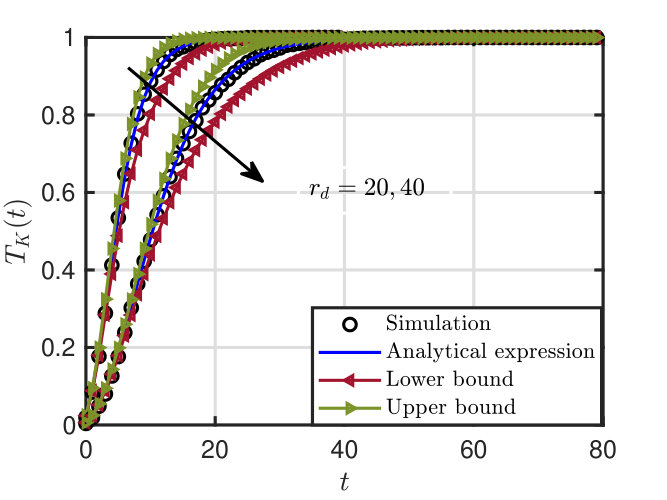 Figure 1
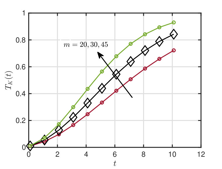 Figure 2
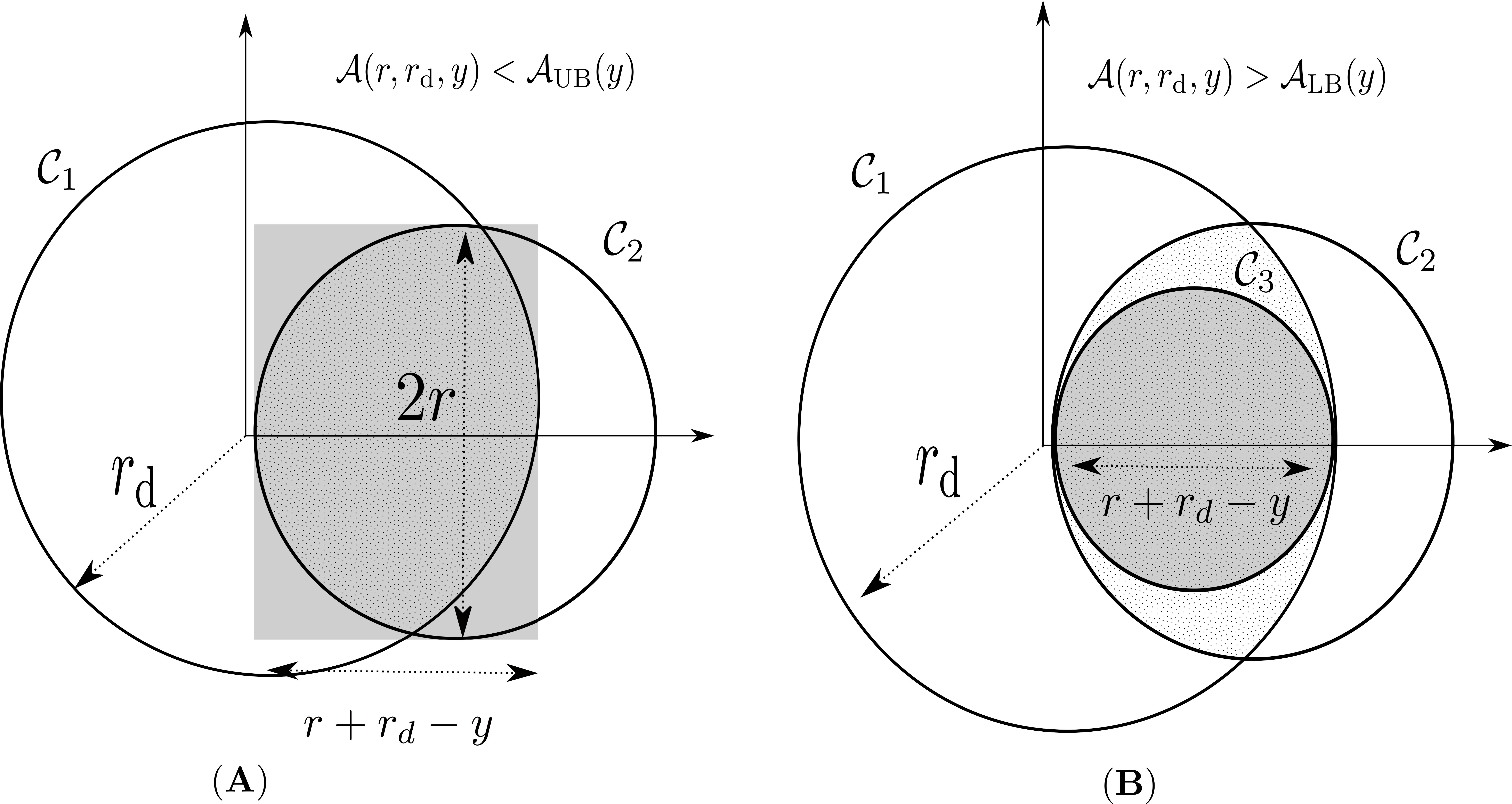 Figure 3
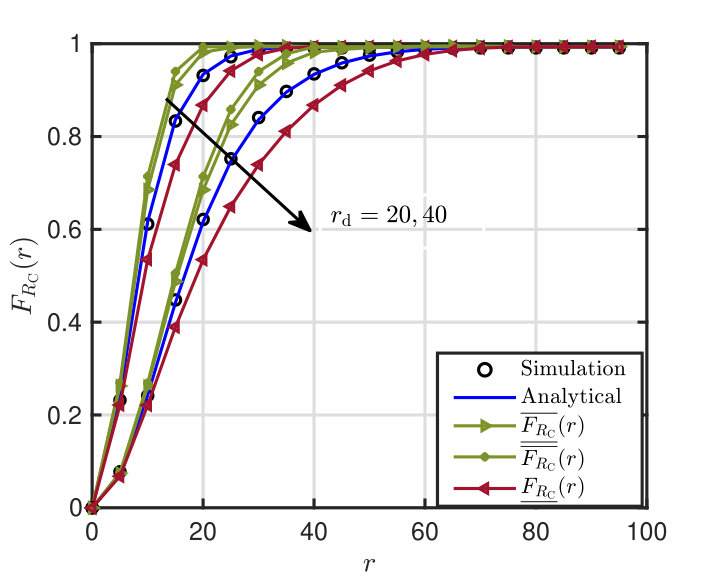 Figure 4
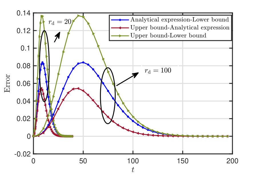 Figure 5
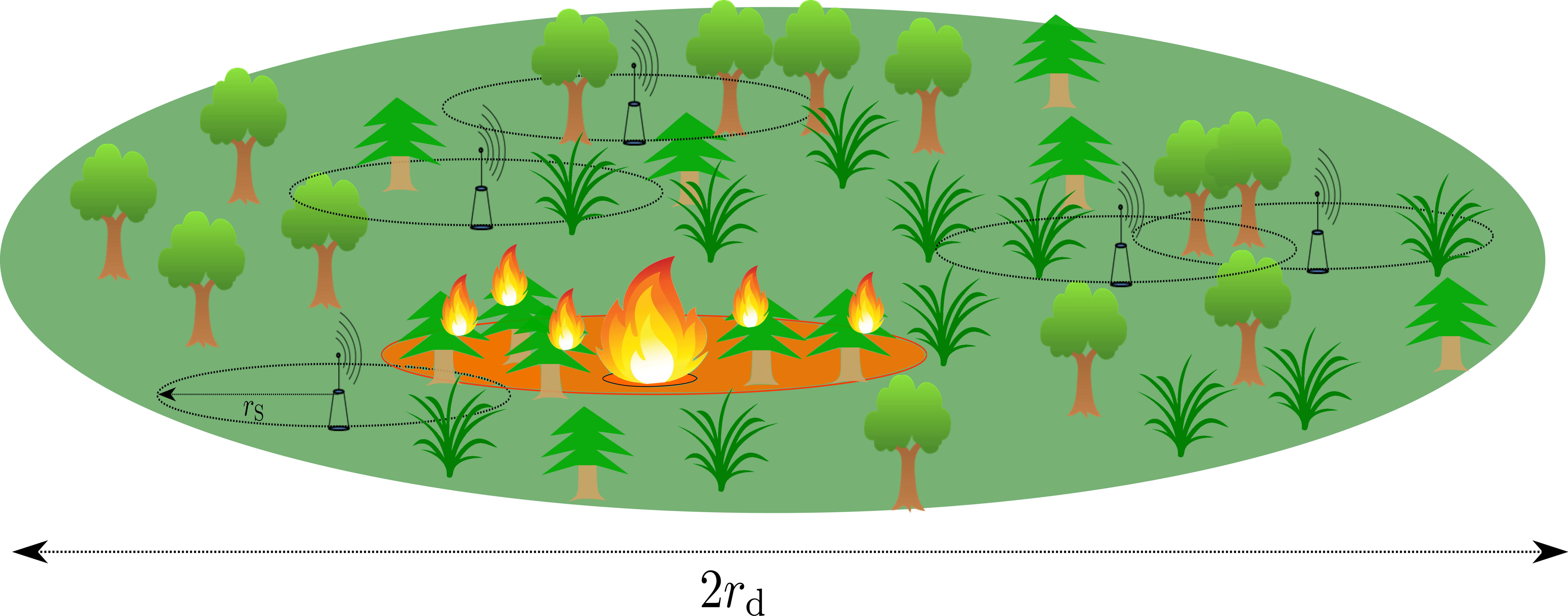 Figure 6
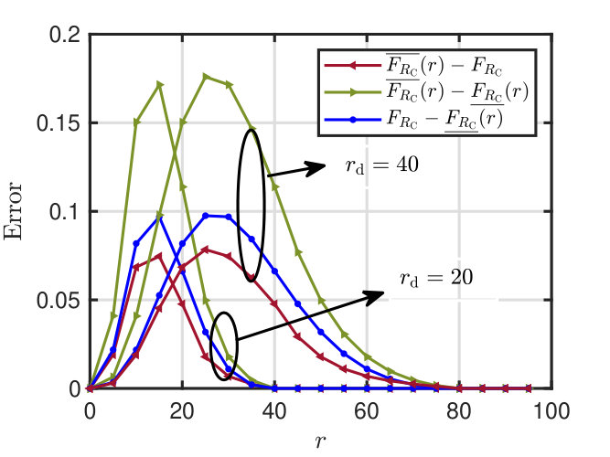 Figure 7
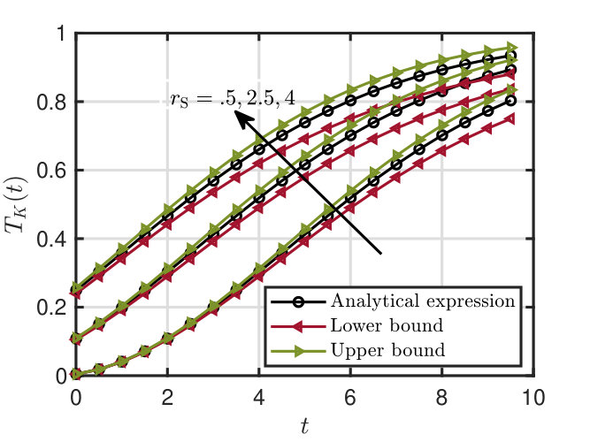 Figure 8
| Symbol | Definition |
|---|---|
| Ball of radius centred at . | |
| 2D FHPPP modeling location of sensors in the forest i.e. | |
| Density of wireless sensor network (number of sensors per unit area). | |
| The fixed sensing radius of each sensor. | |
| The location of the th sensor. | |
| Sensing region of sensor i.e. | |
| Total sensing area of all sensors. | |
| Area of intersection between two circles located distance apart with radii and . | |
| Minkowski addition operator. | |
| L-2 norm of . | |
| Random variable denoting the total number of points of located inside the set . | |
| Intersection between the circles and . | |
| Area of any set . |
Peer Reviews
No public reviews on file for this paper yet. If you reviewed it on a platform where reviews are public (OpenReview, ICLR, NeurIPS, ICML), you can paste yours below so the community can read it here.
Videos
No videos yet. Explain this paper in a talk, walkthrough, or lecture? Add one.
On Detection of Critical Events in a Finite Forest using Randomly Deployed Wireless Sensors
Kaushlendra K. Pandey, Abhishek K. Gupta
Department of Electrical Engineering
Indian Institute of Technology Kanpur, India
Email: [email protected], [email protected]
Abstract
Ecosystem of a forest suffers from many adverse events such as wild-fire which can occur randomly anywhere in the forest and grows in size with time. This paper aims to analyze performance of a network of randomly deployed wireless sensors for the early detection of these time-critical and time-evolving events in a forest. We consider that the forest lies in a confined space (e.g. a circular region) and the wireless sensors, with fixed sensing range, are deployed within the boundary of forest itself. The sensing area of the network is modeled as a finite Boolean-Poisson model. In this model, the locations of sensors are modeled as a finite homogeneous Poisson Point Process (PPP) and the sensing area of each sensor is assumed to be a finite set. This paper aims to answer questions about the proximity of a typical sensor from a randomly occurred event and the total sensing area covered by sensors. We first derive the distribution of contact distance of a FHPPP and the expression of the capacity functional of a finite Boolean-Poisson model. Using these, we then derive the probability of sensing the event at time , termed event-sensing probability.
I Introduction
The ecosystem and biodiversity of forests suffer from various natural and artificial events including wild-fires and spread of disease [1, 2]. The past literature has suggested that such events can be controlled to avoid severe loss by designing a mechanism for early detection of these events. One way to build an efficient alarm system for early detection of these time-critical events is by using wireless sensor network (WSN) of fire sensors deployed in forest. Wireless sensor networks refers to network of sensors connected via wireless links. WSNs are regarded as a cost-effective and inexpensive solution to jointly detect an event/events including fire over an area. However, while deploying a sensor network, it is important to understand the impact of the sensor density on the proximity of these critical events and the sensing region covered by these sensors in order to ensure that events are detected well in time.
The coverage performance of a WSN with sensors having fixed disk sensing range is analyzed in [3]. Readers are advised to refer to [4] for an extensive literature survey discussing the coverage and connectivity analysis of WSNs. The performance of a WSN can be characterized via various metrics, e.g. the distance of the closest sensor from an event (termed contact distance) or the probability that the event is sensed by at least one node of the WSN (termed event sensing probability). The deterministic deployment of sensor nodes may not be possible in the forests where terrains are not uniform. In these scenarios, sensors are generally deployed randomly. Tools from stochastic geometry provide a tractable framework to study the coverage of random networks including WSN [5]. The coverage performance of infinite random WSNs was well studied in the past literature [6]. Modeling of wireless sensor nodes as point process can be justified owing to their random deployment and connectivity mechanism [7]. Poisson point process (PPP) is one example of point process which has been widely used in the past literature owing to their tractability. For example, coverage analysis of wireless sensor network modeled as PPP is performed in [8]. In [9], PPP is used to model a sensor network with sensors acting as data collectors and transmitters to evaluate performance of this network. The coverage analysis of WSN with deterministic sensing range of individual sensors was performed in [10] by modeling this network using Boolean-Poisson model [11]. Although sensors are moving with time, authors have only considered a particular time snapshot where sensors locations form a PPP. Other point processes such as binomial point process (BPP), finite PPP are also used in the past literature. For example, WSN has been modeled as BPP. In [12], the authors presented a closed-form analytical expression for the moment generating function of the interference at the origin. In [13], authors presented the closed form expression for the different distance distribution of BPP. In [14], authors studied the distance distribution in a multi-hop network with nodes uniformly distributed in a square.
The expression for CDF of contact and nearest neighbor distance for homogeneous infinite PPP is available in [5]. The expression for capacity functional for a homogeneous PPP is derived in [11]. Since the forest lies in finite space, the deployed sensor network is also finite. There has been past research to investigate distribution of various distances among nodes that are uniformly distributed in a confined space. In [15], the authors derived the cumulative distribution function (CDF) of the distance between two randomly located mobile devices. In [16], authors have considered wireless nodes to be uniformly located within a square and calculated the distribution of the distance of the -th neighbor along with the distance between two randomly selected nodes. The performance of a sensor network modeled as a Boolean process with nodes located as PPP in a confined space to detect a dynamic and time-evolving event, for example, its coverage probability and the closest distance of the nearest sensor of this network from an arbitrary point in the same space was not studied in the past work which is the main focus of this paper.
In this paper, we consider a finite wireless sensor network with sensors in a confined circular forest. Each sensor node has an associated sensing range. The completed sensing range of the network is modeled as a finite Boolean-Poisson model. In this model, the locations of sensors (termed germs) are modeled as a finite homogeneous PPP (FHPPP) and the sensing area of each sensor (termed grain) is assumed to be a finite set. We first assume that the target critical event to be sensed/detected can occur uniformly anywhere in the forest. We then compute the distribution of distance of the nearest sensor from the occurrence point of this event. We also derive the expression for the capacity functional of finite Boolean model which help us derive the probability that the event is sensed by at least one sensor at time .
II System model
This paper presents the coverage-analysis of time-critical and dynamic events (e.g. wild-fires) occurred anywhere in the forest with the help of wireless sensors deployed randomly in the forest. The list of important symbols and notation is represented in table I.
We assume that the forest is modeled as a 2D ball with center at the origin and radius . The sensor nodes have a fixed sensing radius around them and are deployed to sense any time-critical event which can occur randomly and uniformly in the forest. We model the coverage area of the sensor network as a Boolean-Poisson model . In this process, the locations of sensor are modeled as a FHPPP with intensity
[TABLE]
where is the mean number of sensors deployed in the forest. Here, denotes the location of sensor. Let denote the density of this PPP inside the ball . Although this paper considers the forest to be confined in a circular region but the result obtained in the paper can be extended to analyze performance in forests of any arbitrary shape. Since, we have assumed that each sensor have a fixed sensing range , the occupied space by the sensor network is given by:
[TABLE]
Modelling events and their time-evolution: Let the occurrence/starting/center point of a target event be denoted by . The location of is assumed to be uniformly distributed in the forest . In other words, the probability density function of the distance of from the origin is given by
[TABLE]
As stated earlier, we consider events that are time-evolving (in particular growing with time). At time , the event’s envelop is denoted by set that contains the event occurrence point . The envelop size and shape at time will depend on the event type and its propagation/evolution characteristics. Consider an example of wild-fires in the absence of wind. Once a fire has occurred at the location , fire will increase in all directions with constant speed . Hence, at time , the fire envelop will be a circle, expressed as .
III Distance Distributions
In this section, we will derive the CDFs of contact distance of the event and the nearest neighboring sensor distance of a typical point for the FHPP .
III-A CDF of the contact distance of the event
The contact distance of the event is a random variable denoting the distance of closest sensor from the event occurrence point . It has been assumed that is independent of . In other words, is the distance of the nearest point of a finite homogeneous PPP from a reference location uniformly located inside the range of the finite PPP.
Let us first condition on the location of . The conditional CDF of the event contact distance at is the probability that nearest sensor from the location is at distance less than or equal to . Mathematically,
[TABLE]
Let the notation denote the total number of points of falling in ball . Therefore, denotes the void probability i.e. the probability that no point of falls in the ball . Therefore
[TABLE]
Theorem 1**.**
The CDF of the contact distance of an event for a FHPPP with density is given as
[TABLE]
Proof:
See Appendix A. ∎
Remark 1**.**
The case in Theorem 1 refers to the case where there is no sensor in the forest, and hence the distance to the nearest sensor is taken as . This is an artifact of PPP that there is zero point of PPP in a finite range with certain probability.
III-B CDF of the nearest neighbor sensor distance from a typical sensor
The nearest neighbor sensor distance is defined as the distance of a typical sensor to its nearest neighbor sensor. In the case of finite homogeneous PPP, the CDF of contact distance and nearest neighbor distance will be the same (See Appendix B for the proof). Therefore,
[TABLE]
Similar to the previous case, refers to the scenario where there is no other sensor in the forest.
Theorem 2**.**
The expressions for the upper bound , and the lower bound , on the CDF of the event contact distance is given by:
[TABLE]
where,
[TABLE]
[TABLE]
Proof:
See Appendix C. ∎
Remark 2**.**
Another (loose) upper bound on the CDF of the event contact distance is given as:
[TABLE]
Proof: The upper bound can be achieved by replacing the intersecting area with its corresponding upper bound .
III-C Asymptotic behavior of with while keeping fixed:
III-C1 As
In this case, the term , therefore, the contact distance distribution will be:
[TABLE]
III-C2 As
In this case, the term . Hence, the contact distance distribution will be:
[TABLE]
When , FHPPP trivially converges to a homogeneous PPP with intensity .
IV Capacity functional of FHPPP and the event sensing probability
Let the set denote the envelop of an event that have occurred centered at location . Recall the assumption that is uniformly located in and independent of FHPPP. We assume that the event envelop is expanding with time .
The event sensing probability at time is the probability that the event envelop is sensed by at least one sensor of the WSN. Note that the event will be sensed if and only if the intersection of with is non empty. Hence,
[TABLE]
Similar to the previous section, we will start the derivation with conditioning on the location . Conditioned on , at time , is the probability that an event started at center is sensed at time . Mathematically, it can be written as:
[TABLE]
Note that this is the capacity functional of finite Boolean-Poisson model evaluated at the set .
Theorem 3**.**
The event sensing probability at time is given as
[TABLE]
Here, denotes the conditional event sensing probability at time , conditioned on the starting location of the event and is given as
[TABLE]
where is the complement set of and is and denotes the Minkowski sum. Minkowski sum of any two set is defined as .
Proof:
See Appendix D. ∎
Remark 3**.**
It can be easily seen that if is a 2-dimensional ball then complement of will be itself. Therefore, will be .
Remark 4**.**
For the case of wild-fire, the denotes fire-envelop which may take some shape depending upon the presence or absence of wind and its direction. In the absence of wind, the fire envelop expands with a velocity of in all directions. At time , the fire envelop will be a point located at the point and at time it will become a circle with radius .
Now, is the Minkowski sum of two balls which is equal to a ball of aggregate radius
[TABLE]
*The fire sensing probability of a fire started at a typical point at time is given as: *
[TABLE]
Corollary 1**.**
The coverage probability of a random point can be trivially achieved by putting and is given as
[TABLE]
Theorem 4**.**
Bounds on the event sensing probability is given by:
[TABLE]
where , and .
Another bound over the event sensing probability is given by:
[TABLE]
IV-A Asymptotic analysis
IV-A1 As
In this case, the term . Hence,
[TABLE]
IV-A2 As
In this case, the term which is not a function of . Let us denote this term as . Hence,
[TABLE]
Therefore, the expression of the event sensing probability reduces to the capacity functional of Boolean-Poisson model as given in [11].
V Simulation results and analysis
In this section, we present some numerical results to validate our analysis and provide insights about the system.
V-1 CDF of contact distance and bounds
Fig. 2 shows the CDF of the nearest neighbor distance and corresponding upper and lower bounds for two values of . It can be been easily seen that increasing , will reduce the CDF because points will spread to far locations. Fig. 3 depicts the deviation of bounds from the exact values.
V-2 Event sensing probability and corresponding bounds
We now consider the case of wild-fires. Recall our assumption that fire envelop takes a circular shape with radius . Fig. 4 shows the variation of fire sensing probability and the deviation of bounds from exact values at time . Intuitively, the fire sensing probability will increase with time. It is observed from Fig. 5 that the maximum error does not change much with respect to . Therefore, the bounds may be tight even for higher values of .
V-3 Impact of sensing range and number of sensors
Fig. 6 shows the impact of increasing sensing range on the fire sensing probability at time for a WSN with 40 sensors deployed in a forest with radius 40 units. We can observe that increasing the sensing range of sensors will increase the fire sensing probability. Hence, the critical time required to sense a fire with certain probability can be increased by increasing the sensing range which helps in early detection of fire. Fig. 7 shows the trade-off between the mean number of sensors () and the sensing range () for the fire sensing probability, while keeping fixed. Note that denotes the sum of sensing areas of all sensors, and thus was used for the fair comparison. It can be observed that increasing the density of sensors have a higher impact on the fire sensing probability than increasing the individual sensor’s sensing range. This can be justified in the following way. Increasing the number of sensors while reducing individual sensor’s sensing range spreads the sensing region across the forest. On the other hand, increasing the individual sensor’s sensing range while reducing the number of sensors localizes the sensing region .
VI Conclusion
This paper studies the dynamic event sensing performance of a randomly deployed wireless sensor network in a finite area (e.g. forest) modeled by a FHPPP. The paper analyzes the proximity of the wireless sensor network to an event, whose location is uniformly distributed across the entire forest. In particular, we study the event sensing probability after time since the occurrence of the event. This paper presents an analytical expression for the CDF of contact distance and nearest neighbor distance distribution of FHPPP. The bounds presented are tight and can be used for the asymptotic analysis of the distance distribution and capacity functional. Finally, the simulation results validate the theoretical analysis. There are numerous possible extensions of this work. We have considered a circular fire propagation model which is an ideal case; there are several other fire propagation model exits in the literature. These fire propagation models are more realistic and can provide better insights into the sensor density. In some seasons the forest is prone to fire therefore the seasonal variations can also be included in the analysis to optimize the number of active sensors and to minimize the energy consumption of the sensor network.
Appendix A Proof of Theorem 1
The void probability of FHPPP for the set is given as
[TABLE]
Here, is due to the PGFL (probability generating functional) of finite PPP [5]. After de-conditioning over , we get (2).
Appendix B Proof of (3)
The distribution of the distance from the nearest neighbor sensor from any point is given as
[TABLE]
Here, is due to Campbell Mecke’s theorem. is the reduced palm distribution and it is equal to the for a PPP due to Slivnyak’s theorem (step (b)).
Appendix C Proof of Theorem 2
In order to find the upper and lower bound of the contact distance , consider the following integral:
[TABLE]
For range , the intersecting area is equal to and the contribution of this range to the above integral is .
For range , the intersecting area
[TABLE]
The integral for the range can not further simplified to its closed form. Hence, we will try to replace with its upper and lower bound.
C-1 Proof of upper bound
Fig. 8(A) shows the intersecting region by the dotted area. The area of the rectangular shaded serves as an upper bound for the area of the intersecting region. This rectangle has width and height .
C-2 Proof of lower bound
Let the two circle be and , of radius and respectively. Without loss of generality, assume . Let the center of is located at the origin. Let have its center at . Therefore the distance between center of the two circle is . We have drawn a circle , of radius centered at . It is clear from Fig.8(B) that circle will touch and only at one point and the distance between the two is the diameter of . Therefore, is completely under the intersecting region. Hence, its area serves as the lower bound for the intersecting area.
Appendix D Proof of Theorem 3
Conditioned on the occurrence point , the event sensing probability is given as
[TABLE]
Here, is obtained from the PFGL of FHPPP, and is due to the fact that integrating the product of indicators of two sets over results in the area of the intersection of these two sets.
The reference list from the paper itself. Each links out to its DOI / PubMed record.
- 1[1] K. Pandey and A. K. Gupta, “Modeling and analysis of wildfire detection using wireless sensor network with poisson deployment,” in Proc. IEEE ANTS , Dec. 2018.
- 2[2] D. M. Molina-Terrén, G. Xanthopoulos, M. Diakakis, L. Ribeiro, D. Caballero, G. M. Delogu, D. X. Viegas, C. A. Silva, and A. Cardil, “Analysis of forest fire fatalities in southern europe: Spain, portugal, greece and sardinia (italy),” International Journal of Wildland Fire , vol. 28, no. 2, pp. 85–98, 2019.
- 3[3] G. S. Kasbekar, Y. Bejerano, and S. Sarkar, “Lifetime and coverage guarantees through distributed coordinate-free sensor activation,” IEEE/ACM Trans. on Netw. , vol. 19, no. 2, pp. 470–483, April 2011.
- 4[4] D. Simplot-Ryl, I. Stojmenovic, and J. Wu, “Energy efficient backbone construction, broadcasting, and area coverage in sensor networks,” Handbook of Sensor Networks , pp. 343–380, 2005.
- 5[5] J. G. Andrews, A. K. Gupta, and H. S. Dhillon, “A primer on cellular network analysis using stochastic geometry,” ar Xiv preprint ar Xiv:1604.03183 , 2016.
- 6[6] F. Baccelli and B. Błaszczyszyn, Stochastic Geometry and Wireless Networks , 2nd ed. NOW Publishers, 2009, vol. 1.
- 7[7] M. Haenggi, Stochastic geometry for wireless networks . Cambridge University Press, 2012.
- 8[8] P.-J. Wan and C.-W. Yi, “Coverage by randomly deployed wireless sensor networks,” IEEE/ACM Transactions on Networking (To N) , vol. 14, no. SI, pp. 2658–2669, 2006.