A mechanism for balancing accuracy and scope in cross-machine black-box GPU performance modeling
James D. Stevens, Andreas Kl\"ockner

TL;DR
This paper introduces a flexible, black-box approach for creating customizable performance models of GPU kernels that balance accuracy, speed, and generalizability across multiple architectures.
Contribution
It presents a novel method for automatic kernel operation counting, model formulation, and calibration, enabling tailored GPU performance modeling without manual hardware statistics collection.
Findings
Models accurately predict execution times across multiple GPU architectures.
The approach effectively balances model complexity with evaluation speed.
Demonstrated on matrix multiplication, DG differentiation, and finite difference kernels.
Abstract
The ability to model, analyze, and predict execution time of computations is an important building block supporting numerous efforts, such as load balancing, performance optimization, and automated performance tuning for high performance, parallel applications. In today's increasingly heterogeneous computing environment, this task must be accomplished efficiently across multiple architectures, including massively parallel coprocessors like GPUs. To address this challenge, we present an approach for constructing customizable, cross-machine performance models for GPU kernels, including a mechanism to automatically and symbolically gather performance-relevant kernel operation counts, a tool for formulating mathematical models using these counts, and a customizable parameterized collection of benchmark kernels used to calibrate models to GPUs in a black-box fashion. Our approach empowers a…
Click any figure to enlarge with its caption.
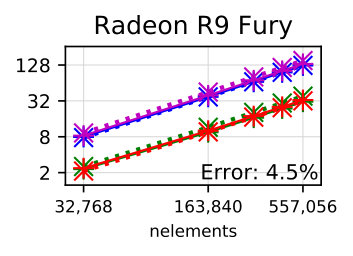 Figure 1
 Figure 2
 Figure 3
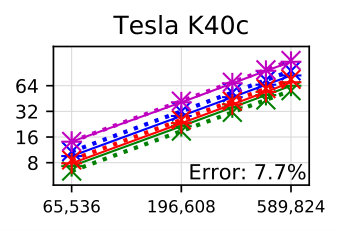 Figure 4
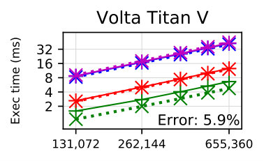 Figure 5
 Figure 6
 Figure 7
 Figure 8
 Figure 9
 Figure 10
 Figure 11
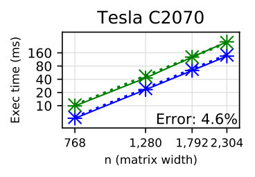 Figure 12
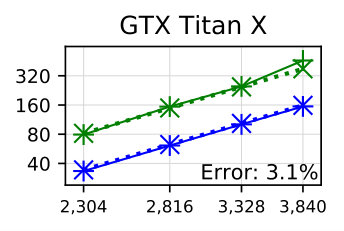 Figure 13
 Figure 14
 Figure 15
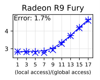 Figure 16
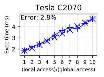 Figure 17
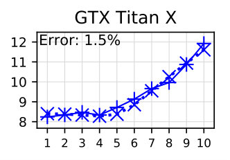 Figure 18
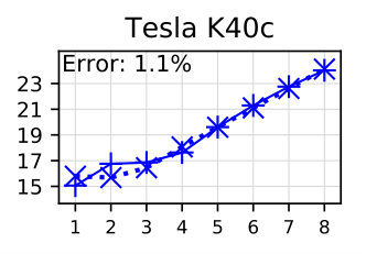 Figure 19
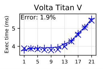 Figure 20
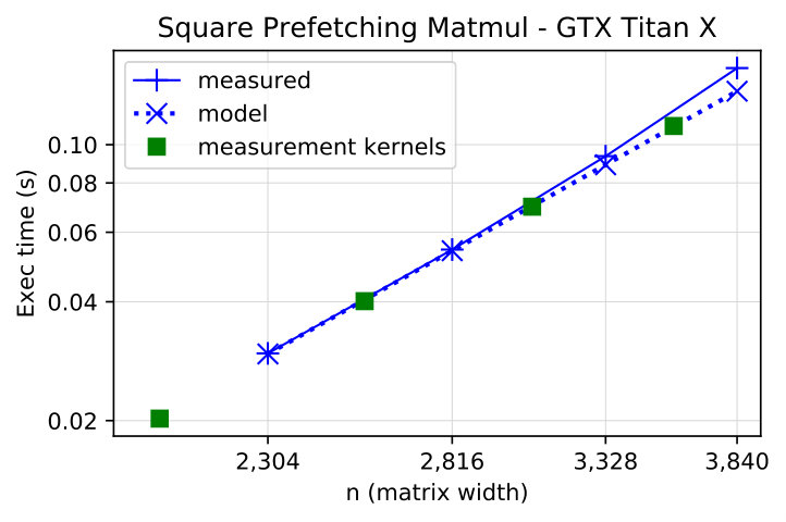 Figure 21
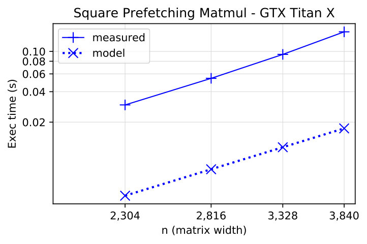 Figure 22
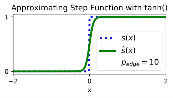 Figure 23
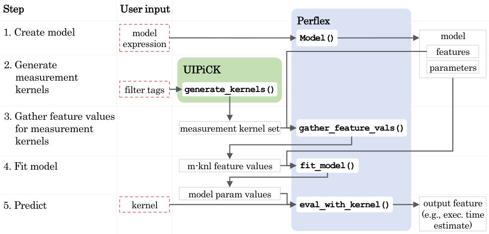 Figure 24
| Local | Loop | |||
|---|---|---|---|---|
| Array | Ratio | strides | Global strides | stride |
| a | n/16 | {0:1, 1:n} | {0: 0, 1:n*16} | 16 |
| b | n/16 | {0:1, 1:n} | {0:16, 1:0} | 16*n |
| GPU (Generation) | OpenCL/Platform/Driver Info |
|---|---|
| Nvidia Titan V (Volta) | OCL 1.2, CUDA 10.0.246 (410.93) |
| Nvidia GTX Titan X (Maxwell) | OCL 1.2, CUDA 10.0.292 (410.104) |
| Nvidia Tesla K40c (Kepler) | OCL 1.2, CUDA 9.1.84 (390.87) |
| Nvidia Tesla C2070 (Fermi) | OCL 1.2 CUDA 9.1.84 (390.116) |
| AMD Radeon R9 Fury (GCN 3) | OpenCL/ROCm 1.2.0-2019020110 |
| ROCm platform HSA runtime 1.1.9-49-g39f1af5 | |
| Kernel 4.19 |
| Param. | |||
|---|---|---|---|
| Feature | val. (s) | MCG | Rate |
| f32 add | SG | op/s | |
| f32 mul | SG | op/s | |
| f32 madd | SG | op/s | |
| SG | B/s | ||
| WI | B/s | ||
| WI | B/s | ||
| WI | B/s | ||
| WI | B/s | ||
| SG | B/s | ||
| local barrier | WG |
Peak
FLOP/s B/s |
|
| launch group | WG | ||
| launch kernel | K | ||
| () | N/A |
Peer Reviews
No public reviews on file for this paper yet. If you reviewed it on a platform where reviews are public (OpenReview, ICLR, NeurIPS, ICML), you can paste yours below so the community can read it here.
Videos
No videos yet. Explain this paper in a talk, walkthrough, or lecture? Add one.
\corrauth
James D. Stevens; 201 N Goodwin Ave; Urbana, IL 61801
A mechanism for balancing accuracy and scope in cross-machine
black-box GPU performance modeling
James D. Stevens11affiliationmark:
Andreas Klöckner11affiliationmark:
11affiliationmark: University of Illinois at Urbana-Champaign; Deptartment of Computer Science
Abstract
The ability to model, analyze, and predict execution time of computations is an important building block that supports numerous efforts, such as load balancing, benchmarking, job scheduling, developer-guided performance optimization, and the automation of performance tuning for high performance, parallel applications. In today’s increasingly heterogeneous computing environment, this task must be accomplished efficiently across multiple architectures, including massively parallel coprocessors like GPUs, which are increasingly prevalent in the world’s fastest supercomputers. To address this challenge, we present an approach for constructing customizable, cross-machine performance models for GPU kernels, including a mechanism to automatically and symbolically gather performance-relevant kernel operation counts, a tool for formulating mathematical models using these counts, and a customizable parameterized collection of benchmark kernels used to calibrate models to GPUs in a black-box fashion. With this approach, we empower the user to manage trade-offs between model accuracy, evaluation speed, and generalizability. A user can define their own model and customize the calibration process, making it as simple or complex as desired, and as application-targeted or general as desired. As application examples of our approach, we demonstrate both linear and nonlinear models; these examples are designed to predict execution times for multiple variants of a particular computation: two matrix-matrix multiplication variants, four Discontinuous Galerkin (DG) differentiation operation variants, and two 2-D five-point finite difference stencil variants. For each variant, we present accuracy results on GPUs from multiple vendors and hardware generations. We view this highly user-customizable approach as a response to a central question arising in GPU performance modeling: how can we model GPU performance in a cost-explanatory fashion while maintaining accuracy, evaluation speed, portability, and ease of use, an attribute we believe precludes approaches requiring manual collection of kernel or hardware statistics.
keywords:
Performance model, GPU, Microbenchmark, Code generation, Black box, OpenCL
1 Introduction
Maximizing computational performance requires tailoring an application implementation to the target architecture. As a result, obtaining and maintaining good performance in a heterogeneous computing environment necessitates the ability to efficiently decide between multiple mathematically equivalent program variants. Being able to model, interpret, and predict the execution time of computational kernels can provide insight into factors contributing to computation cost, and doing so in an automated, architecture-independent fashion is a key step toward the automation of performance tuning for complicated, modern, vector-based, massively parallel processor architectures including recent CPUs and GPUs.
GPUs, originally designed for rapid graphics rendering, have highly parallel single instruction, multiple thread (SIMT) architectures that make them particularly useful for data-parallel problems. Over the last decade, general purpose GPU programming has risen in popularity. GPUs are increasingly prevalent in the world’s fastest supercomputers, and are being utilized in an expanding body of applications including machine learning and artificial intelligence. GPU programming has been facilitated by the release of general purpose GPU programming systems, including Nvidia CUDA in 2007 and the Open Computing Language (OpenCL) in 2009 (Nickolls et al., 2008; Munshi et al., 2011).
Tailoring a performance model to a particular computation on a single hardware device may yield high accuracy. When broadening the scope of architectures and computations targeted by a model, achieving high accuracy becomes increasingly difficult. We present a mechanism for putting the user in control of this trade-off between model accuracy and generalizability with an approach for creating custom performance models that is realized on top of, though technically not dependent on, a program transformation system.
We consider this contribution a building block to provide guidance in exploring the vast search space of possible and, from the point of view of the result, equivalent program variants, by either a developer or an auto-tuning compiler. We view the models constructed within our framework as more economical alternatives to evaluating execution time of computational kernels than, for example, using actual on-device timing runs. Our system primarily targets execution on modern GPU hardware, as exposed in, for example, the CUDA or OpenCL compute abstractions. To facilitate portability and maximize ease of use, the system makes few assumptions about the internal organization of the hardware, and device-specific parameters are obtained from a black-box model-calibration process that needs to run precisely once per model per hardware device used. We demonstrate that this cross-machine, black-box, microbenchmarking approach to analytical performance modeling can predict kernel execution time well enough to determine which of multiple implementation variants will yield the shortest execution times.
We review related performance modeling work in Section 9, and discuss two recent surveys of the current GPU performance modeling landscape, Madougou et al. (2016) and Lopez-Novoa et al. (2015). Like the survey authors, we find that many existing GPU performance models predict well for a particular application or architecture but are not easily portable across machines. Most require knowledge of hardware or application characteristics, often gathered manually, and significant effort to construct and use. Compared to analytical approaches, learning and statistical techniques tend to be more hardware-flexible, but the models produced are less accessible to users from the standpoints of both design and interpretability; assumptions and limitations about model predictive power, fidelity, and range of applicable programs and hardware tend to be less clear. Madougou et al. (2016) conclude that software utilizing these methods may be difficult to use for users without good knowledge of statistical methods. None of the approaches we surveyed provide users any significant control over the model expression or (micro)benchmark design.
The following combination of factors distinguishes our work from previous GPU performance modeling work, and comprises our primary contributions:
- •
Our approach allows broad customization of the mathematical model not available in previous work. A user can rely on predefined generic models or define their own model, making it as simple or as complex as desired, as application-targeted or as general-purpose as desired.
- •
Similarly, our approach allows for complete customization of the set of measurement computations used to compute the model parameters during the model calibration process.
- •
We automate the gathering of all performance-relevant kernel features used to model execution time. These features are gathered before compilation by examining our polyhedrally-based program representation.
- •
In the example models we show in Section 8, the only hardware statistic required is the sub-group size, which is 32 on all current Nvidia and AMD hardware generations. This demonstrates that a black-box approach to performance modeling can capture execution cost behavior with very limited explicit representation of hardware characteristics. (Sub-groups and other details of the OpenCL machine model are discussed in Section 1.2.)
- •
Models created using our approach are hardware vendor- and generation-independent, and we demonstrate performance on an AMD GPU and four generations of Nvidia GPUs.
- •
Models created using our approach are amenable to human understanding: through the exposed parameters and their known meanings, it becomes possible to reason about which parts of kernel execution cost are attributed to which specific operations.
- •
By making use of a polyhedrally-based program representation, we obtain precise counts of various units of work performed by the static-control part of a program. The counts obtained are parametric in the problem size, allowing us to amortize counting work over repeated applications of the model to the same kernels with varying problem size.
- •
To help identify and measure cost contributions from individual memory accesses, we introduce a code transformation that can remove unrelated operations from a computation, thereby obtaining a kernel exercising the targeted memory access.
- •
To help model temporal overlap, e.g., between computation and memory operations, we introduce a modeling paradigm that reflects the reduced apparent cost of the overlapped fraction of computation. We demonstrate the use of the resulting, complex model expressions within our (unmodified) black-box measurement and timing facilities to provide accurate performance modeling even in the challenging case of overlapped operations.
1.1 Practical Realization of the Proposed Performance Modeling
Framework and the Loopy Program Transformation System
For the representation of programs, as well as to enable our static counting of operations, we rely on the Loopy program transformation system (Klöckner, 2014, 2015). While we make use of certain capabilities available in Loopy, this is not a hard dependency, in that any system offering a given interface could assume this role. In this section, we first briefly introduce Loopy and then describe that abstract interface.
Loopy is a programming system for array computations that targets CPUs, GPUs, and other, potentially heterogeneous, compute architectures. This system keeps the mathematical intent of a computation strictly separated from computational and performance-related minutiae. To attain that goal, Loopy realizes programs as objects in a host programming language (Python in this concrete case) that can be manipulated from their initial, “clean,” mathematical statement into highly device-specific, optimized versions via a broad array of transformations. From these program objects, Loopy generates and executes source code in a range of output languages, including OpenCL, the output language we use for Loopy programs demonstrated in this work.
Our methodology to automatically gather the kernel statistics underlying kernel features that are used by our modeling process leverages the Loopy programming system in a number of ways:
- •
we express our kernels in its intermediate representation based on a generic OpenCL/CUDA-style machine model,
- •
we use its program transformation vocabulary to obtain computationally different but mathematically equivalent variants of our measurement kernels,
- •
we use it to generate OpenCL C-level source code for the various target machines on which we evaluate our model. While Loopy is able to target a much larger range of output languages (e.g., C, OpenMP [Open Multi-Processing] + SIMD [single instruction, multiple data], OpenCL, ISPC [Intel SPMD Program Compiler], CUDA), we limit ourselves to only OpenCL in keeping with our focus on GPUs, and finally,
- •
we make use of Loopy’s polyhedrally-based internal representation to support the automatic extraction of kernel statistics.
One of the primary design goals of Loopy, Perflex, and UIPiCK is to avoid the need to write detailed OpenCL- or CUDA-level code manually, thereby reducing development cost. We view this reduction of manual kernel construction as a valuable feature. Nonetheless, our modeling approach could be used with less reliance on Loopy, or none at all.
For example, the automated statistics-gathering piece of our work is notionally independent of our modeling process in the sense that, while it is convenient to have the ability to automatically extract the kernel features being used in our models, it is not technically necessary and could be achieved either by hand or in a technologically different manner. One tool that could facilitate the collection of statistics to compute feature values for a non-Loopy kernel is the Polyhedral Extraction Tool, a library for extracting a polyhedral representation from C source code (Verdoolaege and Grosser, 2012).
Additionally, the process of predicting performance via model evaluation can be easily separated from the model construction and calibration process. Once a model has been calibrated and parameter values obtained using Perflex and UIPiCK, if a developer has a different technique to obtain statistics and feature values for their application kernel, or if these values are known by design, they may use the parameter values to predict performance independently from Perflex and Loopy.
To accommodate legacy code in the existing system, we would also like to highlight the capability of Loopy to ingest a dialect of Fortran 77, as described in Klöckner (2015); Klöckner et al. (2016).
1.2 OpenCL Machine Model
Program representation in Loopy relies on the OpenCL machine model (Munshi et al., 2011) for semantics, and typical GPU hardware mappings thereof inspire the models we use to demonstrate our approach. A very brief overview of the OpenCL machine model will introduce terminology used throughout the following discussion.
The OpenCL model considers two levels of concurrency, each explicitly exposed to the abstraction by the programmer in the form of a multi-dimensional grid. Each integer point in the grid is called a work-item. A rectangularly-indexed set of work-items forms a work-group, and a rectangularly-indexed set of work-groups forms a grid (or NDRange), which is the unit in which work is expressed to the abstraction. Additionally, a sub-group is an implementation-dependent grouping of work-items within a work-group which we assume to approximate the effective vector width with which the architecture issues instructions. Aside from barrier synchronization across the work-items in a work-group, individual work items are assumed to be independent. Item indices within a work-group are termed local indices or local IDs, and indices of a work-group in the grid are termed group indices or group IDs. We will use symbols like lid(0) to denote the local ID along axis 0 and gid(1) to denote the group ID along axis 1. We assume, in keeping with implementations available in the marketplace, that work-groups are implemented by first mapping contiguous work-items along the lowest-numbered axis to adjacent SIMD lanes, subsequently to simultaneous multithreading (SMT), and finally to sequential execution. Likewise we assume that work-groups are mapped to individual execution cores, potentially mapping multiple work-groups onto one core depending on capacity.
2 Illustrative Example
As an introduction to our modeling approach, consider the following simple, illustrative example use case. Suppose a user wants to model and predict the execution time of square matrix-matrix multiplication on a GPU. In this case, we will only predict execution times for a single program variant employing an algorithm which divides each matrix into tiles and avoids some repeated access to global memory by prefetching these tiles into local memory shared between threads before performing the multiplication and addition.
2.1 Kernel Creation and Transformation
To construct an initial program representation of the matrix-matrix multiplication workload using Loopy, we first specify the mathematical intent:
⬇ knl = lp.make_kernel("{[i,j,k]: 0<=i,j,k<n}",
"c[i,j] = sum(k, a[i,k]*b[k,j])")
Without any code transformations, Loopy produces a sequential algorithm looping over each index, as in the following OpenCL code:
⬇ float acc;
for (int j = 0; j <= -1 + n; ++j)
for (int i = 0; i <= -1 + n; ++i)
{
acc = 0.0f;

**for** (**int** k = 0; k <= -1 + n; ++k)

  acc = acc + a[n*i + k] * b[n*k + j];

c[n*i + j] = acc;
}
To expose levels of concurrency in the form of loops that will become parallelized, we perform loop-splitting transformations:
⬇ knl = lp.split_iname(knl, "i", 16)
knl = lp.split_iname(knl, "j", 16)
knl = lp.split_iname(knl, "k", 16)
knl = lp.assume(knl, "n >= 1 and n % 16 = 0")
Each split_iname transformation divides one loop into two nested loops with the inner loop iterating over the specified number of index values (16). Without knowledge about the value of n, Loopy would need to add several conditional statements to prevent out-of-bounds array access. We avoid these conditionals by adding the assume transformation, yielding the following OpenCL code:
⬇ float acc;
for (int j_out = 0; j_out <= ...
for (int j_in = 0; j_in <= 15; ++j_in)
**for** (**int** i_out = 0; i_out <= ...

  **for** (**int** i_in = 0; i_in <= 15; ++i_in)

  {

    acc = 0.0f;

    **for** (**int** k_out = 0; k_out <= ...

      **for** (**int** k_in = 0; k_in <= 15; ++k_in)

        acc = acc +

            a[n*(16*i_out + i_in) + 16*k_out + k_in]

            *

            b[n*(16*k_out + k_in) + 16*j_out + j_in];

    c[n*(16*i_out + i_in) + 16*j_out + j_in] = acc;

  }
To parallelize loops, we tag loop indices with OpenCL thread indices:
⬇ knl = lp.tag_inames(knl,
"i_out:g.1, i_in:l.1, j_out:g.0, j_in:l.0")
This tag_inames transformation parallelizes loop(s) across thread indices as specified, i.e., "i_in:l.1" parallelizes the i_in loop across the lid(1) thread index. After tagging loop indices, we obtain the following OpenCL code:
⬇ float acc;
acc = 0.0f;
for (int k_out = 0; k_out <= ...
for (int k_in = 0; k_in <= 15; ++k_in)
acc = acc +

    a[n*(16*gid(1) + lid(1)) + 16*k_out + k_in] *

    b[n*(16*k_out + k_in) + 16*gid(0) + lid(0)];
c[n*(16gid(1) + lid(1)) + 16gid(0) + lid(0)] = acc;
Finally, to help amortize data motion cost, we perform prefetching transformations:
⬇ knl = lp.add_prefetch(knl, "a", ["i_in","k_in"])
knl = lp.add_prefetch(knl, "b", ["k_in","j_in"])
The two prefetching transformations load data from the specified array into local memory outside of the specified loop, yielding the following OpenCL kernel:
⬇ float acc;
acc = 0.0f;
__local float a_fetch[16*16];
__local float b_fetch[16*16];
for (int k_out = 0; k_out <= ((-16 + n) / 16); ++k_out)
{
barrier(CLK_LOCAL_MEM_FENCE);
a_fetch[16*lid(1) + lid(0)] =
a[n*(16*gid(1) + lid(1)) + 16*k_out + lid(0)];
b_fetch[16*lid(1) + lid(0)] =
b[n*(16*k_out + lid(1)) + 16*gid(0) + lid(0)];
barrier(CLK_LOCAL_MEM_FENCE);
for (int k_in = 0; k_in <= 15; ++k_in)
acc = acc + a_fetch[16*lid(1) + k_in] *

    b_fetch[16*k_in + lid(0)];
}
c[n*(16gid(1) + lid(1)) + 16gid(0) + lid(0)] = acc;
2.2 Model Creation, Calibration, and Evaluation
For simplicity in this example, we only predict execution times for a single program variant, so a very simple mathematical model may suffice. We model the execution time as
[TABLE]
where is matrix width, or, more generally a parameter which statically determines the size of the loop domain that is assumed to be known at runtime; is the number of multiply-add (“madd”) sequences executed by the algorithm; is a hardware-dependent parameter representing the effective cost (seconds) per madd for this program variant; and is execution time. We distinguish madd sequences from isolated multiplication or addition operations since many GPUs provide a specialized fused multiply-add (FMA) operator. We refer to quantitative kernel characteristics used in our models as kernel features. Input features, e.g., , appear in the model function, and output features, e.g., , are produced when evaluating a model function.
Our methods for automatically producing symbolic counts like in the form of piecewise quasi-polynomials will be discussed in Section 5. Now we need a value for parameter .
To determine this parameter value while treating the GPU as a black-box, we run measurement computations designed to reveal the appropriate cost. In this simple example we need the effective madd cost only for this particular program variant, so we determine this cost by running the same matrix multiplication variant on various sizes of matrices, computing and for each, and then calibrating our model by fitting the model function to the feature data to compute . More complex models that employ a microbenchmark approach to determine parameter values will be discussed in Section 8.
The following code fragments demonstrate how this is accomplished using our framework.
- Define the model shown in (1) by specifying wall time on the Nvidia GTX Titan X GPU as the output feature (f_cl_wall_time_nvidia_geforce), and providing the model expression. p_f32madd represents parameter and f_op_float32_madd specifies input feature :
⬇ model = Model("f_cl_wall_time_nvidia_geforce",
"p_f32madd * f_op_float32_madd")
2. Generate measurement kernels for model calibration using our parameterized collection of kernel generators, UIPiCK, which we describe in Section 7.1. To govern which generators are used and which kernel variants are produced by each generator, we pass filtering tags to the kernel collection identifying the desired computation and describing, for example, the data type of the arrays, the work-group dimensions, whether to prefetch data into local memory, or whether to assume that work-group dimensions divide evenly into the corresponding array dimensions. In this example, we generate square matrix multiplication kernel variants:
⬇ filter_tags = [
"matmul_sq", "dtype:float32", "prefetch:True",

"lsize_0:16", "lsize_1:16", "groups_fit:True",

"n:2048,2560,3072,3584"]
m_knls = KernelCollection(uipick.ALL_GENERATORS).generate_kernels(filter_tags)
Generator filter tags, consisting of a single value, e.g., matmul_sq, determine which generators run. This kernel collection includes all UIPiCK generators, but the matmul_sq tag filters out generators not executing a square matmul. In this case, only generators with a tag matching the user-supplied generator tag, matmul_sq, will execute, which leaves us with a single generator. Variant filter tags consist of argument:value pairs, e.g., dtype:float32, and determine which kernel implementation variants are produced by the generators. Each generator maintains a set of allowable values for each argument and generates one kernel for each set of arguments in the Cartesian product of allowable argument value sets. By passing a variant filter tag with argument values, the user can reduce the set of allowable values for that argument. In this example, we provide a set of four values for the problem size n and a single value for each of the remaining arguments, so four measurement kernels will be generated. We discuss kernel set generation and filtering further in Section 7.1.
- Compute input and output feature values for all measurement kernels:
⬇ m_knl_feature_values = gather_feature_values(
model.all_features(), m_knls)
Here we compute the two feature values found in our model, madd count and execution time, for each of the four measurement kernels. This uses our automatic kernel statistics gathering techniques described in Section 5.
- Fit model to feature value data, producing parameter values:
⬇ model_param_values = fit_model(
model, m_knl_feature_values)
We describe this calibration process in Section 7.2.
- Evaluate the model to predict execution time for a kernel:
⬇ exec_time = model.eval_with_kernel(
model_param_values, test_knl, {"n": 1024})
Figure 1 displays the measured execution times and model predictions obtained in this example on an Nvidia GTX Titan X GPU. In this case, we sacrifice breadth of model applicability to achieve very accurate predictions with a very simple model by using measurement kernels that are very similar to our target computation.
We can achieve different modeling results, and further insight, by modifying our measurement kernel set. For example, if we would like to explore the component of execution time attributable to madd operations only, we can replace the matrix multiplication kernels in our measurement set with kernels designed to measure peak madd throughput by using the following filter tags:
⬇ filter_tags = [
"flops_madd_pattern", "dtype:float32",

"lsize_0:16", "lsize_1:16", "groups_fit:True",

"lid_stride_0:1", "lid_stride_1:2048",

"nelements:524288,786432,1048576,1310720",

"m:1024,1152,1280,1408"]
We discuss further details of this process in Section 7.1.
Calibrating the model with this measurement kernel set yields the result shown in Figure 2. Since the value for in this model was computed using data from measurement kernels designed to reveal peak FLOP/s (floating-point operations per second) rates for madd operations, these results may provide insight into the portion of the computation attributable to madd operations. Examples in Section 8 will demonstrate more complex models that use large sets of microbenchmark measurement kernels to determine larger numbers of parameter values, and predict execution time for multiple kernel variants.
3 Overview of the Contribution
There are three main components to our framework. UIPiCK, our parameterized collection of kernels, contains kernel generators that produce a customized set of measurement computations used to calibrate model parameters. A statistics gathering module, which we have added to Loopy, enables the automated extraction of kernel statistics. Perflex, our performance modeling tool, enables custom model construction from user-defined parameters and kernel features, as well as model calibration and evaluation.
Figure 3 shows the process for creating and calibrating a model. First, the user creates a model as an arithmetic expression in terms of some subset of the available Perflex features. Second, the user provides a list of filtering tags to UIPiCK, which generates a measurement kernel set. Then Perflex gathers feature values for each kernel in the set and calibrates the model by fitting the model function to the feature value data. This produces model parameter values, which the user can then use, along with the model, to produce execution time predictions for new kernels. UIPiCK generators use Loopy to create and transform measurement kernels, and Perflex uses our statistics-gathering routines when computing kernel feature values.
We organize this contribution as follows. In Section 4, we discuss limitations of our approach and the assumptions underlying it. In Section 5, we present our procedure for automated extraction of performance-relevant kernel statistics. In Section 6, we introduce a set of kernel features derived from these statistics that form the basis of models constructed using our framework. In Section 7, we describe how UIPiCK produces a customized set of measurement kernels based on user-provided filtering tags, and Perflex enables custom model creation and calibration. In Section 8, we evaluate the predictive power of several performance models we create using Perflex and UIPiCK on five GPUs from various hardware generations and vendors. Lastly, we compare our approach to related work and provide some conclusions and directions for future work.
4 Assumptions and Limitations
The modeling system as presented has considerable generality and extensibility, as the set of expressions usable for modeling is unbounded in size, and the set of program features is user-extensible. For evaluation of our system, we focus on cost-explanatory models of performance, i.e. models that seek to explain execution time of a kernel as a sum of costs, each of which is given by an empirically determined coefficient multiplied by an operation count for a particular type of operation. In keeping with this view, we make only very limited use of nonlinearity. Importantly, this is a feature of our evaluation and our preferred choice of model, not necessarily of the system itself. It is true however that the preference for such models has biased the set of kernel features that are built into the system.
We envision a number of use cases for our system. First, as shown in Section 2, it can be used to help a human user put timing measurements into perspective and understand performance characteristics of a computation on a given machine. Additionally, it can serve as a pruning heuristic for an optimization procedure that considers computationally (or even algorithmically) different but mathematically equivalent versions of a given kernel. The latter use case gives rise to our key criterion for evaluation, for which we (here, manually) produce program variants and evaluate the degree to which our model provides correct guidance for ranking the execution time of the kernels presented to it. Succeeding at this task would make the model an effective pruning strategy, as it would permit us to efficiently rule out parts of an autotuning search space without having to rely on execution of the actual program. This does not mean that the tuning process must be entirely execution-free. In fact, as we demonstrate, important accuracy gains are available if we allow for additional, on-line measurement runs that obtain calibration parameters for features not thus far encountered.
As a secondary objective, we evaluate the accuracy with which our models predict overall execution time, in terms of relative error. In a broad overview of the literature, discussed in Section 9, no known performance model in the examined literature was able to consistently attain better than single-digit percentages of relative error on this task. Thus we evaluate our models to be roughly consistent with this standard and view departures from it as a sign of potential modeling issues.
Lastly, we evaluate the interpretability of our models. While, for our stated purpose, we are most interested in the relative ranking of various program variants, we choose execution time rather than ranking as our primary model output. Ranking-based approaches (e.g., Chen et al. (2018)) have seen considerable success, however discerning contributions to their prediction output poses a considerable challenge. We only consider models that have a simple, mostly linear form in terms of potential cost contributions. We define interpretability of our models as the degree to which the calibrated model is consistent with the cost-explanatory point of view. For example, models that require negative weights are inconsistent with the notion of ‘cost’, as carrying out additional operations of any type should never result in a cost reduction. Taken together, these factors enhance reliability and trustworthiness of our methods.
A further aspect of ensuring reliability is a statement of the conditions under which we can expect our models to satisfy the criteria above. An important class of performance effects relate to machine utilization. For example, the peak rate of floating point operations feasible on a given machine varies with the number of cores in use, or, analogously, the number of vector lanes used within a subgroup/warp/wavefront/SIMD vector. The sizes of available on-chip state space (register, scratchpad) may impact utilization of scheduling slots, which in turn may impact the degree to which latency may effectively be hidden. These are examples of effects that our models do not (and cannot) account for. In return, the elementary cost coefficients that our models obtain by the calibration process are readily interpretable, e.g., by comparisons with the reciprocal of memory bandwidth and peak FLOP/s rate.
In cases of less than full utilization, our models can still be used as the computation in question remains in steady state, essentially increasing the cost of a single operation to account for less-than-optimal utilization. In cases of genuinely varying utilization, the only viable path is to shrink the modeling granularity (e.g., to a single core or SIMD lane) until the variation in utilization is no longer relevant. We note that this is not at all an uncommon assumption. The ‘execution-cache-memory’ (ECM) family of models (Treibig and Hager, 2010) is based around similar considerations and calls this a ‘speed of light’ assumption. As a simplified proxy for this assumption, we enforce that nearly all of the measurement kernels used to calibrate the models demonstrated here, as well as the kernels whose execution time we model, use work-groups of size 256.
The set of features available by default in our modeling framework is the source of a further set of limitations and assumptions that merit discussion. The majority of these features are based on the detection of a specific type of operation (e.g., a floating point operation, or a specific type of memory access) and an accounting of the number of times that the cost of the operation is incurred through repeated execution of the site of the operation. To estimate the latter quantity, we assume that the program under consideration exhibits static (i.e., non-data-dependent) control flow that is accurately represented by the polyhedrally-given loop domain. Data-dependent loop control flow could in principle be handled by allowing user-supplied ‘average’ trip counts, but we defer this to future work. Further, any conditionals present in the code are accounted for by summing the cost contribution of both branches, matching the cost behavior of GPUs under divergent control flow. All of our kernel generators accept tags allowing a user to specify assumptions, e.g., that the relationship between a particular index bound and relevant work-group dimensions eliminates the need for conditionals that would otherwise be necessary to avoid out-of-bounds array access. We use these to minimize the number of conditionals in the measurement kernels and test kernels.
The cost of memory access is particularly challenging to predict. Effects that may contribute to this circumstance include the interaction of caches and locality (statement-to-statement as well as vector), and contention in the setting of banked memory. We have further observed that array sizes above a certain threshold (e.g., 1 GiB on our AMD hardware) can severely impact performance. We make no attempt to model the implementation details of each target machine’s memory subsystem. Instead, we take a two-pronged approach (Section 6.1.1). For simple types of memory access whose cost we expect to generalize across programs, we offer descriptive classification by, e.g., inter-lane stride, utilization ratio, and data width. Notably, our ability to determine these is predicated on the (multi-dimensional) array subscript being quasi-affine, as they rely on polyhedrally-based reasoning. For more complex access patterns, we permit the memory access cost to be measured by executing the memory access in isolation including its loop environment, retaining an additive accounting of cost. Our mechanism enabling this approach will be discussed further in Section 7.1.1.
Lastly, while the present implementation of the proposed system is based on OpenCL to attain vendor coverage, it would be straightforward to realize an analogous system for the Nvidia CUDA compute abstraction (Nickolls et al., 2008), particularly given that Loopy is capable of generating CUDA code.
5 Gathering Kernel Statistics
The basic mathematical primitive underpinning our data gathering strategy is the ability to count the number of integer points in a subset of the -dimensional integer tuples specified by affine inequalities connected in disjunctive normal form (i.e., a disjunction of conjunctions of affine inequalities). The output of this operation is a piecewise quasi-polynomial in terms of problem size parameters that may occur as part of the specification of the set of integers. E.g., the number of integer points (i,j) in { p<=i<n and p<=j<i+1 } is 1/2*(n^2 + p^2 - 2np + n - p). We make use of barvinok library in conjunction with the isl library (Verdoolaege et al., 2007; Verdoolaege, 2010) to perform this operation, with a fallback to a less accurate, simpler counting technique that is used should barvinok not be available. barvinok in turn is based on Barvinok’s algorithm (Barvinok, 1994).
To obtain a count of a given type of operation, e.g., a certain kind of memory access, we proceed as in Algorithm 1.
Some counting operations require ancillary processing. For instance, determining the number of floating point operations or memory transactions of a certain data type requires knowing the result data type, which is provided by a type inference pass. We also identify multiply-add sequences in expression trees since some processors support a fused multiply-add operation. When counting global memory accesses, we track the group-ID and local-ID stride components, which we obtain via an analysis of the array index components. Counting (typically integer) arithmetic operations within array indices is optional.
Operations counted using Algorithm 1 carry a count granularity specifying whether they are counted once per work-item, sub-group, or work-group. On-chip operations, i.e., arithmetic and local memory access, are counted at sub-group granularity, and global memory operations are counted per work-item, with the exception of global memory accesses with lid(0) stride 0 (multiple threads access the same memory location), which we refer to as uniform accesses and count on a per-sub-group basis. This counting scheme necessitates the only user-provided hardware statistic required by any part of our approach, the sub-group size.
Practically speaking, many different operation counts are extracted at once and maintained in a mapping of operation kinds to operation counts. The map keys contain characteristics of each operation for later computation of the kernel features discussed in Section 6.1, and the map values are piecewise quasi-polynomials. All arithmetic in (2) is then carried through to the values of the mapping and performed symbolically on the piecewise quasi-polynomials therein. Once these quasi-polynomial counts are determined for a particular kernel, they can be cheaply reevaluated for changed problem sizes, represented as domain and kernel parameters.
In addition to total operation counts, data motion features in Perflex models, discussed in Section 6.1.1, may specify the ratio of the number of element accesses to the number of elements accessed (we will call the latter measure the ”size of the access footprint”). This footprint is found as shown in Algorithm 2. The construction of the index map and the computation of the union crucially rely on the polyhedral primitives in our approach.
We count local memory accesses just as we do global memory accesses. We can acquire other statistics, like work-group sizes and counts, by simply querying a Loopy kernel object, like work-group sizes and counts.
Counting barrier synchronizations requires yet another approach, as these are not apparent in Loopy code without a program linearization. The program linearization is found automatically by a search procedure and determines the ordering of statements and the nesting of loops, which enables a subsequent procedure that determines synchronization locations. Once a program linearization is obtained and barriers are placed, the counting process proceeds much as above, using the program linearization information to obtain the relevant set of loop indices on which to project. Unlike with data movement and floating point operations, the resulting count is the number of synchronizations encountered by a single work-item.
Aside from enabling automatic computation of kernel features used in Perflex models, this operation-counting procedure is an independently useful tool for code analysis and algorithm development.
6 Modeling Kernel Execution Time
We model execution time, or more generally any feature, as a function of user-defined parameters and other kernel features, i.e.,
[TABLE]
where is a vector of integer parameters used in the loop domain that remain constant throughout the computation, accounts for the number of units of a particular characteristic of a kernel (e.g., the number of single-precision 32-bit floating point multiplications), is a machine-dependent calibration parameter related to hardware behavior, and the model expression is a function provided by a user that is differentiable with respect to the parameters. When creating a Perflex model, the user provides an output feature and a model expression.
6.1 Kernel Features
A kernel feature is a function that accepts a kernel and a set of domain parameters and returns a (real) number. An input feature is a feature that appears in a model expression, like in the example model described by (1), and an output feature is a feature produced when evaluating a model, such as execution time. Any feature may serve in either role.
Perflex uses the operation counting approach described in Section 5 to compute features, which are parameterized by the domain parameters . Once a symbolic representation like has been determined from a kernel expressed in Loopy’s internal representation, it can be cheaply reevaluated for changed values of the domain parameter vector . We cache these symbolic representations for quick reuse, and Perflex distinguishes between situations where a cached symbolic expression can be immediately re-evaluated using a changed , and situations where additional processing using the new problem size parameters is required. For example, a feature may have a characteristic specified using inequality constraints involving a size parameter, e.g., a memory access with lstrides:{0:<n}. The symbolic expression for the number of accesses with this characteristic may change if changes, so a previously computed expression cannot be directly reused.
When creating a model in Perflex, the user specifies an output feature and a model equation containing input features. Each feature is denoted by an identifier beginning with the prefix f_ as shown in Section 2.2. The first section of the identifier determines the feature class, and the remainder determines specific characteristics of that feature. For example, we might expand our matmul model to incorporate two types of memory access costs as follows:
⬇ model = Model("f_cl_wall_time_nvidia_geforce",
"p_f32madd * f_op_float32_madd + "

"p_f32l * f_mem_access_local_float32 + "

"p_f32g * f_mem_access_global_float32")
This model now contains one operation-counting feature and two memory access-counting features. We provide a built-in set of features, discussed in the following sections, which we have found sufficient to accurately model execution time in a variety of computations. Perflex users can also create their own custom features.
6.1.1 Data Motion Features
For most types of computational kernels, data motion is the dominant cost. We account for this with a family of memory access features, each member of which has a set of characteristics affecting its cost. We refer to these characteristics collectively as a memory access pattern; they include
- •
the memory type, e.g., local or global,
- •
the direction, e.g., load or store,
- •
the size of the data type accessed, e.g., 32-bit or 64-bit,
- •
the local and global strides along each thread axis in the array index, i.e., strides gs0, gs1, ..., ls0, ls1, ... in flattened array index array[gs0gid(0) + gs1gid(1) + ... + ls0lid(0) + ls1lid(1) + ...] with units equal to the size of the data type (recall that we assume these indices are affine),
- •
and the ratio of the number of element accesses to the number of elements accessed (access-to-footprint ratio, or AFR). I.e., a ratio of 1 means every element in the footprint is accessed one time and a ratio greater than 1 means that some elements are accessed more than once.
Model Fidelity for Data Motion Features: Changes to any aspect of a memory access pattern may affect cost, particularly for global memory access, and for this reason, we create a unique kernel feature with characteristics matching each global memory access pattern found in the kernels whose execution time we model in Section 8. As an extreme example of the effect of access pattern modification on cost, consider the difference between the patterns for matrices a and b in the example in Section 2.1:
⬇ for (int k_out = 0; k_out <= ((-16 + n) / 16); ++k_out)
...
a_fetch[...] = a[n*(16gid(1) + lid(1)) + 16k_out + lid(0)];
b_fetch[...] = b[n*(16k_out + lid(1)) + 16gid(0) + lid(0)];
The local strides and AFRs are the same for both arrays, and the loop variable strides and global strides are different, as shown in Table 1.
Despite these similarities, we observe that the cost can differ significantly between these two patterns. To compare the costs of these two reads from memory, we create two microbenchmark kernels, each of which reads a global array using an access pattern matching the a or b fetch pattern. We choose array sizes large enough that overhead and other costs not associated with the read are negligible. When we run them on the Nvidia GTX Titan X GPU varying matrix width from 2048 to 3584, we observe an average cost per load for the b pattern kernel that is consistently 4-5 times higher than that of the a pattern kernel. (Further platform information is available in Table 2.)
This observation provides evidence that aspects of GPU execution not discoverable to a black-box model with justifiable effort can strongly influence cost of global memory access. Observe that these two accesses only differ in their group-id stride (i.e. work-group to work-group stride) and the stride of the sequential loop variable . Analytical models would have to account for many undocumented machine details (e.g., work-group scheduling, memory system architecture) to account for these differences.
Since it is difficult to rule out the possibility that any change in a global memory access pattern will affect execution cost on some hardware, we create a unique kernel feature with characteristics matching each different global memory access pattern found in the kernels whose execution time we model in Section 8. With this approach, a universal model for all kernels on all hardware based on kernel-level features like ours would need a prohibitively large number of global memory access features and corresponding measurement kernels. This motivates our decision to allow proxies of “in-situ” memory accesses to be included as features, which in turn motivates our ‘work removal’ code transformation, discussed in Section 7.1.1. This transformation facilitates generation of microbenchmarks exercising memory accesses which match the access patterns found in specific computations by stripping away unrelated portions of the computation in an automated fashion.
Specifying Data Motion Features in the Model: To facilitate the creation of these individualized memory access features, we provide the option to identify data motion features using a unique memory access tag to match by name a particular memory access found in a kernel. To illustrate the use of this approach, we tag the global loads when creating our Loopy matmul kernel with the identifiers aLD and bLD as follows,
⬇ knl = lp.make_kernel(
"{[i,j,k]: 0<=i,j,k<n}",

"c[i,j] = sum(k, a$aLD[i,k]*b$bLD[k,j])")
and then define features counting these loads as follows:
⬇ model = Model("f_cl_wall_time_nvidia_geforce",
"p_f32madd * f_op_float32_madd + "

"p_f32l * f_mem_access_local_float32 + "

"p_f32ga * f_mem_access_tag:aLD + "

"p_f32gb * f_mem_access_tag:bLD + "

"p_f32gc * f_mem_access_global_float32_store")
As we will discuss in Section 7.1.1, in addition to identifying memory access features in the model, these tags allow our work removal code transformation to selectively remove computations from a kernel in order to create microbenchmarks exercising specific memory access patterns.
As a less target-kernel-specific option, we also offer the possibility to characterize memory accesses for the creation of memory access features by specifying properties of the access pattern. In this case, each access matching the property criteria is included when computing the feature. Using this approach, we could incorporate these matrix multiplication memory accesses into our model as follows:
⬇ model = Model("f_cl_wall_time_nvidia_geforce",
"p_f32madd * f_op_float32_madd + "

"p_f32l * f_mem_access_local_float32 + "

"p_f32ga * f_mem_access_global_float32_load_

    lstrides:{0:1;1:>15}_gstrides:{0:0}_afr:>1 + "

"p_f32gb * f_mem_access_global_float32_load_

    lstrides:{0:1;1:>15}_gstrides:{0:16}_afr:>1 + "

"p_f32gc * f_mem_access_global_float32_store")
All fields after the f_mem_access prefix are optional, and, in the current implementation, they must be provided in the following order:
⬇ "f_mem_access_tag:<mem access tag>_
<mem type><data type><direction>_
lstrides:{<local stride constraints>}_
gstrides:{<global stride constraints>}_
afr:<AFR constraint>"
6.1.2 Arithmetic Operation Features
While execution time for many computations is dominated by data movement, arithmetic operations also contribute, sometimes significantly, to overall execution time. We account for these costs with a family of features that count arithmetic operations. Each operation is characterized by the operation type, e.g., addition, multiplication, or exponentiation, and the data type, e.g., float32 or float64. A 32-bit floating point multiplication operation feature, for example, could be specified in a model string as f_op_float32_mul. The models we demonstrate in this work do not include integer arithmetic features; in the kernel variants modeled, integer arithmetic is only used in array index computation, a cost that can be reduced to negligible levels by, e.g., the compiler performing common subexpression elimination.
6.1.3 Synchronization Features
Local barriers in GPU kernels halt execution of every thread within a work-group until all threads have reached the barrier, and can contribute to execution time. Additionally, launching a kernel incurs a constant overhead cost. We account for these costs with a family of synchronization features. Synchronization types include local barriers and kernel launches. Recall that the statistics gathering module counts the number of synchronizations encountered by a single work-item, so depending on how a user intends to model execution, they may need to multiply a synchronization feature like local barriers by, e.g., the number of work-groups, a feature discussed in the next section. A user might incorporate synchronization features into this model as follows:
⬇ model = Model("f_cl_wall_time_nvidia_geforce",
"p_f32madd * f_op_float32_madd + "

...

"p_barrier * f_sync_barrier_local * f_thread_groups + "

"p_launch * f_sync_kernel_launch")
6.1.4 Other Features
We provide a few other built-in kernel features in Perflex. By executing OpenCL kernels containing no instructions and varying the number of work-groups launched, we learned that average execution time increases with the work-group count. This was true on all five GPUs we tested, listed in Table 2. We allow Perflex models to account for this cost by providing a thread groups feature, the total work-group count. We also provide an OpenCL wall time feature, which accepts a platform, e.g., nvidia, and device, e.g., geforce, and when evaluated, executes 60 trials of the kernel on the specified device to obtain an average wall time. This feature is typically chosen as the output in our model expressions. We measure kernel execution time excluding any host-device transfer of data.
Based on the feature examples provided in the preceding sections, a complete model might be expressed as follows:
⬇ model = Model("f_cl_wall_time_nvidia_geforce",
"p_f32madd * f_op_float32_madd + "

"p_f32l * f_mem_access_local_float32 + "

"p_f32ga * f_mem_access_global_float32_load_lstrides:{0:1;1:>15}_gstrides:{0:0}_afr:>1 + "

"p_f32gb * f_mem_access_global_float32_load_lstrides:{0:1;1:>15}_gstrides:{0:16}_afr:>1 + "

"p_f32gc * f_mem_access_global_float32_store + "

"p_barrier * f_sync_barrier_local * f_thread_groups + "

"p_group * f_thread_groups + "

"p_launch * f_sync_kernel_launch")
6.2 Model Parameters
Feature values, as discussed in the previous sections, are dependent on the kernel and the (often size-related) domain parameters, whereas parameter values are hardware-dependent. For example, the parameter in (1), passed as p_f32madd to the example Perflex model in Section 2.2, is the coefficient of the madd count in the model, representing the effective cost per madd. Identifiers of parameters in model expressions begin with prefix p_ followed by a unique user-defined string of characters used to distinguish the parameter from others. We determine parameter values using the calibration process described in Section 7.
7 Calibrating Model Parameters
To avoid the need for machine-specific architectural and performance knowledge, and to promote model portability and customizablility, we treat the GPU as a black box and determine values for model parameters by executing a set of measurement kernels. We provide a collection of them in a software package called UIPiCK, which enables this customizable microbenchmarking functionality.
7.1 Parameterized Collection of Kernels
UIPiCK includes a collection of over 20 kernel creation functions, each capable of producing multiple implementation variants of a particular Loopy kernel. These include computations designed to exercise a particular feature, e.g., single-precision floating point multiplication or a particular memory access pattern, as well as more complex application-oriented computations, e.g., multiplying two matrices or performing matrix transposition. Arguments passed to a creation function determine which variant of a particular computation is produced. Arguments may include, for example, thread group dimensions, array dimensions, data type, or whether to perform a particular Loopy transformation like prefetching or loop unrolling.
While a user can use kernel creation functions directly to produce Loopy kernels, UIPiCK also provides a tag-driven filtering interface to facilitate production of large sets of measurement kernels matching specified characteristics. To do this, we provide a collection of kernel generators, each of which corresponds to a kernel creation function. Each generator maintains a collection of filtering tags of two varieties.
Generator filter tags determine which generators are used and consist of a single value that identifies a characteristic of the computation, e.g., matmul_sq or flops_mul_pattern. The generators matching the user-provided generator filter tags, according to a user-provided generator match condition, will execute. The match condition defines the condition under which UIPiCK will consider a particular generator a match for the set of generator filter tags. We provide four possible match conditions: (1) a generator’s filter tag set must be identical to the user-provided tags, (2) a generator’s filter tag set must be a subset of the user-provided tags, (3) a generator’s filter tag set must be a superset of the user-provided tags (default), or (4) the intersection of a generator’s filter tag set and the user-provided tags must be non-empty. An example below briefly illustrates how different generator match conditions may yield different sets of matching generators.
Variant filter tags consist of argument:value pairs, e.g., dtype:float32, and determine specific characteristics of the kernel variants to be generated. For each argument, a generator maintains criteria defining a set of allowable values. For example, the prefetch argument might allow the set , and the dtype argument might allow the set . When executed, a generator generates one kernel for each set of arguments in the Cartesian product of allowable argument value sets. By passing a variant filter tag with argument values, a user reduces the set of allowable values for that argument to a subset.
For example, recall the filter tags used in the example in Section 2.2:
⬇ filter_tags = [
"matmul_sq", "dtype:float32", "prefetch:True",

"lsize_0:16", "lsize_1:16", "groups_fit:True",

"n:2048,2560,3072,3584"]
m_knls = KernelCollection(uipick.ALL_GENERATORS).generate_kernels(filter_tags)
In this case, we do not provide a generator match condition, so the default, condition (3), will be used; in order to execute, a generator’s filter tag set must be a superset of the user-provided generator tags. We provide one generator filter tag, matmul_sq, and only one generator in UIPiCK contains this tag, so only this generator meets the match condition. If we had provided a second generator filter tag, e.g., finite_diff, then no generators would meet the match condition since no generator’s tag set contains both matmul_sq and finite_diff. If we wanted both of these generators to execute using such a tag set, we could instead use match condition (4), the intersection of a generator’s filter tag set and the user-provided tags must be non-empty. We would specify this condition by passing generator_match_cond=MatchCondition.INTERSECT as an argument to KernelCollection.
Only one generator matches our single generator tag, so only one generator will execute. We also provide a single value for each variant filter tag associated with that generator, except array size n, for which we provide a set of four values. The Cartesian product of these sets contains four sets of argument values. These four sets each contain a different value for n and are otherwise identical, so all four kernels produced will perform the same square matmul with a different value of n. These variants will all operate on 32-bit floating point data, perform a prefetching operation that fetches tiles from global memory, and assume that work-group dimensions fit evenly into array dimensions, which avoids the need for conditionals. If we were to omit, for example, the tag prefetch:True, we would instead obtain 8 kernels; for each problem size UIPiCK would generate one kernel that performs prefetching and one that does not. We could include more generators by adding additional generator filter tags and passing the desired generator match condition to our kernel collection.
7.1.1 Measurement Workload Synthesis by Work Removal Transformation
To enable kernel-specific data motion features (described in Section 6.1.1), including the creation of microbenchmarks exercising these features, and potentially other fine-grained study of contributions of various operation types to computational cost, we introduce a code transformation that can extract a set of desired operations from a given computation, while maintaining overall loop structure and sufficient data flow to avoid elimination of further parts of the computation by optimizing compilers. We call this facility the ‘work remover’.
This code transformation strips away arithmetic operations and local memory access, i.e., on-chip work, from a kernel. It leaves behind all global memory accesses or a subset thereof, as specified by the user, helping a developer target and analyze specific portions of an application. For example, it can help reveal the extent to which on-chip work and global memory access affect execution time and inform the decision of whether to use a model that allows for overlap of on-chip and global memory operations, as we will discuss in Section 8.1.
Additionally, this tool can aid in producing a microbenchmark matching a particular memory access pattern. As we will discuss in Section 7.1.2, we provide a generator that automatically constructs measurement kernels exercising access patterns meeting certain criteria. For more complex patterns, we use generators employing a subtractive, rather than additive, approach to microbenchmark creation. Using Algorithm 3, these generators remove statements from a target kernel, leaving behind a measurement kernel exercising the desired memory access pattern.
For example, consider our tiled matrix multiplication Loopy kernel that produced the following OpenCL code:
⬇ float acc;
acc = 0.0f;
__local float a_fetch[16*16];
__local float b_fetch[16*16];
for (int k_out = 0; k_out <= ((-16 + n) / 16); ++k_out)
{
barrier(CLK_LOCAL_MEM_FENCE);
a_fetch[16*lid(1) + lid(0)] =
a[n*(16*gid(1) + lid(1)) + 16*k_out + lid(0)];
b_fetch[16*lid(1) + lid(0)] =
b[n*(16*k_out + lid(1)) + 16*gid(0) + lid(0)];
barrier(CLK_LOCAL_MEM_FENCE);
for (int k_in = 0; k_in <= 15; ++k_in)
acc = acc + a_fetch[16*lid(1) + k_in] *

    b_fetch[16*k_in + lid(0)];
}
c[n*(16gid(1) + lid(1)) + 16gid(0) + lid(0)] = acc;
To isolate the global load from b, we can use the work remover as follows:
⬇ knl = remove_work(knl, remove_vars=["a", "c"])
Following Algorithm 3, this function removes the local memory transactions, as well as global memory accesses to variables a and c, producing the following OpenCL kernel:
⬇ float read_tgt;
read_tgt = 0.0f;
for (int k_out = 0; k_out <= ((-16 + n) / 16); ++k_out)
read_tgt = read_tgt +
b[n*(16*k_out + lid(1)) + 16*gid(0) + lid(0)];
read_tgt_dest[16ngid(1) + nlid(1) + 16gid(0) + lid(0)] = read_tgt;
Observe that the access pattern to b is unchanged. We include the seemingly unnecessary global store to read_tgt_dest to ensure that statements with unused results are not dropped by an optimizing compiler. To maximize model accuracy, this store will also need to be represented by a feature in the model; it uses a straightforwardly modeled, stride-1 access pattern.
The code resulting from this transformation includes a tight dependency chain on the increment of read_tgt. These dependencies have the potential to impact the measurements, mitigated, however, by low register usage and therefore likely good latency hiding. We leave further investigation of this matter to future work.
7.1.2 Measurement Kernel Design
To allow developers to create custom sets of microbenchmarks on which to calibrate their models, UIPiCK allows users to choose from generators that we provide, and developers may also create custom measurement kernel generators to fit a specific purpose. In support of this work, we have created a set of microbenchmark measurement kernels, each designed to measure the cost of a single operation (as represented by a feature, see Section 6.1). These kernels make up the measurement kernel sets used to calibrate the models demonstrated in Section 8, where we describe a rigorous evaluation procedure to characterize the achievable modeling fidelity of the proposed system. One important technique in designing these kernel sets is to, e.g., vary the quantity of a single feature between kernels while keeping other feature counts constant. Descriptions of a few fundamental examples of the microbenchmarking kernels follow.
Global memory access: We employ two varieties of measurement kernels designed to exercise global memory access. First, for access patterns with AFR equal to one that are simple enough to be fully specified by the local strides, global strides, and data size, i.e., patterns that do not produce a write race and are not nested inside sequential loops, we provide a generator that automatically constructs measurement kernels exercising the desired pattern, which is specified via the user-provided variant filter tags. In these kernels, each work-item performs a global load from each of a variable number of input arrays using the specified access pattern. Each work-item then stores the sum of the input array values it fetched in a single result array. For example, with two load arrays, this kernel would perform the operation result[pattern] = in0[pattern] + in1[pattern]. Variant filter tags provided for these kernels specify the data type, global memory array size, work-group dimensions, number of input arrays, and thread index strides.
Second, to generate measurement kernels exercising more complex access patterns, e.g., memory accesses inside nested loops or with AFRs not equal to one, we provide generators that use the work removal approach described in Section 7.1.1 to create microbenchmark kernels exactly matching these more complex patterns. These generators first construct the original application kernel that contains the desired memory access pattern, and then, using the process described in Section 7.1.1, strip away operations until the desired memory access remains. These generators tag memory accesses in these kernels using Loopy memory access tags and we use these memory access tags to identify the desired access pattern in the corresponding Perflex model feature, as shown in Section 6.1.1. Variant filter tags provided to these kernel generators include all filter tags used when specifying the original application kernel variant, as well as filter tags specifying whether to remove on-chip work and filter tags specifying which, if any, global memory accesses to remove.
Arithmetic operations: In measurement kernels designed to exercise an arithmetic operation, we first have each work-item initialize 32 private variables of the specified data type. We then have it perform a loop in which each iteration updates each variable using the target arithmetic operation on values from other variables. We unroll the loop by a factor of 64 and arrange the variable assignment order to achieve high throughput using the approach found in the Scalable HeterOgeneous Computing (SHOC) OpenCL MaxFlops.cpp benchmark (Danalis et al., 2010). In this approach, the 32 variable updates are ordered so that no assignment depends on the most recent four statements. In our experience, using 32 variables permits peak performance to be attained by avoiding tight dependency chains without losing performance due to underutilization of scheduler slots due to register space consumption.
After the loop completes, we sum the 32 variable values and store the result in a global array according to a user-specified memory access pattern. We include these global stores to ensure that statements with unused results are not dropped by an optimizing compiler. These generators accept global access patterns of the simple variety described above for which we can construct kernels in an automated fashion. Variant filter tags provided for these kernels include the data type, global memory array size, work-group dimensions, thread index strides for the global memory access pattern, and number of loop iterations.
Local memory access: In measurement kernels designed to exercise access to OpenCL local memory, i.e., access to the per-core shared scratchpad, each work-item initializes one element of a local array to the data type specified. We then have it perform a loop, at each iteration moving a different element from one location in the array to another. We avoid write-races and simultaneous reads from a single memory location, and use an lid(0) stride of 1, avoiding bank conflicts. After the loop completes, each work-item writes one value from the shared array to global memory. While our framework allows local memory access features to be characterized by thread index strides, we do not use these strides to differentiate local memory accesses in the demonstrations presented here. Instead, we use a single feature for all 32-bit local memory accesses occurring in measurement kernels and modeled kernels. Variant filter tags provided for this kernel include the data type, global memory array size, iteration count, and work-group dimensions, which determine the local strides for local memory access as well as the size of the local array.
Other features: When creating the measurement kernel sets used to calibrate the models that will be demonstrated in Section 8, we also generate variants of a measurement kernel that executes a variable number of local barriers, a measurement kernel that reveals operation overlapping behavior using the strategy that will be described in Section 7.4, and a measurement kernel that launches a specified number of work-groups performing no operations. We set problem sizes to attain execution times between 1 and 1000 milliseconds, with the exception of the empty kernel generator, which produces some kernels launching as few as 16 work-groups in order to reveal the kernel launch overhead. Using a sufficiently high-fidelity model, we expect that users will be able to differentiate between latency-based costs of a single kernel launch and throughput-related costs that would be incurred in pipelined launches.
7.2 Computing Model Parameters
After creating a model and generating a measurement kernel set, we collect feature values for each measurement kernel and then fit the model function to the data by minimizing the Euclidean norm of the residual in the nonlinear least squares problem
[TABLE]
where the residual is defined as
[TABLE]
with
[TABLE]
Here, is the number of measurement kernels, is the number of model parameters, is the th model parameter, is the model function containing feature values for the th measurement kernel, and is the output feature value for the th measurement kernel. Thus, the resulting nonlinear system contains one row for each measurement kernel. Solving this problem involves evaluating the Jacobian:
[TABLE]
After using symbolic differentiation to obtain the Jacobian, we provide the Jacobian and residual to Scipy’s optimize.leastsq function, which solves the nonlinear system using the Levenberg-Marquardt method.
If the user is concerned about prediction error relative to execution time, rather than absolute prediction error, they may call scale_features_by_output() on the feature data before calibrating the model, which divides each input feature value by the corresponding output feature value and sets output feature values to 1. We perform this scaling in all examples discussed in this work.
After calibrating the model, Perflex logs the least squares residual (as defined above) evaluated at the solution. This value can be examined by a user and may aid in assessing their model expression; if calibrating a particular model to a particular workload results in a high residual, this may indicate that the model does not fit the workload behavior well. We discuss other strategies to determine the appropriateness of a model in Section 8.1.
7.3 Predicting Cost
After obtaining model parameter values using the calibration process just described, we can compute a predicted output feature (e.g., execution time) for a Loopy kernel. This requires a dictionary of kernel arguments, i.e., problem size variable values, to compute the kernel feature values, which are used along with the parameter values to evaluate the model as demonstrated in the example in Section 2.2:
⬇ model_param_values = fit_model(
model, m_knl_feature_values)
exec_time = model.eval_with_kernel(
model_param_values, test_knl, {"n": 1024})
Model evaluation cost is primarily driven by the evaluation of piecewise quasi-polynomials as well as the model expression.
7.4 Modeling Operation Overlap
As a GPU schedules subgroup execution, data movement between global memory and the GPU die may overlap with on-chip operations like arithmetic. We demonstrate how this nonlinear relationship between cost components and overall cost can be accommodated in a model expression in the proposed system.
If on-chip operations and global memory transactions overlap completely, execution time may be approximated as
[TABLE]
where and are the time costs of global memory transactions and on-chip operations, respectively. Since Perflex models must be differentiable, we cannot use this approach directly. Instead, we use a differentiable function approximating the step function
[TABLE]
to approximate the model described by (3) as
[TABLE]
Here, serves as a switch, “turning on or off” the global memory and on-chip cost components, depending on which is greater. If , then and , yielding . Alternatively, if on-chip costs dominate, .
To approximate the step function, we use
[TABLE]
where is a parameter determining the “abruptness” of the step. It is determined along with the other parameters during model calibration. As increases, becomes more similar to . Variations of (6) with additional parameters could model partial overlap between global memory transactions and on-chip operations as well. Figure 4 shows a comparison between and with .
To demonstrate the effectiveness of this technique, we create a measurement kernel in which we can vary the ratio of local to global memory accesses. In this kernel, each thread performs one 32-bit global load, followed by 32-bit local memory load-store sequences, followed by one 32-bit global store. By varying , the ratio of local to global memory accesses, we control whether the execution time is dominated by global or local memory transactions.
When is small, on-chip costs may be hidden behind global memory transactions; as increases, eventually local memory transactions dominate execution time. We model this using a Perflex model based on (5), with and being expressions containing Perflex features and parameters representing the global and local memory access costs. Figure 5 displays how Perflex calibrates such a model based on this data. We observe that the extent to which local memory transaction costs in this kernel are hidden behind global transaction costs varies significantly across machines. On the Nvidia Tesla K40c and Nvidia Tesla C2070 GPUs, very little, if any, of the local access cost is hidden, while on the Nvidia Titan V, Nvidia GTX Titan X, and AMD Radeon R9 Fury GPUs, the cost of anywhere from 4 to 12 local memory accesses can be hidden behind a global transaction. We conclude that, at least for this kernel, on-chip and global memory operation overlap behavior varies across GPUs, and that a Perflex model based on (5) can model this behavior. We will discuss results for another kernel variant where this overlap behavior varies across GPUs in Section 8.4. OpenCL version and other platform information is available in Table 2.
8 Results
To demonstrate our approach, we create and calibrate models for three applications, with each model designed to predict execution times for multiple variants of a particular computation. These computations include a matrix-matrix multiplication (two variants), a Discontinuous Galerkin (DG) differentiation operation (four variants), and a 2-D five-point finite difference stencil computation (two variants). Using UIPiCK, we produce a cost-analytic measurement kernel set for each model. This process decomposes the computational cost incurred into individual cost components with parameters calibrated by microbenchmarks which combine to model and thereby explain the computational cost of the kernel under investigation. By conducting measurements of our analytical microbenchmarks on the five GPUs in Table 2, we obtain calibrated models on each platform which we then evaluate for predictiveness and accuracy.
To obtain average execution times, we evaluate our OpenCL wall time feature, discussed in Section 6.1.4. On the AMD Radeon R9 Fury GPU, we observed that anomalous execution times on the order of 10 higher than a variant’s usual execution time can occur occasionally, seemingly at random, and we exclude these events from our data.
We compare execution times predicted by the models with measured execution times in Figures 7, 8, and 9, and report the geometric mean of relative error for reasons laid out by Fleming and Wallace (1986).
8.1 Models Demonstrated
In the models we consider in this evaluation, we categorize workload costs as
- •
: global memory access,
- •
: on-chip work, i.e., local/scratchpad memory access and arithmetic, and
- •
: barrier, kernel launch, and work-group launch costs.
We model each of these three cost components individually as a sum of kernel features weighted by cost parameters, with barrier cost modeled on a per-work-group basis via the strategy described in Section 6.1.3. We evaluate two different types of models: a linear model,
[TABLE]
and a nonlinear model that allows overlap of on-chip and global memory operation costs,
[TABLE]
In general, the extent to which on-chip operation costs are hidden by global memory transactions varies between kernels and across architectures. To determine whether the extent of this overlap warrants the nonlinear model expressed in (8), we apply multiple strategies.
First, before building and calibrating a performance model, we use the work removal routine discussed in Section 7.1.1 to remove arithmetic and local memory accesses from a kernel, obtaining execution times for a version of the kernel containing only global memory traffic. We then estimate the cost of the removed on-chip operations using the costs revealed by our microbenchmark kernels. If the sum of these two separate costs is approximately equal to the total execution time for the original kernel, this suggests little to no overlap. However, if the sum of these separate costs is significantly greater than the total execution time, this serves as evidence that on-chip costs are being hidden.
To gain further confidence in the presence or absence of this overlap, we can build and calibrate both kinds of execution time models and observe the results. When we use the linear model to predict execution times for a kernel exhibiting overlap of on-chip costs that are significant relative to the total kernel execution time, we observe inflated predictions of execution time, sometimes by a significant factor, as will be discussed in Section 8.3. We observe the opposite result when applying the nonlinear model to a kernel where the cost of on-chip work is large relative to total execution time and very little of this cost is hidden. The development of an a-priori criterion that captures the extent of overlap would streamline model selection and improve the predictiveness of our evaluation models. We leave this for future work.
As mentioned in Section 7.2, the least squares residual can also serve as an indicator of model appropriateness, aiding in the selection of a linear or nonlinear model.
8.2 Measurement Kernel Sets for Evaluation
The measurement kernel sets used to calibrate our models, unlike the set used in the simple example in Section 2.2, employ a microbenchmarking approach and do not include the computation whose execution times we are predicting. Each microbenchmark kernel is designed to reveal the cost associated with a single kernel feature. The design of these measurement kernels was outlined in Section 7.1.2. We use the following notation when referring to features:
[TABLE]
To denote a measurement kernel exercising a particular feature, we substitute the prefix k- for the prefix f-. The mem/op type field categorizes the feature as a global or local memory access, arithmetic operation, local barrier, kernel launch, or work-group launch. For data motion features, the stride, data type, and AFR fields describe the access pattern characteristics introduced in Section 6.1.1. The memory access tag field describes a memory access specified by a memory access tag as described in Sections 6.1.1 and 7.1.2.
Figure 6 shows which measurement kernels we use to calibrate each model, as well as the features present in the model for each kernel.
8.3 Matrix Multiplication
Our first evaluation model predicts execution times for two variants of square matrix-matrix multiplication. The first variant, which is often used as an introductory example in teaching GPU programming, is the same as the one discussed in Section 2.1. It prefetches tiles of the two input matrices into local (shared) memory before performing arithmetic. The second is the same algorithm without any prefetching, and without splitting of the k summation loop. The prefetching variant achieves between 8% and 20% of peak FLOP/s rates on all five GPUs. It is important to clarify the relationship between these measurements and the validity assumptions (in particular, on machine utilization) set forth in Section 4. The utilization assumption does not entail that all kernels to which our modeling approach is applicable must already achieve peak performance, as this would not reflect the typical use case of performance modeling. Instead, the assumption exists to highlight potential sources of model inaccuracy or performance shortfall, as revealed by the model.
Both variants of our matrix-matrix multiplication evaluation case operate on 32-bit floating point data and use work-groups. Together, the two variants use five distinct global memory access patterns, as shown in Figure 6(b). We model execution time using the nonlinear model expressed in (8). The model features comprising , , and , as well as the measurement kernel set, are shown in Figure 6.
Table 3 displays the model parameter values representing feature costs on the Nvidia Titan V GPU, as well as from (6), whose value is determined along with the feature cost parameters during the calibration process. Recall that these values aim to represent effective costs at maximum throughput. The units of work whose cost we model are determined by the modeled cost granularities (MCGs) listed; each operation cost modeled is assessed per work-item (WI), sub-group (SG), work-group (WG), or kernel (K). Note that we count once per sub-group (32 work-items) rather than once per work-item because the lid(0) stride is 0, as discussed in Section 5. The table also displays a throughput calculated based on each parameter value and corresponding MCG.
In this example set of parameter values, we observe similar costs for addition, multiplication, and multiply-add operations, as we expect, and that the local memory access cost is about twice that of the arithmetic operations. We also observe that the throughputs implied by the arithmetic operation costs match the peak 32-bit FLOP/s rate for the hardware very closely. Note that the peak hardware FLOP/s rate listed here assumes multiply-add operations are counted as two operations.
The accessibility of these parameter values and the transparency of the costs they represent can facilitate understanding of the factors affecting performance in these kernels. For example, by comparing the data throughput for mm-PF-a and mm-PF-b to the throughputs for mm-noPF-a and mm-noPF-b, we observe that prefetching increases the effective cost per item loaded from global memory by factors of about 3 and 5, respectively. This suggests the overall cost savings due to prefetching is primarily due to the reduction in total number of global memory accesses by a factor of the tile width, 16, rather than by a reduction in cost of individual memory accesses.
Since the access-to-footprint ratios for matrices a and b are significantly greater than one (n, for the non-prefetching case), it is not unreasonable that the apparent data throughput is greater than the hardware peak. Elements of these arrays may be reused rather than re-fetched from global memory due to, e.g., hardware caching, inflating the calculated throughput. In calibrating these models, we have further repeatedly made the peculiar observation that memory access patterns with an AFR of 1, such as in Table 3, attain calibration parameters corresponding to slightly higher-than-peak rates. This is a potentially interesting phenomenon whose further examination we leave for future work.
Figure 7 compares modeled to measured execution times for the two variants on five GPUs, and displays the geometric mean of relative error across both variants on each individual GPU as well as the error for each individual variant-GPU combination across a range of problem sizes. On all five GPUs, the model predicts the execution times of these variants accurately enough to determine which variant is faster, with less than 10% error in most cases. Across all cases, the geometric mean of the relative error is 4.3%.
For exploration, we also observed the predictions that would have been made by the linear model in (7). Using this model, the error for the non-prefetching variant is similar, likely due to the on-chip costs being relatively small in comparison to the total execution time. The linear model however over-predicts execution time for the prefetching variant by between 40% and 110% on all GPUs. One way to interpret this observation is that the prefetching variant, which performs local memory loads and local memory stores that are not performed in the non-prefetching variant, and 16 times fewer global memory loads, is successfully hiding the cost of local memory transactions and arithmetic operations behind global memory transactions, and that the nonlinear model is a good choice for this computation on these architectures. Results of the on-chip-cost-hiding analysis described in Section 8.1 are consistent with this interpretation.
8.4 DG Differentiation
The discontinuous Galerkin (DG) finite element method (Hesthaven and Warburton, 2007) is a numerical method for the approximate, high-order accurate solution of boundary value problems of wave-like (hyperbolic) PDEs (Partial Differential Equations) such as Euler’s or Maxwell’s equations, often used in complex geometry on unstructured meshes. Our second evaluation case models execution times for four variants of an element-wise differentiation of per-element polynomials used in a DG computation. Some of these are derived from parallelization schemes in Klöckner et al. (2009). The pre-transform Loopy kernel shows the mathematical operation performed by all of these variants:
⬇ knl = lp.make_kernel(
"{[m,k,i,j]: 0<=m<nmatrices and 0<=k<nelements and 0<=i,j<nunit_nodes}",

"res[m,k,i] = sum(j, diff_mat[m,i,j] * u[k,j])")
For a single differentiation matrix diff_mat (i.e., nmatrices ), this operation can be viewed as a matrix-matrix multiplication where a small square matrix is multiplied by a ‘short and wide’ element matrix u. The primary differences between this computation and that of the previous example are (1), typically, , yielding small diff_mat matrices and a ‘short and wide’ u, and (2), since nmatrices , the operation on u is performed multiple times, providing opportunities for data reuse.
All four variants tile and parallelize the k and i loops:
⬇ knl = lp.split_iname(knl,
"i", lsize[1], outer_tag="g.1", inner_tag="l.1")
knl = lp.split_iname(knl,
"k", lsize[0], outer_tag="g.0", inner_tag="l.0")
The first variant performs only these transformations and does not utilize local memory for data reuse.
The second variant prefetches lsize[0] lsize[1] () tiles from u into local (shared) memory before performing arithmetic:
⬇ ... # (first split and tag i and k as above)
knl = lp.split_iname(knl, "j", lsize[1])
knl = lp.add_prefetch(knl, "u", ["k_in", "j_in"])
knl = lp.fix_parameters(knl, nmatrices=nmatrices)
knl = lp.add_inames_to_insn(knl, "i_out", "id:fetch")
knl = lp.realize_reduction(knl)
knl = lp.privatize_temporaries_with_inames(knl,"m")
knl = lp.duplicate_inames(knl, "m", "id:init")
knl = lp.duplicate_inames(knl, "m", "writes:res")
knl = lp.prioritize_loops(knl, ["j_out", "j_in", "m"])
These additional transformations tile the j loop, load parts of u into scratchpad (local) memory, and restructure the loops to expose instruction-level parallelism.
The third variant instead prefetches lsize[0] lsize[1] tiles from the differentiation matrix diff_mat into local memory before performing arithmetic:
⬇ ... # (first split and tag i and k as above)
knl = lp.split_iname(knl, "j", lsize[0])
knl = lp.add_prefetch(knl, "diff_mat", ["j_in","i_in"])
knl = lp.prioritize_loops(knl, ["m", "j_out", "j_in"])
The fourth variant uses the same transformations as the third; however, we also transpose the memory layout of the element data:
⬇ knl = lp.tag_data_axes(knl, "u", "N0,N1")
knl = lp.tag_data_axes(knl, "res", "N2,N0,N1")
These transformations change the nesting order of the data axes, N0 and N1, which changes the global memory access patterns for u and res so that the stride of lid(0) is 1 instead of nunit_nodes. This significantly improves the performance of these loads. As a result, the last variant is the fastest in all our measurements, and achieves between 5% and 18% of peak FLOP/s rates on all five GPUs.
All four variants operate on 32-bit floating point data and use work-groups. We set nmatrices to , nunit_nodes to , and nelements varies as shown in Figure 8. The four variants and the measurement kernel set used to calibrate their model use 11 distinct global memory access patterns as shown in Figure 6(b).
To decide whether to use a model that allows for on-chip cost hiding, we apply the analysis described in Section 8.1 to each of the DG variants. The results suggest that on-chip work overlaps with global memory transactions, with one exception: the u-prefetching variant does not exhibit this overlap on the Nvidia Titan V, Nvidia Tesla K40c, and Nvidia Tesla C2070 GPUs. On these three GPUs, the total execution time for the u-prefetching variant is approximately the sum of the on-chip and global memory operation costs. Because of this, we use the linear model expressed in (7) to model the u-prefetching variant on these three GPUs, and in all other cases, we model the DG variants using the nonlinear model expressed in (8). The model features comprising , , and , as well as the measurement kernel set, are shown in Figure 6. Recall that in Section 7.4 we observed that the kernel which allowed us to vary the ratio of local to global memory accesses also did not exhibit overlap on the Nvidia Tesla K40c and Nvidia Tesla C2070 GPUs.
Figure 8 compares modeled to measured execution times for the four variants on five GPUs, and displays the relative error in model predictions. Across all cases the geometric mean of relative error is 7.5%. On all four Nvidia GPUs the model predictions are sufficient to accurately rank execution times for all variants from highest to lowest. On the AMD Radeon R9 Fury GPU, while the model predictions would rank the two fastest variants in reverse order, the predicted execution times are accurate enough to narrow the space of potential variants to the two fastest options, whose execution times differ by less than 7%. Additionally, the predictions accurately reveal the cost savings realized by the diff_mat-prefetching variant when operating on element data with a transposed memory layout.
8.5 Finite Differences
In our third evaluation case, we model execution times for two variants of a 2-D five-point finite difference stencil operation. The pre-transform Loopy kernel shows the mathematical operation carried out by both transform variants:
⬇ knl = lp.make_kernel(
"{[i,j]: 0<=i,j<n}",
"res[i,j] = u[i,j+1] + u[i+1,j] - 4*u[i+1,j+1] + u[i+1,j+2] + u[i+2,j+1]")
Both variants parallelize the i and j indices across threads and prefetch lsize[0] lsize[1] tiles from u into scratchpad (local) memory before performing arithmetic:
⬇ knl = lp.split_iname(knl,
"i", lsize[1]-2, outer_tag="g.1", inner_tag="l.1")
knl = lp.split_iname(knl,
"j", lsize[0]-2, outer_tag="g.0", inner_tag="l.0")
knl = lp.add_prefetch(knl,
"u", ["i_in", "j_in"], fetch_bounding_box=**True**)
knl = lp.tag_inames(knl, "u_dim_0:l.1, u_dim_1:l.0")
The difference between the two variants is the work-group size, which is also the size of the tiles fetched into local memory. This change substantially affects the global memory access patterns. For the first variant, we use work-groups, and for the second, we use . With work-groups, -element tiles are prefetched, with one fetch per thread. After this fetch, the result for each of the interior elements is computed by one of 196 threads, while 60 threads remain idle, corresponding to the 60 halo elements. This strategy yields a gid(0) stride of 14. With work-groups, -element tiles are prefetched, with one fetch per thread, and the result for each of the interior elements is computed by one of 256 threads, while 68 threads remain idle, corresponding to the 68 halo elements. This strategy yields a gid(0) stride of 16.
Unlike the other variants we model, the global memory loads in these kernels have access-to-footprint ratios near one. Because of this, the data throughput, calculated as , is less likely to be inflated significantly by cached data reuse, and is meaningful to report. We observe that the variant is slightly faster, and achieves between 40% and 82% of peak bandwidth on all five GPUs. The effective FLOP/s rates are between 2% and 5% of peak.
The analysis of on-chip cost hiding that we described in Section 8.1 indicates that little if any such overlap occurs when executing these variants on the architectures used in our experiments. Because of this, we model execution time using the linear model in (7). The model features comprising , , and , as well as the measurement kernel set, are shown in Figure 6. As shown in Figure 6(b), the variants and the measurement kernels used to calibrate the model are based on five distinct global memory access patterns. Both variants operate on 32-bit floating point data.
We note two potential sources of modeling error in this example. As mentioned in Section 7.1.2, the models presented here use a single feature to represent all local memory accesses. We made this decision to simplify the models and measurement kernel sets; it is not a limitation of our approach or our software, since local memory access features may include the same access pattern characteristics as global memory access. The local memory accesses in these kernels constitute a significant portion of the execution time, 10-20%, and have different access patterns across variants. The lid(0) stride is one in both variants; however, the lid(1) stride is 18 in the -tile variant, and 16 in the -tile variant. If these accesses differ in cost from one another, or from those in the local memory access measurement kernel, this model cannot account for these differences.
Another potential source of error for this example is the effect of varying machine utilization on execution time, which our approach does not attempt to capture, as discussed in Section 4. The amount of local memory used per work-group, as well as the number of threads per work-group, both differ between these two variants, and can affect machine utilization, e.g., through varying amounts of latency hiding.
Figure 9 compares modeled to measured execution times for the two variants on five GPUs, and displays the relative error in model predictions. Note that the 256 work-item limit on the AMD GPU prevents us from executing the -tile variant. Despite the potential sources of error described above and the similarity in execution times between the two variants, across all cases the geometric mean of relative error is 6.7%, and the model predictions are sufficiently accurate to identify the faster variant in every case except for the Nvidia Tesla C2070 GPU.
9 Related Work
Common approaches to cost prediction include analytical modeling (often based on in-depth program and hardware analysis), statistical regression and machine learning approaches, and machine and application benchmarking. Many approaches use a combination of these strategies.
Among analytical approaches to GPU performance modeling, much of the previous work yielding the most accurate predictions has focused on constructing models of instruction-level execution based on detailed hardware knowledge and instruction analysis, often for a single architecture or group of highly similar architectures. Many of these models predict well for their specific target architecture. For example, Hong and Kim (2009) present an analytical performance model for Nvidia GPU architectures that produces an execution time prediction based on estimates of memory-level and thread-level parallelism. They further extend their model for power prediction (Hong and Kim, 2010). This model achieves a geometric mean error of 13.3% when predicting performance of the Merge (Linderman et al., 2008) benchmarks on four Tesla generation Nvidia GPUs. It makes extensive use of hardware performance characteristics, such as timing delays between memory transactions, DRAM (dynamic random-access memory) access latency, and instruction execution cycles, and it requires an analysis of PTX (Parallel Thread Execution) assembly instructions. Baghsorkhi et al. (2010) also use deep analytical knowledge of a (single) GPU architecture, and, unlike Hong and Kim (2009), model branch divergence, bank conflicts, and SIMD pipeline delays.
Spafford and Vetter (2012) approach analytical modeling of exascale applications by introducing a domain specific language for defining abstract application and machine models. To construct an application model, users provide a structured description of application characteristics, including parameterized expressions for FLOP counts, load counts, communication volume and type (e.g., all-to-all vs. allgather), and the number of parallel units, as well as information on control-flow. To construct an abstract machine model, users provide a structured description of machine characteristics, including memory clock rate, bus width, core clock rate, SIMD width, and presence of an FMA instruction, as well as information on the machine interconnect. These abstract models can then be consumed by other applications to analyze the code and its performance.
Other related analytical modeling contributions include works by Hammer et al. (2017), who use a partially automated analytical approach to modeling CPU loop kernel performance that allows for multiple architectures, Van Gemund (2003), who uses a partially automated symbolic analytic modeling approach to predict performance on distributed CPU machines, Pllana and Fahringer (2005), who provide a graphical user interface to aid distributed CPU model creation and employ discrete event simulation, and Unat et al. (2015), who introduce a tool employing compiler analysis to generate parameterized models with the slightly different goal of evaluating design trade-offs and software optimizations. All four of these analytical approaches require a user-supplied machine model or architecture statistics.
Machine learning and statistical techniques are also used to predict performance of GPU kernels. From the perspective of optimization selection, Cavazos et al. (2006) present a probabilistic predictor of transformation selection using a non-analytical, black-box model based on an artificial neural network. Joseph et al. (2006) use techniques from machine learning to identify piecewise nonlinearities in cost metrics. Other approaches emphasize the performance of single subsystems, such as branch prediction (Emer et al., 2002). Other learning and statistical approaches include Jia et al. (2012), Kerr et al. (2012), Wu et al. (2015), Zhang et al. (2011), Chen et al. (2018), and Gysi et al. (2019).
Some modeling approaches employ benchmarks, including Zhang and Owens (2011), who use results from microbenchmarks to derive a throughput model for instruction pipeline, shared memory, and global memory costs. They focus on identifying performance bottlenecks and guiding the optimization process rather than predicting execution time. The target kernel must be run in a simulator to gather relevant performance counters, and the binary file must be analyzed. Johnston et al. (2018) gather their set of architecture-independent program features by simulating an OpenCL device using the Oclgrind simulator and examining the LLVM intermediate representation produced. They then use these features to generate a random forest model. Konstantinidis and Cotronis (2017) employ a microbenchmarking approach to gather GPU performance metrics, and gather information about their target kernels using Nvidia’s nvprof profiler on a reference GPU. They show results on a larger kernel set than most works we found, achieving an average error of 27.66% (geometric mean 18%, not reported).
Two recent articles survey the current GPU performance modeling landscape. In Madougou et al. (2016), researchers perform an in-depth evaluation of 12 GPGPU performance modeling tools, including 6 analytical models: Hong and Kim (2009), Kothapalli et al. (2009), Li et al. (2015), Meswani et al. (2013), Sim et al. (2012), and Song et al. (2013). They determine that, while the analytical models tend to be accurate for a particular hardware family or workload, they are less accurate for different hardware. They report that constructing all of these models requires significant effort and the collection or estimation of anywhere from 6 to 30 parameters characterizing the hardware or the application, which is consistent with our experience reproducing the results in Hong and Kim (2009).
Lopez-Novoa et al. (2015) come to similar conclusions after surveying over 30 models for GPU computing of various types, including 7 general-purpose execution-time-estimating models, i.e., models that are not designed for a particular application (Hong and Kim, 2009; Kothapalli et al., 2009; Kerr et al., 2010; Che and Skadron, 2014; García, 2013; Meng et al., 2011; Nugteren and Corporaal, 2012). They conclude that there is no accurate model valid for a wide set of architectures, and that each model they consider makes a trade-off between accuracy and breadth of hardware applicability. They also note that most models they surveyed are designed for CUDA rather than vendor-neutral OpenCL, and that Hong and Kim (2009) stands out as the model of choice for accurately predicting GPU execution times.
10 Conclusions
We have demonstrated an alternative to previous GPU performance modeling approaches: a framework for constructing analytical models and calibrating them to a GPU using a customized measurement kernel set. Our framework allows a developer to control the trade-offs between model accuracy, complexity, generalization, and evaluation speed, and our hardware-blind model-calibration approach allows these models to make predictions on new devices with minimal effort. We demonstrate example execution time models for three workloads yielding predictions accurate enough to, e.g., allow an autotuner or human user to identify which kernel variant or subset of variants will have the shortest execution times. Across all variants of all three computations on all five GPUs, we achieved a geometric mean relative error of 6.4%. Additionally, we show how the transparency and interpretability of the model expressions, parameters, and features enables users to gain actionable insights into the factors affecting computational cost.
{acks}
The authors would like to thank Dr. Bill Gropp for helpful discussions and feedback on an earlier version of the manuscript, and express appreciation to Matt Wala for significant contributions to our underlying transformation engine Loopy and unfailing readiness to assist.
The author’s work was supported in part by US Navy ONR grant numbers N00014-14-1-0117, and by the National Science Foundation under grant numbers DMS-1418961 and CCF-1524433. We also gratefully acknowledge a hardware gift from Nvidia Corporation.
Opinions expressed herein are those of the author and in no way reflect the official position of any of the funding agencies.
The reference list from the paper itself. Each links out to its DOI / PubMed record.
- 1Baghsorkhi et al. (2010) Baghsorkhi SS, Delahaye M, Patel SJ, Gropp WD and Hwu Wm W (2010) An Adaptive Performance Modeling Tool for GPU Architectures. In: Proceedings of the 15th ACM SIGPLAN Symposium on Principles and Practice of Parallel Programming , P Po PP ’10. Bangalore, India: ACM. ISBN 978-1-60558-877-3, pp. 105–114. DOI: 10.1145/1693453.1693470 .
- 2Barvinok (1994) Barvinok AI (1994) A polynomial time algorithm for counting integral points in polyhedra when the dimension is fixed. Mathematics of Operations Research 19(4): 769–779.
- 3Cavazos et al. (2006) Cavazos J, Dubach C, Agakov F, Bonilla E, O’Boyle MF, Fursin G and Temam O (2006) Automatic performance model construction for the fast software exploration of new hardware designs. In: Proceedings of the 2006 international conference on Compilers, architecture and synthesis for embedded systems . Seoul, Korea: ACM, pp. 24–34. DOI: 10.1145/1176760.1176765 . · doi ↗
- 4Che and Skadron (2014) Che S and Skadron K (2014) Benchfriend: Correlating the performance of gpu benchmarks. The International Journal of High Performance Computing Applications 28(2): 238–250. DOI: 10.1177/1094342013507960 . · doi ↗
- 5Chen et al. (2018) Chen T, Zheng L, Yan E, Jiang Z, Moreau T, Ceze L, Guestrin C and Krishnamurthy A (2018) Learning to optimize tensor programs. In: Advances in Neural Information Processing Systems . Montréal, Canada: Curran Associates Inc., pp. 3393–3404.
- 6Danalis et al. (2010) Danalis A, Marin G, Mc Curdy C, Meredith JS, Roth PC, Spafford K, Tipparaju V and Vetter JS (2010) The scalable heterogeneous computing (shoc) benchmark suite. In: Proceedings of the 3rd Workshop on General-Purpose Computation on Graphics Processing Units . Pittsburgh, PA, USA: ACM, pp. 63–74. DOI: 10.1145/1735688.1735702 . · doi ↗
- 7Emer et al. (2002) Emer J, Ahuja P, Borch E, Klauser A, Luk CK, Manne S, Mukherjee SS, Patil H, Wallace S, Binkert N and others (2002) Asim: A performance model framework. Computer 35(2): 68–76. DOI: 10.1109/2.982918 . · doi ↗
- 8Fleming and Wallace (1986) Fleming PJ and Wallace JJ (1986) How Not to Lie with Statistics: The Correct Way to Summarize Benchmark Results. Commun. ACM 29(3): 218–221. DOI: 10.1145/5666.5673 .