One mask to rule them all: Writing arbitrary distributions of radiant exposure by scanning a single illuminated spatially-random screen
David M. Paganin

TL;DR
This paper introduces a method to create arbitrary radiant exposure patterns by scanning a single spatially-random screen, applicable in various optical and wave-based applications, with considerations for diffraction effects and numerical validation.
Contribution
The paper presents a novel scanning technique using a single random screen to generate arbitrary exposure patterns, including models with and without diffraction effects.
Findings
Method achieves high spatial resolution limited by the random screen's scale.
Numerical simulations validate the effectiveness of the approach.
Contrast and SNR are analyzed for practical implementation.
Abstract
Arbitrary distributions of radiant exposure may be written by transversely scanning a single known spatially-random screen that is normally illuminated by spatially but not necessarily temporally uniform radiation or matter wave fields. The arbitrariness, of the written pattern of radiant exposure, holds up to both (i) a spatial resolution that is dictated by the characteristic transverse length scale of the illuminated spatially random screen, and (ii) a background term that grows linearly with the number of random-illumination patterns. Two classes of the method are developed. The former assumes the distance between the illuminated random mask and the target plane to be sufficiently small that the effects of diffraction may be neglected. The latter accounts for the effects of Fresnel diffraction in the regime of large Fresnel number. Numerical simulations are provided for both…
Click any figure to enlarge with its caption.
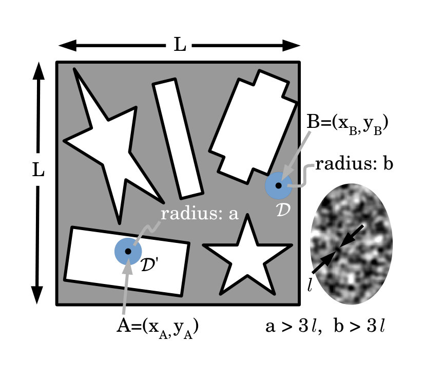 Figure 1
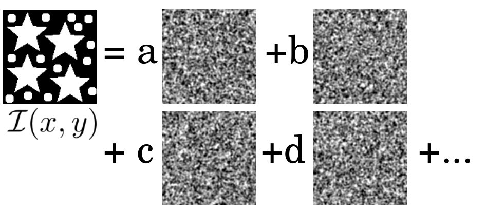 Figure 2
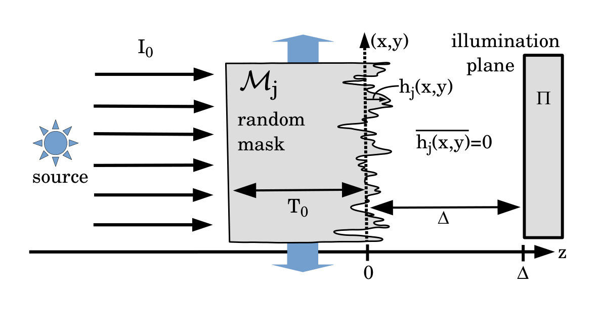 Figure 3
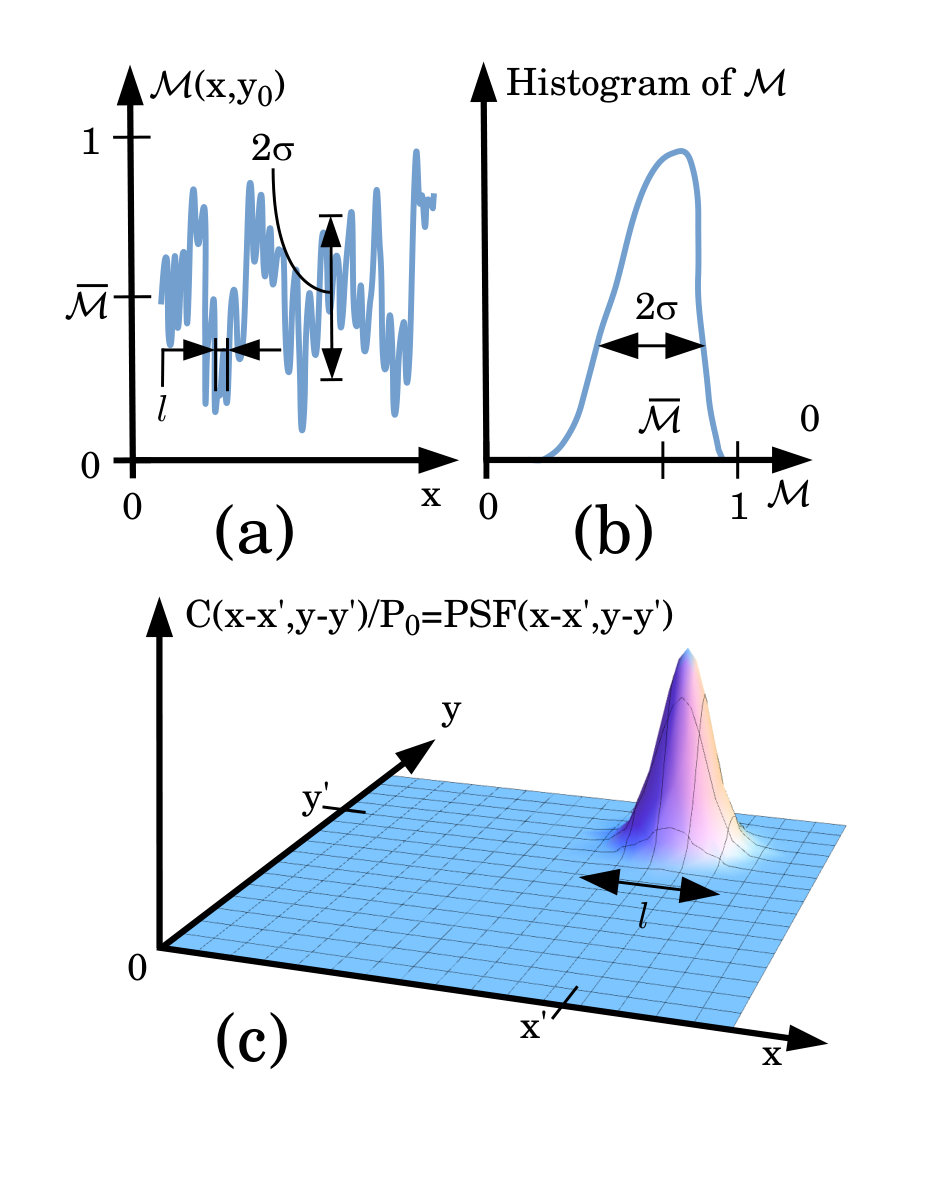 Figure 4
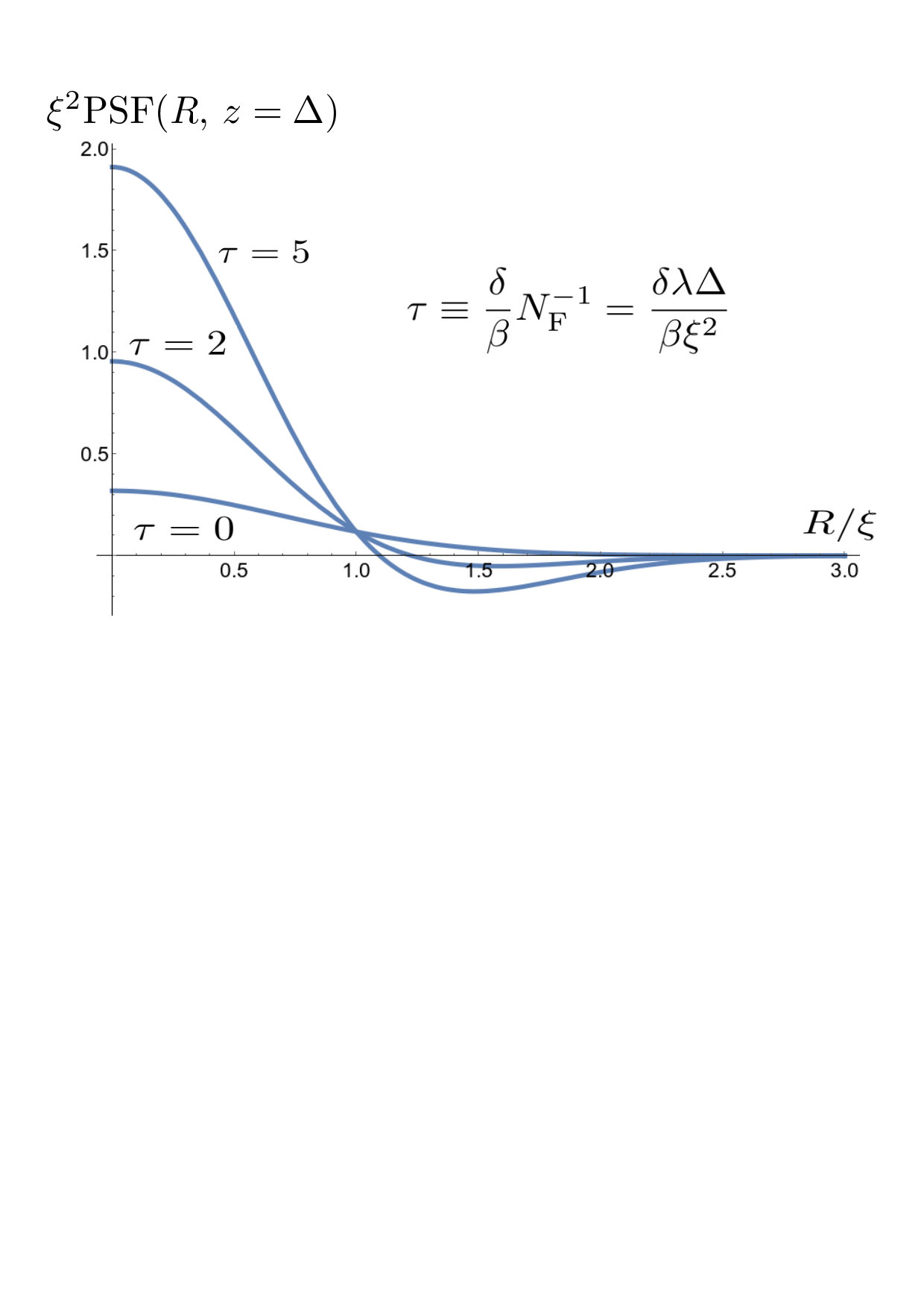 Figure 5
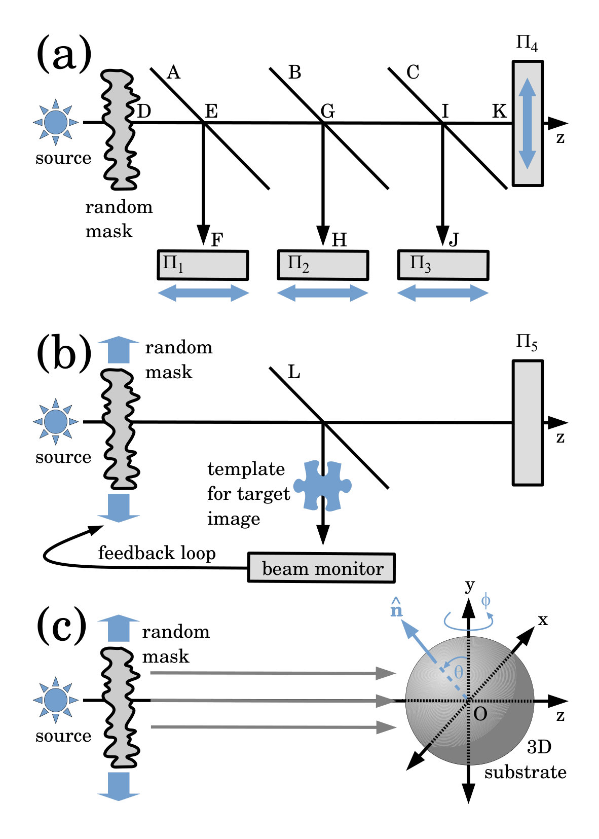 Figure 6
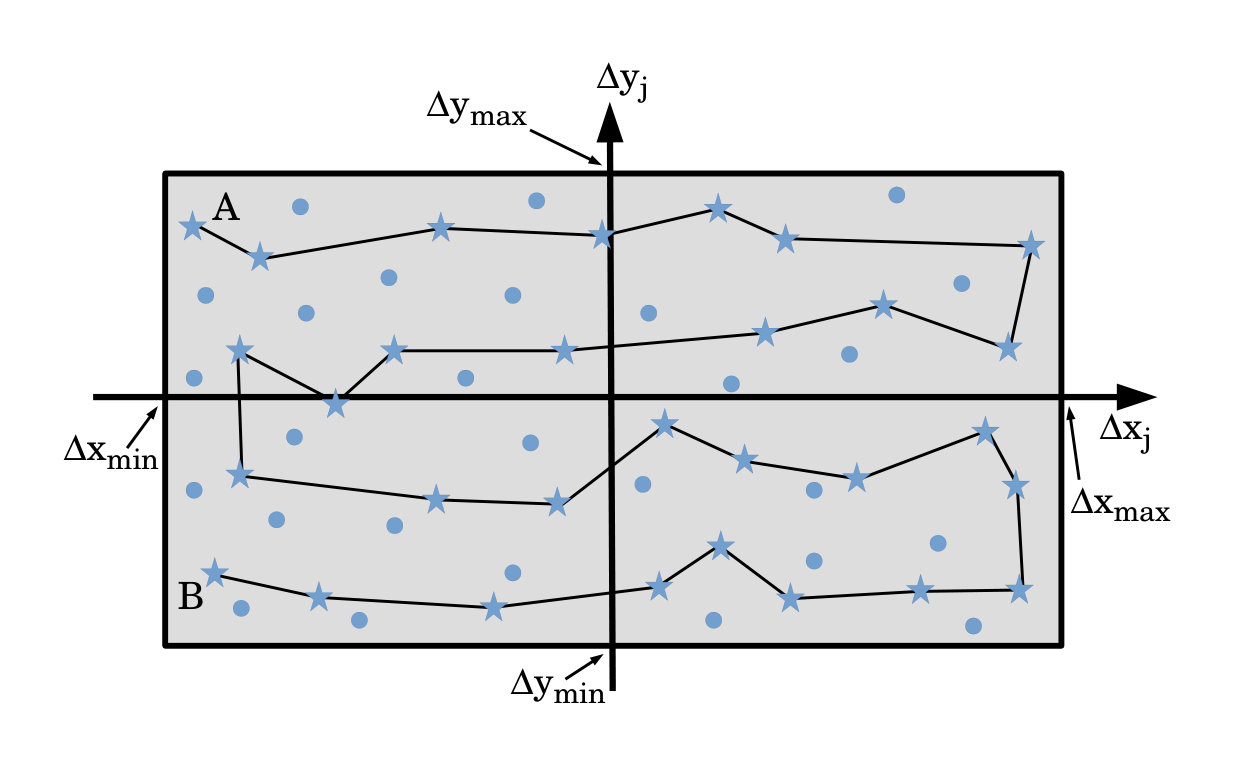 Figure 7
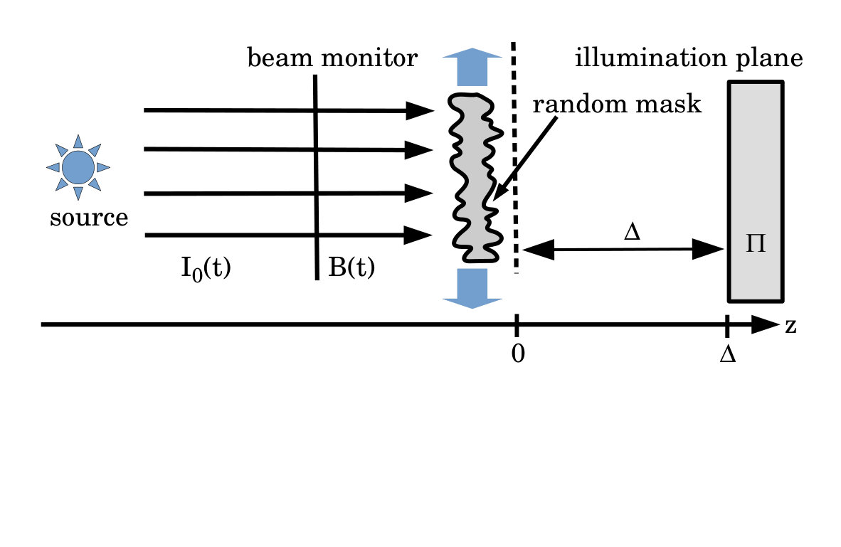 Figure 8
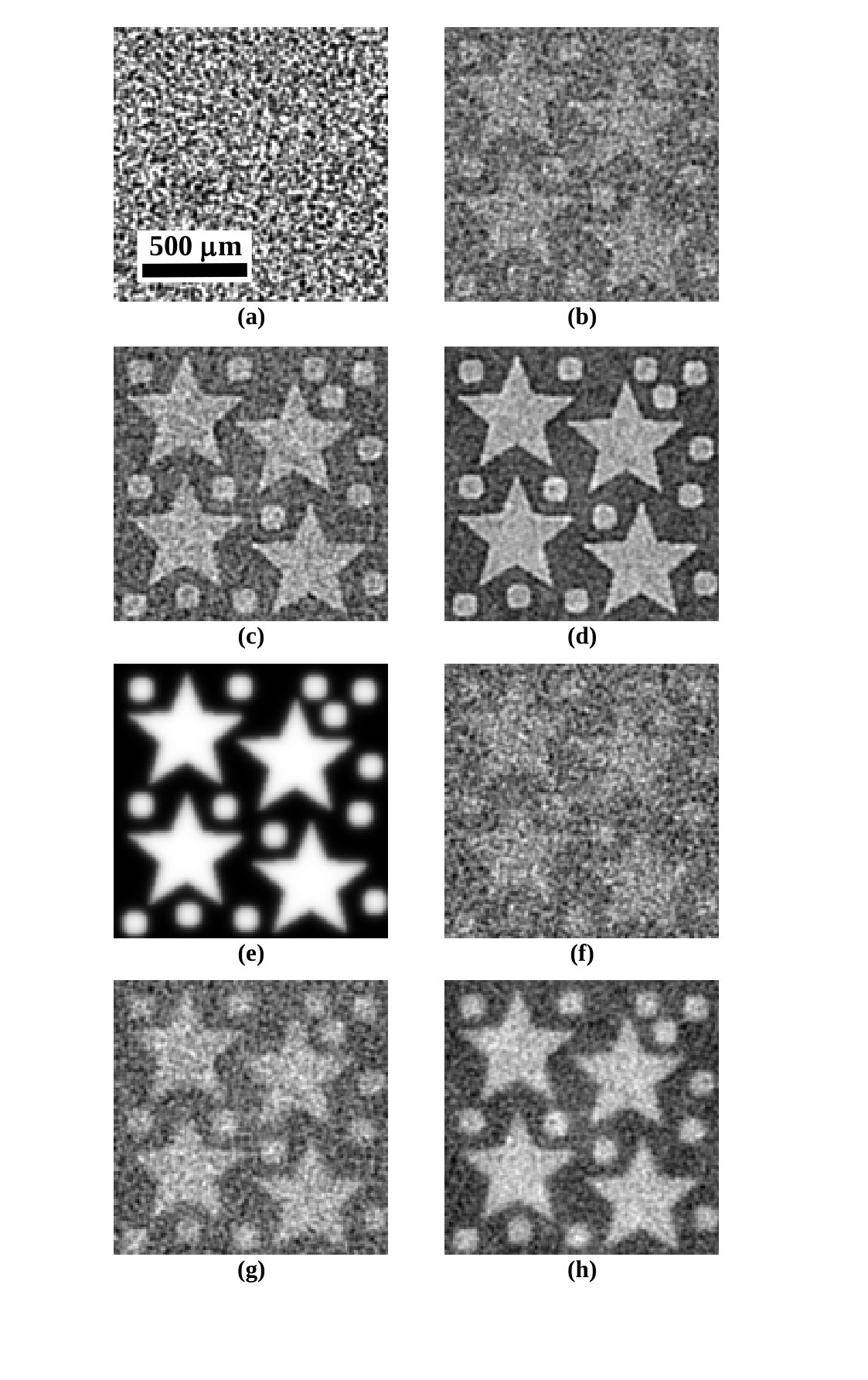 Figure 9
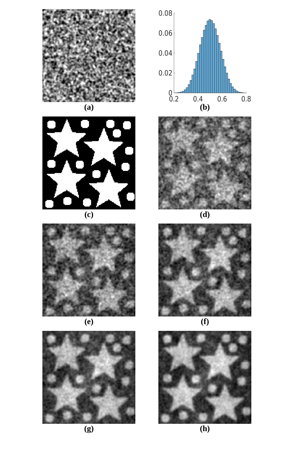 Figure 10
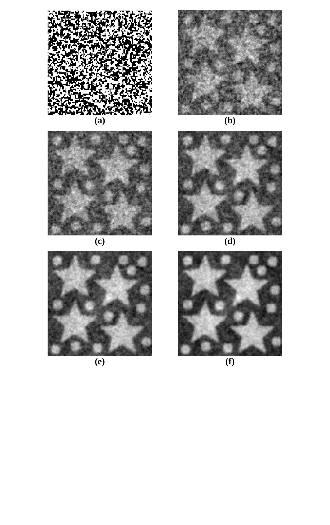 Figure 11
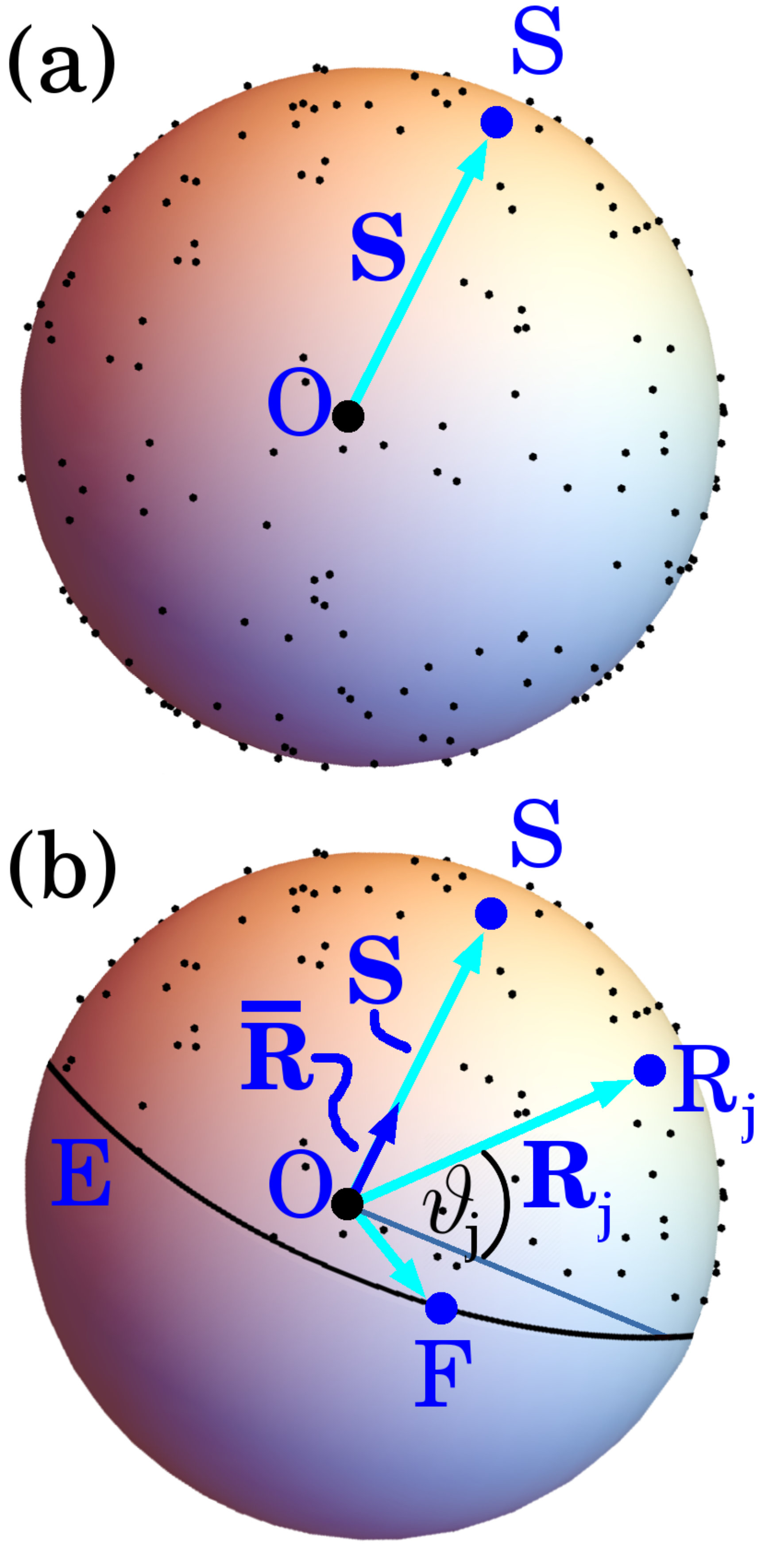 Figure 12
Peer Reviews
No public reviews on file for this paper yet. If you reviewed it on a platform where reviews are public (OpenReview, ICLR, NeurIPS, ICML), you can paste yours below so the community can read it here.
Videos
No videos yet. Explain this paper in a talk, walkthrough, or lecture? Add one.
One mask to rule them all: Writing arbitrary distributions of radiant exposure by scanning a single illuminated spatially-random screen
David M. Paganin
School of Physics and Astronomy, Monash University, Victoria 3800, Australia
Abstract
Arbitrary distributions of radiant exposure may be written by transversely scanning a single known spatially-random screen that is normally illuminated by spatially but not necessarily temporally uniform radiation or matter wave fields. The arbitrariness, of the written pattern of radiant exposure, holds up to both (i) a spatial resolution that is dictated by the characteristic transverse length scale of the illuminated spatially random screen, and (ii) a background term that grows linearly with the number of random-illumination patterns. Two classes of the method are developed. The former assumes the distance between the illuminated random mask and the target plane to be sufficiently small that the effects of diffraction may be neglected. The latter accounts for the effects of Fresnel diffraction in the regime of large Fresnel number. Numerical simulations are provided for both variants of the method. Contrast and signal-to-noise ratio are also considered. The method may be parallelized, and is suited to both magnifying and de-magnifying geometries. Possible applications include spatial light modulators and intensity projectors for those matter and radiation wave fields for which such devices do not exist, printing or micro-fabrication in both two and three spatial dimensions, and lithography.
I Introduction
Synthesis and decomposition, of the functions used to model physical systems, often employs weighted superpositions of elements drawn from complete sets of basis functions Gureyev et al. (2018). Completeness holds irrespective of whether the problem under consideration is linear or non-linear. Basis-function sets may be localized or delocalized, depending on whether or not their support (or essential support) coincides with the entire volume under consideration, or some compact subset thereof. Localized bases include the Dirac-delta basis Messiah (1961), wavelet bases Mallat (2009), the pixel basis Hsieh et al. (1996), tight-binding basis functions Ashcroft and Mermin (1976) etc. Polynomial bases Spencer (2016), the Fourier basis Bracewell (1986), the Bloch-wave basis Cowley (1995), the Hermite–Gauss basis Saleh and Teich (2007), multipole-expansion bases Jackson (1999), Green-function and other propagator-based constructs Strauss (1992) all exemplify bases that are delocalized.
Another criterion for classifying complete bases, in the context of using them to construct functions that model physical systems, is the distinction between deterministic and random bases Ceddia and Paganin (2018). The previously-listed bases are all deterministic, as indeed are the majority of bases in common use. This is related to the systematic manner in which such bases are constructed, e.g. using standard approaches to solving key differential equations of mathematical physics Tikhonov and Samarskii (1963): modal approaches Garanovich et al. (2012), eigenfunction expansions Zhidkov (2009), approaches that exploit symmetries Stephani (1989), multi-scale expansions Gao and Xing (2017) etc. Many but not all deterministic bases admit a natural ordering, e.g. via increasing eigenvalue, increasing modal order, increasing energy, increasing magnitude of momentum, increasing characteristic spatial or temporal scale etc.
All of the above is of course extremely well known. Focus attention, then, on random basis functions Akhavi et al. (2009); Vempala (2004). This may be motivated by the idea that randomly-chosen vectors, in a suitable function space, will typically be linearly independent and may therefore be considered as a basis Gorban et al. (2016). Lack of orthogonality may be replaced with the weaker notion of orthogonality in expectation value Ceddia and Paganin (2018) for random bases that become over-complete as sufficiently more members are added Nakanishi-Ohno et al. (2016). The ordering of elements in a random basis, e.g. of random vectors in the -dimensional vector space , may not be particularly meaningful even when it can be readily achieved e.g. by sorting the basis vectors in order of increasing norm. If all elements of a random basis are generated by the same stochastic process, each basis member is in some sense statistically equivalent, therefore if enough such members are generated the set will become over-complete. The property of over-completeness is not peculiar to random bases, as the well-known over-completeness of the coherent states (eigenfunctions of the destruction operator) shows Mandel and Wolf (1995). Convergence rates, for random-basis expansions consisting of terms, are often on the order of in the -norm Gorban et al. (2016). As with all truncated expansions, there is a trade-off between the expense of using a large number of terms to accurately represent a function in a random-basis-function expansion, versus the increased error inherent in using fewer terms Nakanishi-Ohno et al. (2016).
Random bases are used in many fields of physics. For example, sequences of random orthonormal Hilbert space bases are used in the study of quantum chaos Zelditch (2014). Both ghost imaging Klyshko (1988); Bromberg et al. (2009); Katz et al. (2009); Erkmen and Shapiro (2010); Shapiro and Boyd (2012); Padgett and Boyd (2017) and single-pixel cameras Duarte et al. (2008); Sun et al. (2016); Rousset et al. (2017), when utilizing spatially random speckle fields, rely strongly on the random-basis concept Katz et al. (2009); Bromberg et al. (2009); Ceddia and Paganin (2018); Gureyev et al. (2018). The field of compressed sensing Candès and Tao (2006) utilizes random bases in a rich variety of applications both within and beyond physics: see e.g. the review by Rani et al. Rani et al. (2018) and references therein. Extensions beyond strictly physics-based applications include the use of random projections for databases Achlioptas (2003), facial recognition Chawla and Bowyer (2005), machine learning Gorban et al. (2016), neural networks Vempala (2004) and control theory Gorban et al. (2016).
Compressive sensing (albeit of a sparse or compressible signal) may be spoken of as “signal recovery from random projections” Candès and Tao (2006). A variation on this theme, namely the question of signal synthesis using random projections, is the key topic of the present paper. In our context, the idea is illustrated in Fig. 1. Here, we seek to express a specified radiant-exposure distribution as a linear combination of two-dimensional (2D) speckle maps. Each of these speckle maps is by assumption a different realization of a single spatially stationary ergodic stochastic process, such that (i) the mean and variance of the intensity are independent of position, and (ii) the intensity covariance is dependent only on coordinate differences 111As shall be seen, it is convenient to work with a less general stochastic process, in which an ensemble of speckle maps is generated by taking a single two-dimensional speckle map and displacing it by random amounts in both transverse directions.. This last-mentioned condition is equivalent to the statement that the characteristic transverse speckle size is independent of position in the field of view. The resolution of the resulting random-basis synthesis of will hold up to a spatial resolution governed by the speckle size Ferri et al. (2010); Pelliccia et al. (2018); Gureyev et al. (2018), if enough elements are superposed.
Many motivations exist for pursuing optical schemes able to write arbitrary specified patterns via transverse scanning of a single illuminated spatially-random mask. This is a means for creating spatial light modulators (SLMs) for those radiation and matter wave fields, for which SLMs (i) do not exist, (ii) are prohibitively expensive, or (iii) do not have sufficiently high spatial resolution. Examples include the hard x-ray regime, as well as neutron beams, muon beams and atomic beams. Reduced cost and complexity are another motivation, since compared to an SLM or data projector, the method is able to generate desired patterns using only a steady source, a transversely scanned random screen, and an illumination plane/substrate. Other potential applications include lithography and three-dimensional (3D) printing.
We close this introduction with a brief overview of the remainder of the paper. Section II develops the underpinning theory of scanning a single known two-dimensional spatially random mask, that is illuminated by a spatially but not necessarily temporally uniform beam, so as to write an arbitrary specified pattern of radiant exposure over a plane downstream of the illuminated mask. We firstly consider the case where the distance from the mask to the illumination plane is sufficiently small that the effects of diffraction may be neglected (Sec. II.1). We then give a means by which such diffraction effects may be accounted for, provided certain specified conditions are met (Secs. II.2 and II.3). In all of these first three sub-sections of Sec. II, the topic of resolution emerges naturally, via the association of the effective point spread function (by which the synthesized pattern of radiant exposure is smeared) with the auto-covariance of the speckles from which such patterns are synthesized (cf. Fig. 1). This consideration of the resolution of the method is then augmented with Sec. II.4, which considers contrast and signal-to-noise ratio. The theory of Sec. II is illustrated with numerical simulations in Sec. III. Section IV gives an underpinning geometric picture. A discussion, including possible future applications and extensions of the method, is given in Sec. V. We conclude with Sec. VI.
II Theory
Consider a spatially random mask with known intensity transmission function that is a spatially stationary, ergodic, isotropic, stochastic function of transverse coordinates and . The mask transverse dimensions are assumed to be large with respect to the characteristic transverse length scale of the speckled intensity distributions that arise over the exit surface of the mask, when uniformly illuminated by normally-incident statistically stationary partially coherent radiation or matter waves. Spatial stationarity implies to be independent of , while the added assumption of implies (i) spatial averages may be interchanged with ensemble averages; (ii) the statistical properties of the mask are independent of the origin of coordinates. Since ensemble and spatial averages are equal, both will be denoted by an overline, and used interchangeably.
Consider Fig. 2. Here, a statistically stationary source (e.g. of photons, neutrons, electrons, muons, pions, alpha particles, etc.) with intensity , uniformly illuminates a beam monitor that generates a signal
[TABLE]
where is a real constant and denotes time. The illumination need not be mono-energetic, and its intensity may fluctuate with time, but it is assumed to be both spatially uniform and parallel to the optic axis .
At the exit surface of the spatially random mask, which has intensity transmission function with respect to the energy spectrum of the illuminating particles or fields, the intensity distribution will be
[TABLE]
Here, we have introduced time-dependent transverse shifts and in the and directions, respectively. Below it is shown how the exposure time for each transverse shift may be chosen so that the time-integrated intensity (and hence the radiant exposure), over the illumination plane , can have any specified distribution (up to resolution , and a background term that grows linearly with the number of patterns).
Consider the set of spatially random patterns:
[TABLE]
where is a sequence of transverse displacement vectors, which are such that the distance between any two of these displacements is no smaller than the speckle size :
[TABLE]
Here denotes the Euclidean norm of a 2D vector, and . The condition in Eq. (4) ensures the masks in Eq. (3) are linearly independent. A cross-section through one realization of is sketched in Fig. 3(a), indicating the mean value , characteristic speckle size , and standard deviation in the transmission function. See also Fig. 3(b), which sketches a histogram of the mask transmission function. Note for later reference that we denote the mask with transmission function by .
The auto-covariance of the ensemble of masks in Eq. (3), which spatial stationarity implies to be a function only of coordinate differences, is estimated via:
[TABLE]
Here, and are any pair of points in the mask domain , and should be sufficiently large that the right side of Eq. (5) is indeed a good estimate for . This auto-covariance will typically be a peaked function that decays to zero, which isotropy implies to be rotationally symmetric, with diameter given by the speckle size of the random mask. See Fig. 3(c).
Let the normalization constant be defined by
[TABLE]
which will be independent of on account of spatial stationarity. Now, has the properties expected for a point-spread function (PSF): it is narrow and peaked, with an area of unity Hecht (1998). Hence let
[TABLE]
so that Eq. (5) becomes a smoothed completeness relation 222Equation (8) is spoken of as a “smoothed completeness relation” on account of its direct comparison with the completeness relation (closure relation) Gureyev et al. (2018); Bransden and Joachain (1989). Here, each member of a complete complex basis is denoted by , are position vectors and denotes the Dirac delta. Dropping the star due to working with real functions, truncating the sum to a finite number of terms , and replacing the Dirac delta with a mollified (smoothed) form that is nonetheless both peaked and normalized to unity, leads directly to Eq. (8). Here, the background-subtracted mask functions play the role of a random set of basis functions that are orthogonal in expectation value Ceddia and Paganin (2018); Pelliccia et al. (2018):
[TABLE]
Now let be a desired distribution of radiant exposure over the surface of the plane in Fig. 2. We separately consider the case where: (i) ; (ii) .
II.1 Case #1:
Multiply both sides of Eq. (8) by , then integrate over and , to give:
[TABLE]
Here denotes two-dimensional convolution,
[TABLE]
is the inner product (cross correlation) of the the th random mask with the desired radiant-exposure distribution , and:
[TABLE]
To proceed further, observe that
[TABLE]
Hence the term may be dropped from Eq. (9). This leaves a formula that is familiar from the different but related context of classical ghost imaging Bromberg et al. (2009); Katz et al. (2009); Pelliccia et al. (2018); Gureyev et al. (2018):
[TABLE]
This random-basis expansion expresses the desired radiant-exposure distribution , up to a resolution of implied by PSF smearing, as a linear combination of transversely displaced masks in Eq. (3) (cf. Fig. 1).
In a ghost-imaging context Padgett and Boyd (2017), would be measured “bucket signals” that may be used to reconstruct a ghost image of the left side of Eq. (13). In our context, we wish to synthesize the left side of Eq. (13) by calculating the required coefficients using Eq. (10) and then exposing each known mask for a time proportional to . However, there is an important difference between the ghost-imaging application of Eq. (13), and the pattern-writing application we consider: is a zero-mean random variable that can take on both negative and positive values. This conflicts with the fact that the exposure time for the th mask, which should be proportional to , cannot be negative.
Hence adopt the following process:
Randomly select a set of mask translation vectors , which lie within the maximum range specified by and (see Fig. 4).
Calculate for each translation vector using Eq. (10), and hence calculate using Eq. (11). 3. 3.
Reject all translation vectors for which (rejected vectors are marked as discs in Fig. 4, with accepted vectors as stars). This amounts to keeping only mask positions for which has a cross correlation with the desired pattern that is larger than the average cross correlation. 4. 4.
Approximately translation vectors will remain, with to ensure the spacing between translation vectors is greater than , where . Join these together with an efficient path, giving the sequence of mask translations shown in Fig. 4. Note that, by construction, for each of these masks. 5. 5.
If the spatially uniform incident illumination (see Fig. 2) is independent of time , expose each mask for a time proportional to : thus , where is a constant. If the spatially uniform incident illumination varies with time, as measured by the beam monitor in Eq. (1), expose each mask for a time such that the total transmission is proportional to .
With the above steps, and provided is sufficiently large, Eq. (13) implies that the distribution of radiant exposure, over the plane in Fig. 2, will be equal to the required distribution . This equality will hold up to (i) a multiplicative constant; (ii) isotropic transverse smearing over a length scale of , due to the rotationally symmetric PSF associated with the process; (iii) a background term that grows linearly with the number of patterns, that is a consequence of Step #3 above. This last-mentioned property is an important limitation of the method, whose resulting radiant exposure may be written as
[TABLE]
Here, is a constant for the case where the incident illumination intensity is independent of time.
II.2 Case #2:
Now consider the case where in Fig. 2 is sufficiently large that the effect of free-space diffraction cannot be ignored, due to propagation between the exit surface of the mask and the target surface .
Introduce additional assumptions that enable modelling of this free-space diffraction process: (i) Assume the illumination to be a quasi-monochromatic complex scalar field Born and Wolf (1999), which for concreteness we take to be hard x rays. (ii) Assume both mask and illumination to be such that the projection approximation is valid Paganin (2006). This is a high-energy approximation that amounts to assuming the mask to be sufficiently slowly varying, and the illumination of sufficiently high energy, that the streamlines of the current density within the mask are very close to parallel to the optic axis. (iii) Assume the mask to be made of a single material with linear attenuation coefficient , and real refractive index Paganin (2006). (iv) Assume the Fresnel number
[TABLE]
corresponding to Fresnel diffraction of paraxial waves with wavelength , to obey
[TABLE]
Stated differently, assume is small enough that the plane is in the near field of the spatially random mask Paganin (2006) (see Fig. 2). (v) Assume the incident illumination intensity to be time-independent. This last assumption is easily dropped, but has been included for both simplicity and clarity.
The above assumptions enable use of a finite-difference form of the transport-of-intensity equation Teague (1983), namely the continuity equation expressing local energy conservation for the parabolic equation of paraxial wave optics Paganin and Pelliccia (2019). This gives the following estimate for the intensity distribution, due to illumination of the th state of the mask, over the target surface in Fig. 2 Paganin et al. (2002):
[TABLE]
Here, is the Laplacian in the plane, the projected thickness of the th state of the mask is:
[TABLE]
is a constant offset mask thickness and is a stochastic fluctuation that (i) ensemble averages to zero at every point in the domain of the mask; (ii) spatially averages to zero for every realization of the mask (see Fig. 5). Note that the projected thickness in Eq. (18) may be produced by either or both of (i) surface roughness and (ii) density fluctuations within the mask. The former case is illustrated in Fig. 5.
Now assume the absorption of the mask to be weak, so that the exponential in Eq. (17) can be Taylor expanded to first order in its argument. To first order in , this gives the following expression for the auto-covariance of the intensity illuminating the target plane :
[TABLE]
Here,
[TABLE]
Note that Eq. (20) makes the intuitive statement that Fresnel diffraction does not change the average transverse energy density of the propagating radiation. Note also, that the Laplacian in Eq. (19) acts only on the coordinate, and not on .
Denote the illuminating-intensity auto-covariance by
[TABLE]
and the height auto-covariance by
[TABLE]
where the last equality follows from . Upon transforming from Cartesian coordinates to plane polar coordinates , and dropping explicit dependence due to rotational symmetry, Eq. (19) becomes:
[TABLE]
As was the case in Sec. II.1, promote the intensity covariance to the status of a PSF for the corresponding distribution of radiant exposure, by normalizing to unity using Eq. (7). Thus
[TABLE]
where the -independent normalization constant
[TABLE]
ensures that for all . Note that a boundary term has been discarded in deriving Eq. (25), by applying the Gauss divergence theorem to and assuming that decays to zero faster than . Thus Eq. (23) becomes:
[TABLE]
By comparing the case of Eq. (26) with the case for , where is the largest mask-to-target-plane propagation distance consistent with the key assumption that the Fresnel number be much larger than unity, we see that
[TABLE]
Here, is the linear differential operator:
[TABLE]
Note that operators will always be considered to act on all objects that appear to their right, so that e.g.
[TABLE]
for operators and functions . Note also that the Fourier derivative theorem gives the following Fourier representation for Paganin et al. (2002); Paganin (2006)
[TABLE]
where denotes Fourier transformation with respect to , denotes the corresponding inverse Fourier transformation, and are Fourier variables dual to . We have used a Fourier-transform convention in which the Fourier derivative theorem takes the form where differentiation with respect to or in space corresponds to multiplication by or in space. In this Fourier representation, the inverse to is the Lorentzian low-pass Fourier filter
[TABLE]
A convolution representation of is readily obtained, with the aid of both the convolution theorem of Fourier analysis and a table of Hankel transforms Bracewell (1986). Hence:
[TABLE]
Here, is the modified Bessel function of the second kind and zeroth order.
Next, recall the fact that the definition of the convolution integral implies
[TABLE]
for any linear operator and any functions that are sufficiently well behaved that the orders of application of (i) integration and (ii) can be interchanged. Now, if we were to use in the scheme outlined in the previous sub-section, which neglects the effects of non-zero , Eq. (13) shows that the target plane would register a radiant-exposure distribution that is proportional to . Making use of Eqs. (27) and (33) and reverting back to Cartesian coordinates, we see that (up to the previously mentioned proportionality) this registered radiant-exposure distribution may be written as:
[TABLE]
The presence of in the final line of Eq. (34) implies that the wrong pattern will be written, if we were to apply the scheme of Sec. II.1 without modification: up to smearing by , the pattern that is written is rather than the required pattern of .
The required modification is to make the replacement
[TABLE]
in Eq. (34), to obtain
[TABLE]
This is the key result of the present sub-section, since the last line of Eq. (36) is the required pattern , smeared by the “contact” PSF.
Hence, when in Fig. 2 is large enough that its effects cannot be neglected, we can obtain a desired radiant-exposure distribution over the target plane using the setup in Fig. 2, with exactly the same sequence of five steps in Sec. II.1, via the single modification that the replacement in Eq. (35) is made. Note that, in the limit , we have , so that the formalism of the present sub-section is a generalization of that in Sec. II.1.
We close this sub-section by noting the asymptotic behavior (see e.g. Eq. (10.25.3) in Olver et al. Olver et al. (2010))
[TABLE]
of the convolution kernel in Eq. (32). This exponential decay ensures that, when acts on a compactly supported distribution such as the desired target pattern , the result is also compactly supported.
II.3 Remark
Many models for rough surfaces, such as that of Sinha et al. Sinha et al. (1988), could be introduced for and in Sec. II.2. For simplicity, consider the Gaussian form
[TABLE]
Here, is the variance of the height distribution sketched in Fig. 5 (see also Eq. (18)), and is the characteristic transverse length scale over which the rough height profile is correlated. The same quantity is equal to the characteristic transverse speckle size for any particular realization of Eq. (17). It is also equal to the spatial resolution with which the scheme of the present paper allows the desired pattern to be written.
For the model in Eq. (38), Eq. (26) becomes the family of normalized PSF curves:
[TABLE]
Here, , where is the wave-number corresponding to vacuum wavelength , and the Fresnel number is .
Three different instances of these PSFs are sketched in Fig. 6, corresponding to three different values for the dimensionless parameter
[TABLE]
When , corresponding to , we have a Gaussian PSF. However, when , the central positive peak in the PSF develops a negative “moat” due to Fresnel diffraction through the distance . Note that the choice of non-zero values illustrated in Fig. 6 has been guided by the facts that (i) the Fresnel number must be much greater than unity for Eq. (17) to be valid; (ii) typical values for are in the range of for many materials in the hard x-ray regime. The “moats” evident in the PSFs of Fig. 6, which are a special case of similar behavior for the more general expression in Eq. (27), are consistent with similar features seen in several papers calculating experimental x-ray speckle correlation functions in a different context, namely x-ray phase contrast velocimetry Irvine et al. (2008, 2010a); Ng et al. (2012).
II.4 Contrast and signal-to-noise ratio
The resolution inherent to the method has arisen naturally in Secs. II.1–II.3, due to the connection between this function and the speckle–speckle auto-covariance. We supplement this by considering the complementary attributes of contrast and signal-to-noise ratio (SNR). In Sec. II.4.1 we first consider the contrast and SNR associated with the pre-truncation basis, namely Eq. (13) prior to the rejection of the terms with . This gives a “base case” for comparison, which is directly related to a commonly-used method in the different but related context of ghost imaging Katz et al. (2009); Bromberg et al. (2009). Section II.4.2 then considers the truncated basis central to this paper, namely the modified form of Eq. (13) given in Eq. (14). Expressions are given for both the contrast and the SNR.
II.4.1 Contrast and signal-to-noise ratio: Non-truncated basis
Let the target distribution of radiant exposure be binary, taking on the values of either zero or unity, over a square region with physical dimensions square meters. See Fig. 7. Let be the fraction of the area for which . The auto-covariance in Eq. (5) will have a diameter of approximately the diameter of the speckles. The peak value of this covariance will be the variance
[TABLE]
where is the standard deviation of the intensity of the illuminating speckle masks (see Fig. 3). Since has a peak value of and a diameter of , the normalization constant in Eq. (6) obeys:
[TABLE]
Now consider a point that is well within the target’s background in the sense that there is a disk of radius centered upon , with for all . Stated differently, the shortest distance from to any interface in the binary pattern , is such that (see Fig. 7). Since vanishes at every point in the disk centered at the background point , the calculation of the coefficients in Eq. (10) will contain no information regarding the speckles of that overlap . This implies that the random variables and , which appear as a product in the summand of Eq. (13), are statistically independent. Note also that we consider the result of applying Eq. (13) to one particular realization of speckle fields, as itself being a random variable. Denoting the expectation of this random variable via , we obtain the following for a “background point” :
[TABLE]
Note that: (i) We have used the linearity of expectation values in passing from the second to the third lines of Eq. (43); (ii) We have used the statistical independence of the random variables and , in passing from the third to the fourth lines; (iii) We see from Eq. (43) that the expectation value at a point that is “deep within the background region” where vanishes, will itself vanish, thus the average at indeed converges to , as expected; (iv) Eq. (43) is unphysical insofar as it incorporates negative exposure times.
Next, we calculate the variance of the random variable . Aspects of the remainder of this sub-section use techniques adapted from Gureyev et al. Gureyev et al. (2018) and Ceddia and Paganin Ceddia and Paganin (2018). Equation (13) gives:
[TABLE]
The final line of Eq. (44) contains a product of statistically independent random variables. Recall that, if the random variables and are uncorrelated, with respective means and respective variances , then
[TABLE]
Letting and , and noting that vanishes, Eq. (45) enables Eq. (44) to become:
[TABLE]
To further simplify the right-hand-side of Eq. (46), we require an estimate for . To this end, return to the expression for in Eq. (10). This integral has a discrete approximation corresponding to a sum over the
[TABLE]
speckles (each of area ) contained within the area within which equals unity. Hence the random variable in Eq. (10) is approximately equal to the sum of deviates drawn from a probability distribution with mean and standard deviation . Assuming the contribution to from each speckle to be statistically independent, we can write
[TABLE]
Note that we have used Eq. (47) in obtaining the final equality of Eq. (48). Equation (48) may now be substituted into Eq. (46), and use made of Eq. (42), to give:
[TABLE]
Shift attention to a “foreground” point as shown in Fig. 7. Assume this point to be “well within” the foreground of the target image, in the sense that for all , where is a disk of radius centered upon . From Eq. (13), we have (cf. Eq. (43)):
[TABLE]
However, in contrast to the case in Eq. (43), the random variables and are now correlated. This correlation arises from the fact that speckle-field intensity values —arising from points , including the point —are used in calculating , via Eq. (10). This correlation implies that we cannot equate the right side of Eq. (50) to . Instead, use Eq. (10), which may be substituted into Eq. (50) to give:
[TABLE]
Now note from Eq. (5) that
[TABLE]
where is the previously defined auto-covariance of the ensemble of speckle fields (see Fig. 3(c)). Hence Eq. (51) becomes:
[TABLE]
Since lies within a disk of radius equal to three speckle widths—over all of which is equal to unity, and within which the auto-covariance will have decayed to close to zero—the first double integral in Eq. (53) will be only negligibly changed if is deleted from the integrand. Thus:
[TABLE]
We see from Eq. (54) that the average at indeed converges to , as expected.
The preceding calculations can now be used to determine the contrast and SNR for synthesizing using the non-truncated basis, according to Eq. (13). The contrast converges to unity, on account of Eqs. (43) and (54). The SNR is defined, in the present context, as the following ratio of Michelson-type visibility Michelson (1927) to the standard deviation of the background:
[TABLE]
Equations (43), (49) and (54) then give (cf. Eqs. (15) and (31) in Gureyev et al. Gureyev et al. (2018), together with Eq. (18) in Ceddia and Paganin Ceddia and Paganin (2018)):
[TABLE]
In the second-last line of Eq. (56), we have used Eq. (47). As expected for a random basis Gorban et al. (2016), Eq. (56) grows as the square root of the number of speckle masks . Also, the SNR scales as the inverse square root of . Lastly, the SNR increases linearly with mask contrast 333Equation (57), for the mask visibility, is based on the Michelson visibility formula Michelson (1927). If extreme outliers are excluded by considering the maximum and minimum mask intensities to be and respectively, the mask contrast is then given by Michelson’s formula as .
[TABLE]
II.4.2 Contrast and signal-to-noise ratio: Truncated basis
We now adapt the formulae of the preceding sub-section, to the case where Eq. (13) is truncated to include only those terms for which : see Eq. (14).
For a “background point” as previously defined, Eq. (43) becomes:
[TABLE]
Here, note that: (i) the prime on the sum indicates that terms with have been excluded; (ii) the upper limit on the sum has been changed from to since approximately half of the terms will be discarded from the sum; (iii) statistical independence of and has been used in the final line of Eq. (58), for the sames reasons that were outlined in the previous sub-section, since these reasons still hold in the present context; (iv) the symbol refers to the average of the coefficients before truncation, which is why the final line of Eq. (58) does not vanish.
As mentioned just after Eq. (47), before truncation may be approximated by the sum of deviates drawn from a probability distribution with standard deviation . The central limit theorem then implies that the corresponding probability density will be approximately normally distributed, with variance
[TABLE]
After truncation, the probability density function can be approximated as the half-Gaussian
[TABLE]
where is the Heaviside step function. Thus
[TABLE]
which may be combined with Eq. (42) to write Eq. (58) as
[TABLE]
For the “interior point” , truncation to the half-basis implies that the second-last line of Eq. (54) becomes:
[TABLE]
Truncation to a half-basis implies that the term no longer vanishes. Rather, Eq. (61) implies that
[TABLE]
hence Eq. (63) becomes
[TABLE]
The Michelson contrast in the half-basis, obtained by evaluating the numerator of Eq. (55) using Eqs. (62) and (65), is
[TABLE]
The corresponding SNR is
[TABLE]
We note that the post-truncation SNR is suppressed with respect to the pre-truncation SNR, by the multiplicative factor . This multiplicative factor will be typically smaller—and often much smaller—than unity. Notwithstanding this, the post-truncation SNR grows with the square root of the number of masks, and is proportional to the square of the mask contrast. Hence higher contrast of the illuminating random mask is beneficial. Also, we can always choose the number of masks to be sufficiently large to achieve any target SNR. Conversely, the Michelson contrast of the written pattern has a fixed limit given by Eq. (66), independent of the number of random masks. The maximum attainable contrast, corresponding to 444the upper limit will be fulfilled e.g. by a random binary mask, for which equal areas are assigned 0% and 100% transmission. See Fig. 9(a)., implies that:
[TABLE]
III Simulations
The cases of zero and non-zero (see Fig. 2) are numerically modelled in Secs. III.1 and III.2, respectively.
III.1 Simulations for
To simulate a spatially-random mask, a pixel array is populated with pseudo-random real numbers uniformly distributed between zero and unity. This white-noise array is then smoothed via convolution with a rotationally-symmetric Gaussian with standard deviation equal to one pixel, giving a speckle width of pixels. The resulting random array of gray-scale values is taken to be the continuous-tone transmission function of a mask, denoted by in Eq. (2). A pixel sub-region of this continuous-tone mask is shown in Fig. 8(a), with the corresponding histogram of transmission-level values in Fig. 8(b). The five steps in Sec. II.1 are then followed:
The simulated mask is randomly transversely displaced to different locations, to generate an ensemble of linearly-independent mask transmission functions corresponding to Eq. (3). Each such mask has a field-of-view of pixels, with randomly chosen location within the full pixel mask. For simplicity, periodic boundary conditions are assumed. 2. 2.
The target pattern is taken to be the pixel binary image in Fig. 8(c). Using this motif, is calculated for each translation vector using Eq. (10), with the integral being estimated via addition of pixel values. No transverse length scale needs to be specified in these simulations, hence (i) simulated values are only calculated up to an unspecified multiplicative constant; (ii) there are no spatial scale bars in Fig. 8. Next, is calculated using Eq. (11). 3. 3.
Rejection of all mask translation vectors for which implies that approximately half of the mask positions are utilized. 4. 4.
For the purposes of simulation, the order in which the masks are exposed is irrelevant, hence there is no need to calculate a suitable trajectory of mask positions such as that shown in Fig. 4. 5. 5.
Each retained mask is multiplied by , corresponding to exposure of the illuminated surface for a time proportional to , under the assumption that is independent of time in Eq. (1). The resulting weighted masks are then summed.
The synthesized radiant-exposure distributions due to mask positions (prior to the rejection of approximately half of the mask positions in Step #3) are shown in Fig. 8(d-h) respectively. The contrast of all synthesized distributions, which is on the order of 1.3%, may be compared to the speckle-mask contrast for the continuous-tone mask, .
The low contrast of the radiant-exposure maps agrees with Eq. (66). To see this, the PSF corresponding to the random mask in Fig. 8(a) was calculated via the auto-covariance in Eq. (7), for which a -pixel block contains most of the PSF area. Hence, making use of the numerical values listed in the caption to Fig. 8, we have , with the corresponding Michelson contrast being given by Eq. (66) as . This is consistent with the simulated contrast, and independent of for large .
To improve the contrast of the radiant exposure, note from Eq. (66) that this contrast is proportional to the contrast of the random mask . Hence we perform an additional simulation, shown in Fig. 9, in which the low-contrast continuous-tone random mask is replaced with a high-contrast random mask. The random binary mask in Fig. 9(a) is simulated using the same process and parameters for the mask in Fig. 8(a), but with an additional step in which the continuous-tone mask is binarized by setting all gray-levels below the median to zero, and all other gray levels to unity. The resulting mask has , which is six times larger than the value of for the continuous-tone mask. Hence Eq. (66) predicts a six-fold increase in the contrast of the radiant exposure, i.e. an increase from 1% to 6%. This prediction of Eq. (66) is consistent with the simulations shown in Figs. 9(b-e), which show the contrast converging to 6.4%.
III.2 Simulations for
Consider a spatially random mask made from a copper sheet with one roughened surface (see Fig. 5). The following simulations assume this to be illuminated by normally incident quasi-monochromatic x rays of energy 17.2 keV (wavelength 0.72 Å). The corresponding optical parameters are and Gureyev et al. (2002). Assume a characteristic transverse length scale for the roughness of m. Since the Fresnel number must be much greater than unity for our analysis to be valid, set in Eq. (15) and solve for the mask-to-substrate distance to give m. This distance is reasonable and practical for synchrotron and laboratory sources of hard x rays. Setting the aspect ratio of the roughness to 0.05 estimates the standard deviation of the stochastic height profile to be approximately m (cf. Eq. (38)). The same “filtered white noise” approach, as in Sec. III.1, is used to simulate one spatially random mask with projected thickness consistent with the above parameters (see Eq. (18)). A pixel array is again used for the entire random mask, with the same pixel target distribution as in Fig. 8(c). The physical width and height of each pixel are 10 m. The mask substrate thickness does not need to be specified since it only affects all outputs by a multiplicative constant.
The projection approximation Paganin et al. (2002); Paganin (2006) is used to calculate the complex x-ray wave field at the exit surface of the mask, as a function of the modelled projected thickness, using the parameters given above. The Fourier representation of the Fresnel propagator is then used to calculate the propagated intensity over the target plane, due to each mask. The propagated speckle field for one position of the mask, corresponding to m in Fig. 2, is shown in Fig. 10(a). Compared to the non-propagated speckle in Fig. 8(a), Fig. 10(a) has additional fine detail due to propagation-based phase contrast Snigirev et al. (1995); Cloetens et al. (1996); Wilkins et al. (2014) as quantified by the Laplacian term in Eq. (17). When no correction is made for the non-zero , the output maps of radiant exposure in Figs. 10(b-d) are obtained, corresponding respectively to pre-rejection mask positions. The high-pass filtration of by , as predicted in Eqs. (30) and (34), is evident as the black-white halos at the edges of each feature in the patterns of radiant exposure, together with the fact that the background is paler than was the case in Fig. 8. Such halos may also be thought of as due to the “moat” surrounding the PSFs in Fig. 6. Notwithstanding these distortions, Figs. 10(b,c,d) look sharper than their counterparts in Figs. 8(d,e,h), since Eq. (17) is mathematically identical in form to Laplacian based unsharp-mask image sharpening Easton Jr (2010); Brown et al. (2013), albeit in an over-sharpened regime where the previously mentioned black-white halo surrounds feature edges. To correct for the formation of such artefacts, is transformed according to the replacement given in Eq. (35), using the convolution representation (Eq. (32)) of the smoothing operator . The characteristic transverse length scale for the modified Bessel function smoothing kernel is obtained from the previously stated values of to be pixels (cf. Eq. (32)). The result, namely , is shown in Fig. 10(e). The corresponding maps of radiant exposure in Figs. 10(f-h), which correspond to pre-rejection masks respectively, are not distorted by a black-white halo. Note that, while there may appear to be a faint remaining halo when inspecting Figs. 10(f-h), this is not in fact that case, but is rather due to the Mach band phenomenon of physiological optics Eagleman (2001); Wallis and Georgeson (2010).
IV Underpinning geometric construction
Suppose we wish to construct a particular vector connecting the center of a unit sphere to an arbitrary specified point on the surface of that sphere, using a method of construction that employs only random unit vectors as a basis. See Fig. 11. Below we consider this construction for the unit-radius -sphere (Sec. IV A) and the unit-radius -sphere (Sec. IV B). We explain how this gives an underpinning geometric construction that clarifies several key results of the present paper (Sec. IV C), as well as leading to some additional results (Sec. IV D).
IV.1 Unit-radius 2-sphere
As shown in Fig. 11(a), cover the unit 2-sphere with uniformly distributed random points , , with each of which is associated a vector connecting the center of the sphere to the th random point . Arbitrarily denote to be the pole of the unit 2-sphere, with associated equator and equatorial points such as : see Fig. 11(b). Keep only those random vectors for which lies in the hemisphere containing ; there will be approximately such vectors, if is large. Average these random vectors to obtain a vector , which is itself a random variable, whose expectation value will be parallel to :
[TABLE]
More precisely,
[TABLE]
where the final equality follows from spherical symmetry, together with the fact that is a unit vector. The correlation coefficient
[TABLE]
is the averaged projection onto the axis defined by the specified point . Since this correlation coefficient is a function of the dimensionality of the sphere, and we are here considering a 2-sphere, a subscript of 2 has been placed on this correlation. Hence
[TABLE]
This shows that the average of the random unit vectors that lie in the hemisphere having the specified point as a pole, when divided by the correlation coefficient , will have an expectation value of . Equation (72) completes our geometric construction of a desired unit vector, given an ensemble of unit vectors with random directions in three spatial dimensions.
IV.2 Unit-radius -sphere
For the unit-radius -sphere embedded in spatial dimensions, Eq. (72) generalizes to:
[TABLE]
provided that the only random vectors that are kept are those that lie in the hemisphere containing as its pole. Assuming that , the concentration-of-measure property of high-dimensional spheres implies the overwhelming majority of random vectors to be concentrated in the vicinity of any equator Ledoux (2001); Sethna (2006); Qiu and Wicks (2014). If we introduce the latitude angle
[TABLE]
for the random unit vector , this concentration property implies that the corresponding probability density will be a normal distribution with mean zero and variance that is inversely proportional to the dimensionality of the hyper-sphere Sethna (2006):
[TABLE]
However, we have by construction deleted all random vectors that have a negative correlation with the specified vector (negative projection , and hence a negative ). Hence, for large dimension the probability density will correspond to the truncated normal distribution (cf. Eq. (60)):
[TABLE]
Here, the breve denotes a quantity associated with the truncated distribution, with an absence of a breve denoting a pre-truncation quantity. Prior to truncation, the mean and variance of the density are equal to and respectively. Post-truncation, we can use Eq. (76) to obtain:
[TABLE]
The correlation coefficient appearing in Eq. (73) is obtained via the -dimensional generalization of Eq. (71):
[TABLE]
Hence Eq. (73) becomes:
[TABLE]
More generally, spherical symmetry implies that
[TABLE]
where is (i) any weight function of non-negative latitudinal angles if the average is taken oven a hemisphere with pole , or (ii) any non-even weight function of all latitudinal angles if the average is taken over the whole sphere.
IV.3 Geometric interpretation of the method
Equation (47) reveals to be the number of degrees of freedom in Erkmen and Shapiro (2010), since is the number of resolution elements needing to be “switched on” to form a given pattern of radiant exposure. Any particular pattern with “switched on” resolution elements and a specified upper bound on its integrated radiant exposure may be thought of as occupying the surface and interior of a sphere in a function space with dimensions. The concentration property of high-dimensional spheres Sethna (2006) ensures the set of all possible radiant-exposure patterns is represented by a cloud of points over the surface of the -sphere. This connects the purely-geometric construction defined above, to the question of synthesizing desired patterns of radiant exposure using spatially random masks. Under this view, observe that:
- •
A crude form of the method in Sec. IIA keeps steps #1 to #4 unchanged, but uses the same exposure time for each mask in Step #5; this is the direct analog of the geometric construction in Fig. 11(b) (i.e. with ). See Eq. (72).
- •
Alternatively, if each vector in the hemisphere of Fig. 11(b) is first weighted by its correlation coefficient , prior to summing the resulting ensemble of random vectors, we obtain an exact geometric analog for steps #1 to #5 in Sec. II A. This is a geometric version of Eq. (14). Comparing the right sides of Eqs. (68) and (78), upon identifying the hypersphere dimension with , reveals the latter formula to be a geometric distillation of the former.
- •
Suppose each vector in the whole function-space hyper-sphere of Fig. 11(a) were to be first weighted by its correlation coefficient , prior to summing the resulting ensemble of random vectors. Vectors in the hemisphere containing would thereby be treated in exactly the same way as in the preceding dot point, while vectors in the complementary hemisphere—for each of which is negative—will be flipped in direction before being added. This is a geometric version of Eq. (13).
- •
All schemes in this paper are special cases of the geometric construction in Eq. (80).
IV.4 Two extensions of the method
As a first extension, which increases simplicity but decreases contrast, we have the method in the first dot point above. The resulting radiant exposure is
[TABLE]
where is a constant that is proportional to the exposure time used for each illuminated random mask. To test this idea of exposing all masks with for the same time, the simulations for the binary mask in Fig. 9 are here repeated. Exactly the same numerical parameters are used, with the exception of the fact that all summed speckle images are given the same weighting. Compared to the results reported in Fig. 9(f), the method in Eq. (81) yields a reconstruction contrast of for binary mask positions (of which are used). Thus, for this numerical example, use of the simpler method (Eq. (81)) reduces the contrast of the radiant exposure by a multiplicative factor of 0.7. This may be viewed as a modest reduction in contrast compared to the significant increase in simplicity associated with being able to use the same exposure time for all illuminated random-mask positions.
The geometric construction in Fig. 11(b) suggests another interesting variant of the method. In this modification, the hyper-hemisphere extending from to the equator at is replaced with a hyper-spherical cap extending from to the set of points with constant latitude . This leads to the “equal-weights spherical cap” method
[TABLE]
where , and we recall the fact that is the standard deviation of the pre-truncation probability density associated with (see Eq. (59)). The concentration property of hyperspheres Sethna (2006) implies in practice, since if is too large a prohibitively large number of candidate mask positions will be rejected. Equation (82) gives a means for choosing random-mask positions that lead to particularly large values of . This will increase the contrast of the radiant exposure, at the expense of rejecting more candidate masks.
For the spherical-cap version of the “equal weights” method in Eq. (82), the approximate boost in contrast relative to the case is by the multiplicative factor
[TABLE]
Here, and normalise the probability densities that appear in the numerator and denominator of Eq. (83), respectively. Thus
[TABLE]
Performing the relevant integrals in Eq. (83) then gives:
[TABLE]
where erf is the error function. Hence the contrast of the radiant exposure can be approximately doubled if we choose , which corresponds to keeping only those masks with ; this rejects approximately 84% of the random masks. Contrast can be approximately tripled with , which corresponds to keeping only masks with ; this rejects approximately 98% of the random masks. The maximum attainable contrast, given in Eq. (68) for the case , generalizes to:
[TABLE]
Thus e.g. if we want on the order of resolution elements (distinct non-background “pixels”) in a pattern of radiant exposure, and reject of high-contrast binary masks to give , the contrast will be on the order of .
We can also write down a spherical-cap version of the five-step method in Sec. IIA. The resulting exposure is
[TABLE]
The approximate boost in contrast relative to the case is now by the multiplicative factor
[TABLE]
where
[TABLE]
Hence:
[TABLE]
and so the maximum attainable contrast is:
[TABLE]
In this case contrast can be increased by a factor of approximately 1.3 if we choose , by rejecting approximately 84% of the random masks. Contrast can be approximately doubled if , corresponding to rejecting 98% of the random masks. To test this idea, simulations for the binary mask in Fig. 9 are again repeated with the same numerical parameters as used previously, with the exception of the fact that the case of Eq. (87) is used. This yields a contrast of for candidate binary mask positions (of which are used) The increase in contrast, relative to that in Fig. 9, is by a factor of 2.2. This numerical result agrees with the theoretical prediction of a factor of .
V Discussion
V.1 Comparison with raster scanning
Under what circumstances is the multiplexing method of the present paper to be preferred over the direct raster-scanning method of writing a specified pattern of radiant exposure by scanning a fine pinhole probe? These methods have complementary strengths and domains of applicability. Circumstances under which the method of the present paper might be advantageous include:
If masks are chosen that have a very high degree of correlation with the desired pattern of radiant exposure Gureyev et al. (2018); Ceddia and Paganin (2018), e.g. by increasing the chosen value of in Eqs. (82) or (87), the number of random masks required will decrease. In principle, can always be increased to a sufficiently high degree that the number of random masks required can be made smaller than the corresponding number of masks required for a raster-scanning approach. Use of suitable optimization schemes will reduce the number of required masks still further. 2. 2.
Depending on the precise properties of the noise processes involved in both illumination and substrate response to applied radiant exposure, there can be an advantage in multiplexed exposure strategies compared to raster scanning. This question is related to, but distinct from, that of raster-scanning versus multiplexing in ghost imaging Gureyev et al. (2018); Ceddia and Paganin (2018); Lane and Ratner (2019) and spectroscopy Sloane (1979); Lane and Ratner (2019). Both ghost imaging and spectroscopy have regimes in which there is an advantage to multiplexing, such as the Fellgett advantage for spectroscopy Sloane (1979) or the multiplex advantage for the imaging of sparse objects using ghost imaging Lane and Ratner (2019). Analogous regimes are likely to exist for the work of the present paper. 3. 3.
For some forms of very highly penetrating radiation or matter wave-field, such as neutrinos or gamma rays, it can be difficult to fabricate sharp pinholes with close to 100% absorption outside the hole. Even when such pinholes can be fabricated, they may have unacceptably large aspect ratios, which may make them impracticable for rapid scanning. In such cases, use of a spatially random mask may be more practicable. Similarly, there may be circumstances in which scanning a speckle mask has a higher degree of mechanical stability and positioning reproducibility when compared to the corresponding raster-scanned pinhole probe. For example, for hard x rays a rotating cylindrical block of transparent metallic foam can yield a known reproducible ensemble of at least 40,000 independent propagation-based phase contrast speckle fields per second Snigirev et al. (1995); García-Moreno et al. (2019). Raster-scanning a hard-x-ray pinhole at similar rates would be significantly more challenging, expensive and complex. Thus even when a pinhole is preferable in principle, in the sense of requiring less mask positions, the method of the present paper may sometimes be simpler and cheaper to implement in practice. 4. 4.
Raster scanning can be combined with the method of the present paper, rather than the two approaches being considered mutually exclusive. This, if we raster scan a large pinhole, for each position of the pinhole an ensemble of known speckle fields could be employed in the sense of the present paper, so as to increase the effective resolution with which the said pinhole could write a specified distribution of radiant exposure.
V.2 Means for generating spatially random patterns
Specific means for generating the spatially random patterns, required for the method, are as follows. The ground glass plate, illuminated by a laser, is the classic means to generate spatially random patterns using visible light Goodman (2007). Note, however, that it would need to be sufficiently thin for the method of Sec. II.2 to be applied. For hard x rays, suitable spatially random screens include wood Cloetens et al. (1996), graphite Sanchez et al. (2012), paper Irvine et al. (2010b), sandpaper Aloisio et al. (2015), amorphous boron powder Matsuura et al. (2004), porous nano-crystalline beryllium Goikhman et al. (2015), slabs of ground glass spheres Pelliccia et al. (2018), and structures formed via speckle lithography on black silicon Bingi and Murukeshan (2015). For transmission electron microscopy, amorphous carbon films Spence (2017) or metallic glasses Liu et al. (2011) may be used. Spatially random neutron distributions may be obtained via illumination of metallic powders Song et al. (2017), slabs of sand and other granular materials Kim et al. (2013). In all of the above cases propagation-based phase contrast, due to non-zero in Fig. 2, may be employed to increase the contrast of the speckles—see, respectively, Bremmer Bremmer (1952), Snigirev et al. Snigirev et al. (1995), Cowley Cowley (1995) and Klein and Opat Klein and Opat (1976), for the cases of visible light, hard x rays, electrons and neutrons.
V.3 Non-zero proximity gap, proximity correction, parallel version of the method
Irrespective of the type of radiation or matter wave-field that is used, there are contexts where non-zero is unavoidable. For example, in x-ray lithography, the non-zero- version of the method may be viewed as a universal lithographic mask 555This term is due to Trey Guest (La Trobe University), private communication, July 11, 2019. with an inbuilt means for “proximity correction”, i.e. correcting for the free-space diffraction effects associated with the gap between a lithographic mask and its corresponding lithographic resist Vladimirsky et al. (1999); Bourdillon et al. (2000); Bourdillon and Boothroyd (2001). Also, there may be cases where non-zero is useful, such as when propagation-based phase contrast Snigirev et al. (1995); Cloetens et al. (1996); Allman et al. (2000); Fitzgerald (2000); Wilkins et al. (2014) (also known as out-of-focus contrast in visible-light Bremmer (1952) and electron-optical Cowley (1995) contexts) is used to yield a high-visibility spatially random pattern. Another context where non-zero is unavoidable is the parallel version of this paper’s central scheme, shown in Fig. 12(a). Here, a single stationary spatially random mask, illuminated by a steady source, illuminates the plane via beam-splitter , the plane via beam-splitter , and the plane via beam-splitter . Plane corresponds to the undeviated attenuated beam. Varying exposure times for each target plane are obtained by transversely displacing the target planes rather than the mask. For planes , the respective propagation distances are , where denotes the distance from to to , etc. Up to a resolution governed by the speckle size of the mask, and a background term that grows linearly with the number of patterns, arbitrary distributions of radiant exposure can be registered over the planes , where , using the scheme for non-zero in Sec. II.2.
V.4 Number of linearly independent masks that may be obtained from a single random mask
How many linearly independent masks may be generated by spatially translating a single spatially random mask in the direction, as well as rotating it about the axis? A crude lower bound for this number may be obtained under the assumptions that (i) the field-of-view of is significantly smaller than the size of the mask; (ii) the field-of-view of is much larger than the speckle size ; (iii) only a fraction of the masks can be used. Thus:
[TABLE]
Here, is the area of the spatially random mask and is the area of the pattern of radiant exposure we seek to write to a spatial resolution of . Equation (92) corresponds to transverse displacements in two orthogonal directions, for each of rotation directions about the optic axis ; a fraction of the resulting masks is retained. If translations but not rotations are permitted, we would instead have
[TABLE]
For example, the simulations of Sec. III had (corresponding to a random mask with width and height that are both times as large as the width and height of the desired pattern ), (since the width of one speckle in the mask is twice the one-pixel standard deviation of the Gaussian filter used to smooth the input pixel white noise map) and , so that Eq. (92) gives linearly independent masks that may be generated from a single mask, using only transverse displacement and rotation. Equation (93), which does not consider mask rotations, gives ; this is consistent with the maximum number of masks used in the simulations.
V.5 Connections with ghost imaging and wave-front shaping
An all-optical version of the method is possible: see Fig. 12(b). Assume time-independent spatially uniform illumination , for simplicity. The all-optical setup is identical to that for ghost imaging using a random screen Katz et al. (2009); Bromberg et al. (2009); Pelliccia et al. (2018), with three changes: (i) the illumination-pattern detection plane is replaced with the target illumination plane ; (ii) the object to be imaged is now replaced with a template of the pattern of radiant exposure that is desired for the plane ; (iii) a feedback loop returns the average-subtracted beam-monitor signal back to the mask translation stage, illuminating for a time proportional to , for each mask position. In accord with Step #3 of the core scheme (see Sec. II.1), only mask positions for which are kept; all such positions can be determined before exposure of . The average should be determined prior to any illumination of the substrate, via a random series of mask positions as chosen in Step #1 of the core scheme (see also Fig. 4). This all-optical setup is closely related to the Hadamard-transform scheme for ghost imaging using the human eye, utilising a digital micro-mirror device, published by Boccolini et al. Boccolini et al. (2019); see also Wang et al. Wang et al. (2019a, b), and references therein.
Comparisons may also be drawn to the technique of wave-front shaping Freund (1990); Mosk et al. (2012); Vellekoop (2015) using elastic scattering of coherent light from thick spatially random phase screens. Such thick screens, unlike the absorptive screens considered in the present paper, cannot be described via the projection approximation. Rather, their action may often be modelled via a linear integral transform Freund (1990), e.g. using a complex-valued transmission matrix to map an input plane wave with transverse wave-vector to an output plane wave with transverse wave-vector , at energy . The transmission matrix is entirely deterministic for a specified spatially random scattering slab Vellekoop (2015), and typically exhibits an optical memory effect Feng et al. (1988); Freund et al. (1988) manifest as diagonal streaks in the modulus of Choi et al. (2011a).
Since elastic scattering of coherent light from thick spatially random screens will typically generate output fields that are highly speckled, such outputs may be viewed as a basis from which desired output fields may be synthesized. In the technique of wave-front shaping, appropriate choices of input field may be used to create tailored output fields, such as a focused spot Vellekoop and Mosk (2007); van Putten et al. (2011); Conkey et al. (2012) or an image of a sample that lies upstream of the scattering slab Freund (1990); Yaqoob et al. (2008); Popoff et al. (2010a); Choi et al. (2011b). The fact that this involves complex-weighted superpositions of interfering complex speckle fields ensures that the relative intensity of the background, e.g. of a wave-front-shaped focal spot, can be made small if enough eigen-channels Dorokhov (1984); Choi et al. (2011a); Davy et al. (2012) of the random slab are employed. Thus there is no background pedestal in such speckle-field superpositions, unlike the method of the present paper. For example, the signal-to-background ratio of 160 that was reported by Conkey et al. Conkey et al. (2012) may be compared to the contrast limits of Eqs. (68), (86) and (91). Also, unlike the method of the present paper, the intensity of a desired structure can be made to scale with when adding complex speckle fields in the context of wave-front shaping Vellekoop and Mosk (2007); Lemoult et al. (2009); Mosk et al. (2012). Similarly, while the SNR in Eq. (II.4.2) scales as , the SNR in creating a focus using wave-front shaping scales with when Popoff et al. (2010b).
V.6 Applications to 3D printing
While the present paper has been developed in 2D, it may be applied to 3D. See Fig. 12(c). This conceptually combines a “tomography in reverse” approach to 3D printing de Beer et al. (2019); Kelly et al. (2019), with ghost tomography Kingston et al. (2018, 2019). Hence the idea of illuminating a three-dimensional dose-sensitive substrate from many orientations, using speckles created by a single spatially random mask with a number of different transverse positions, to sculpt an arbitrary desired three-dimensional distribution of dose, , up to the usual background term that grows linearly with the number of patterns. This approach may be particularly useful for 3D printing and 3D lithography using short-wavelength photons such as soft x-rays or extreme ultra-violet light, for which suitable spatial-light modulators either do not exist, or are of insufficiently high spatial resolution. Thus (cf. Eq. (13) in Kingston et al. Kingston et al. (2019)):
[TABLE]
Here, are Cartesian coordinates with origin at the center of the illuminated spherical substrate, the double overline indicates an ensemble average over both transverse mask positions and substrate orientations , the set of unit vectors with spherical polar angular coordinates is uniformly randomly distributed over the unit sphere centered at , each member of the set is proportional to background-subtracted illumination times in accord with Step #5 of the core scheme, is the tomographic back-projection operator corresponding to the direction , are Cartesian coordinates in the plane perpendicular to the back-projection direction, and is a high-pass filter (e.g. the Ramachandran-Lakshminarayanan filter Ramachandran and Lakshminarayanan (1971) or a related filter adapted to the fact that the scheme of Fig. 12(c) rotates about two axes rather than one axis) that transforms the back-projection operator into the filtered back-projection operator Kak and Slaney (1988). Note that there may be some cancellation between the high-pass filter and the low-pass filter , as noted by Gureyev et al. Gureyev et al. (2006) in a different but related context. Such cancellation arises from the similarity between the “peak plus moat” morphology of the point spread function in Fig. 6, and a similar morphology for the impulse response function associated with tomographic back projection (see e.g. Fig. 3.12 in the book by Kak and Slaney Kak and Slaney (1988)).
V.7 Miscellaneous remarks
We close this discussion with miscellaneous remarks:
The method is a form of scanned-probe patterning which “writes with many pens in parallel”, i.e. using a delocalized spatially random “pen bundle” rather than the more conventional highly spatially localized “pen”. This parallels a distinction between conventional scanning-probe imaging and classical ghost imaging: the former scans a localized probe Pennycook and Nellist (2011) to form an image with resolution governed by the probe size, while the latter scans a delocalized spatially-random mask to similar effect but with resolution governed by the speckle size of the scanned spatially random probe Ferri et al. (2010); Pelliccia et al. (2018); Gureyev et al. (2018). From the perspective of scanned-probe patterning, Eqs. (5) and (7) show how a specified linear combination of delocalized random masks may be superposed to give a localized “pen” (PSF) at a specified location; weighting each pen at each location then writes the specified pattern of radiant exposure. Since each “pen” is formed via a particular linear combination of random masks, and any desired pattern of radiant exposure is a particular linear combination of “pens” at various locations over the target plane, this implies that the pattern of radiant exposure may be expressed as a certain linear combination of random masks. See Fig. 1 2. 2.
The method may be viewed as “classical ghost imaging in reverse”: rather than measuring intensity correlations to form a ghost image of an unknown object Katz et al. (2009); Bromberg et al. (2009); Padgett and Boyd (2017), we instead establish such correlations to form a desired distribution of radiant exposure. A similar remark holds for computational imaging using a single-pixel camera Duarte et al. (2008); Sun et al. (2016); Rousset et al. (2017). 3. 3.
Figure 4 gives a discrete set of scan locations, but this could be changed to a continuous scan along a suitable path, with variable speed of traversal along such a path being used to deliver different doses at each point on the path, in accord with Step #5 of the scheme in Sec. II.1. 4. 4.
Magnifying/de-magnifying geometries can be used. 5. 5.
Weighting coefficients (exposure times) for the random masks based on Eqs. (14), (87) or (94) could be refined using optimization strategies such as Landweber iteration Pelliccia et al. (2018); Kingston et al. (2019), compressive sensing Kingston et al. (2018, 2019), artificial neural networks Lyu et al. (2017) etc. 6. 6.
A color version of the method is also possible. Recall that, when a thick diffusing screen is illuminated with a steady white light source, independent speckle fields are generated for a range of energy bands Lemoult et al. (2009); Mosk et al. (2012). Hence, by replacing varying illumination times with varying illumination energy spectra, the method of the present paper could be adapted to the projection of color images by spatially scanning a single spatially random screen. A thin spatially random screen could also be used to the same end, since the speckle patterns for different energy bands need not be different. 7. 7.
A multi-scale version of the method could use a relatively small number of transverse positions for a coarse-speckle mask to write a low-resolution version of the required distribution of radiant exposure. Fine spatial detail could then be written using a fine-speckle mask. Similarly, the coarse spatial detail might be written by a deterministic mask, with fine spatial detail being written using random masks. The field of view of these masks need not be the same, e.g. the fine-speckle mask may have a smaller field of view than the coarse mask.
VI Conclusion
A means was outlined, for writing arbitrary distributions of radiant exposure, by transversely scanning a single spatially-random screen illuminated by a spatially but not necessarily temporally uniform radiation or matter wave-field. Two classes of method were developed, depending on whether or not correction was needed for the effects of Fresnel diffraction between the illuminated mask and the target illumination plane. The contrast and the signal-to-noise ratio of the patterns of radiant exposure were studied, and an underlying geometric picture developed. Computer simulations in two spatial dimensions illustrated the method. Possible applications were discussed. All of this may be considered as a particular instance of the more general, and more generally applicable, idea of using random-function bases to “build signals out of noise”.
Acknowledgements.
The European Synchrotron (via Alexander Rack and Claudio Ferrero), the University of Christchurch (via Thomas Li and Konstantin Pavlov), the Swiss Light Source (via Anne Bonnin), the Technical University of Denmark (via Henning Poulsen), and the Technical University of Munich (via Kaye Morgan and Franz Pfeiffer) funded stimulating visits during which aspects of this manuscript were refined. Useful discussions are acknowledged, with Mario Beltran, Anne Bonnin, David Ceddia, Laura Clark, Michelle Croughan, Carsten Detlefs, Margaret Elcombe, Claudio Ferrero, Scott Findlay, Regine Gradl, Trey Guest, Jean-Pierre Guigay, Timur Gureyev, Andrew Kingston, Alex Kozlov, James Kwiecinski, Kieran Larkin, Thomas Li, Gema Martínez-Criado, Jane Micallef, Kaye Morgan, Glenn Myers, Margie Olbinado, Konstantin Pavlov, Daniele Pelliccia, Timothy Petersen, Henning Poulsen, Alexander Rack, James Saunderson, Hugh Simons, Marco Stampanoni and Imants Svalbe. Carsten Detlefs alerted the author to several means for generating x-ray speckle, and gave very detailed feedback on an earlier draft of the MS. Mario Beltran provided Fresnel-propagation code.
The reference list from the paper itself. Each links out to its DOI / PubMed record.
- 1Gureyev et al. (2018) T. E. Gureyev, D. M. Paganin, A. Kozlov, Ya. I. Nesterets, and H. M. Quiney, Phys. Rev. A 97 , 053819 (2018).
- 2Messiah (1961) A. Messiah, Quantum Mechanics, volume 1 (North–Holland, Amsterdam, 1961).
- 3Mallat (2009) S. Mallat, A Wavelet Tour of Signal Processing: The Sparse Way , 3rd ed. (Academic Press, Burlington, 2009).
- 4Hsieh et al. (1996) Y.-L. Hsieh, G. T. Gullberg, G. L. Zeng, and R. H. Huesman, IEEE Trans. Nucl. Sci. 43 , 2306 (1996).
- 5Ashcroft and Mermin (1976) N. W. Ashcroft and N. D. Mermin, Solid State Physics (Thomson Learning, Singapore, 1976).
- 6Spencer (2016) D. B. G. Spencer, The Classical Orthogonal Polynomials (World Scientific, Singapore, 2016).
- 7Bracewell (1986) R. N. Bracewell, The Fourier Transform and its Applications , 2nd ed. (Mc Graw-Hill Book Company, New York, 1986).
- 8Cowley (1995) J. M. Cowley, Diffraction Physics , 3rd ed., Elsevier (Amsterdam, 1995).