Quasinormal modes of dS and AdS Black Holes: Feedforward neural network method
Ali \"Ovg\"un, \.Izzet Sakall{\i}, and Halil Mutuk

TL;DR
This paper introduces a neural network-based algorithm to compute quasinormal modes of black holes, demonstrating its accuracy on known spacetimes and suggesting its applicability to other curved backgrounds.
Contribution
The paper develops a specialized feedforward neural network method for calculating QNMs with boundary conditions, validated against known black hole solutions.
Findings
FNNM accurately reproduces known QNMs for dS and AdS black holes.
The method shows good agreement with traditional QNM calculation techniques.
FNNM can be extended to other curved spacetimes with similar boundary conditions.
Abstract
In this paper, we show how the quasinormal modes (QNMs) arise from the perturbations of massive scalar fields propagating in the curved background by using the artificial neural networks. To this end, we architect a special algorithm for the feedforward neural network method (FNNM) to compute the QNMs complying with the certain types of boundary conditions. To test the reliability of the method, we consider two black hole spacetimes whose QNMs are well-known: pure de Sitter (dS) and five-dimensional Schwarzschild anti-de Sitter (AdS) black holes. Using the FNNM, the QNMs of are computed numerically. It is shown that the obtained QNMs via the FNNM are in good agreement with their former QNM results resulting from the other methods. Therefore, our method of finding the QNMs can be used for other curved spacetimes that obey the same boundary conditions.
Click any figure to enlarge with its caption.
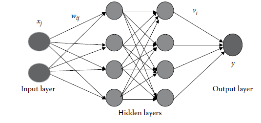 Figure 1
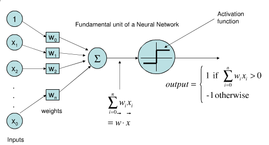 Figure 2
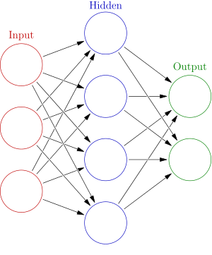 Figure 3
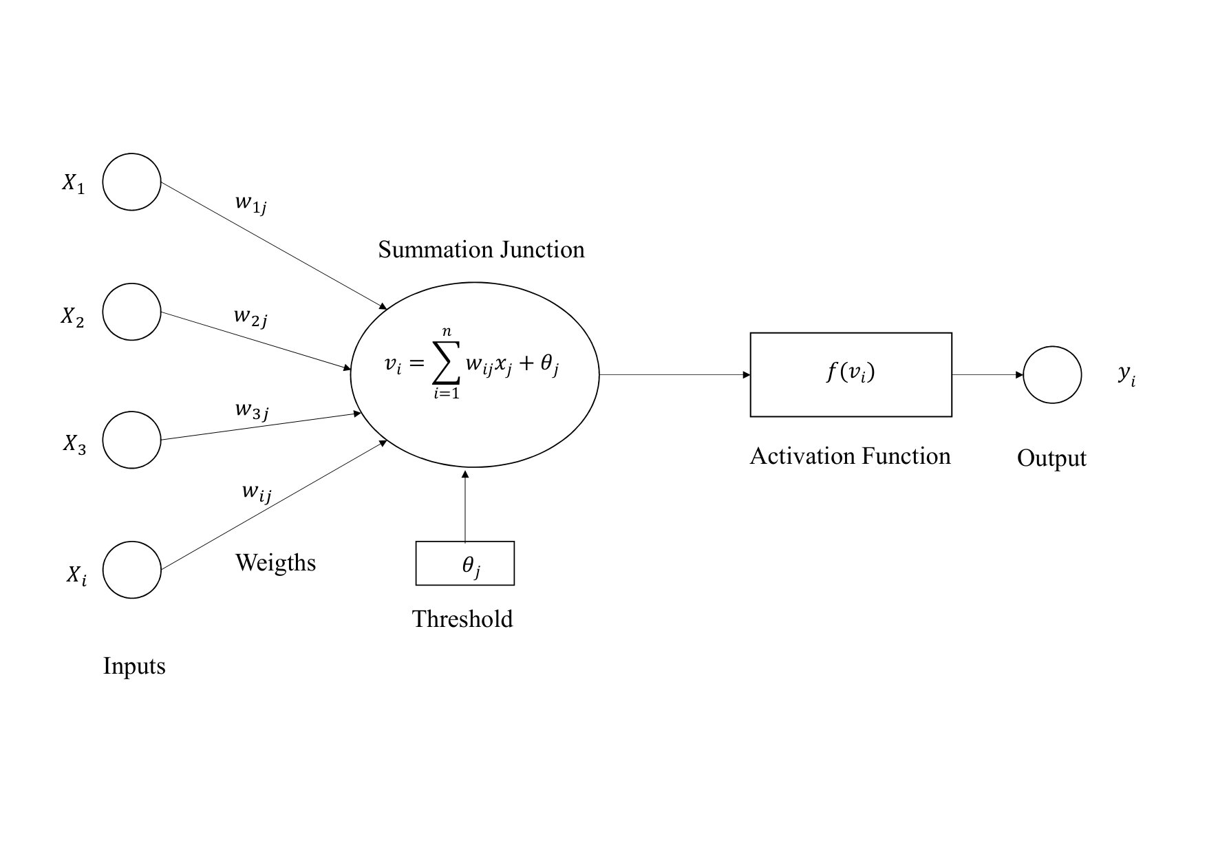 Figure 4
| This work | Ref. IZSMAIN | PE (%) | |
|---|---|---|---|
| 0.56 | |||
| 0.15 | |||
| 0.2 | |||
| 0.48 | |||
| 0.27 | |||
| 0.41 | |||
| 1.2 | |||
| 0.7 | |||
| 0.94 | |||
| 0.85 |
| This work | Ref. Govindarajan:2000vq | PE (%) Real | PE (%) Imaginary | ||
|---|---|---|---|---|---|
| 0.17 | 0.12 | ||||
| 0.56 | 0.16 | ||||
| 0.22 | 0.11 | ||||
| 0.09 | 0.07 | ||||
| 0.23 | 0.04 | ||||
| 0.02 | 0.01 | ||||
| 0.06 | 0.01 | ||||
| 0.01 | 0.01 | ||||
| 0.01 | 0.01 | ||||
| 0.03 | 0.02 |
| 0.01 | 0.1 | 0.5 | 0.99 | 0.9999 | |
|---|---|---|---|---|---|
| FNNM | |||||
| CFM |
Peer Reviews
No public reviews on file for this paper yet. If you reviewed it on a platform where reviews are public (OpenReview, ICLR, NeurIPS, ICML), you can paste yours below so the community can read it here.
Videos
No videos yet. Explain this paper in a talk, walkthrough, or lecture? Add one.
Quasinormal modes of dS and AdS Black Holes: Feedforward neural network method
Ali Övgün
[email protected] https://www.aovgun.com Physics Department, Eastern Mediterranean University, Famagusta, 99628 North Cyprus, via Mersin 10, Turkey.
İzzet Sakallı
Physics Department, Eastern Mediterranean University, Famagusta, 99628 North Cyprus, via Mersin 10, Turkey.
Halil Mutuk
Physics Department, Faculty of Arts and Sciences, Ondokuz Mayis University, 55139, Samsun, Turkey.
Abstract
In this paper, we show how the quasinormal modes (QNMs) arise from the perturbations of massive scalar fields propagating in the curved background by using the artificial neural networks. To this end, we architect a special algorithm for the feedforward neural network method (FNNM) to compute the QNMs complying with the certain types of boundary conditions. To test the reliability of the method, we consider two black hole spacetimes whose QNMs are well-known: pure de Sitter (dS) and five-dimensional Schwarzschild anti-de Sitter (AdS) black holes. Using the FNNM, the QNMs of are computed numerically. It is shown that the obtained QNMs via the FNNM are in good agreement with their former QNM results resulting from the other methods. Therefore, our method of finding the QNMs can be used for other curved spacetimes that obey the same boundary conditions.
Quasinormal modes; feedforward neural network; de Sitter; anti-de Sitter; black hole
pacs:
95.30.Sf, 04.70.-s, 97.60.Lf
I Introduction
QNMs are single frequency modes dominating the time evolution of perturbations of systems which are subject to damping, either by internal dissipation or by radiating away energy. Due to the damping, the frequency of a QNM must be complex, its imaginary part being inversely proportional to the typical damping time. Recall that, in general relativity, damping occurs even without friction, since energy may be radiated away towards infinity by gravitational waves IP1 ; IP2 . Thus, they could lead to the direct identification of the existence of the BH through gravitational wave observation, which might be realized in the near future. QNMs, which are believed to be characteristic sounds of perturbed black hole (BH) spacetimes have been investigated for a long time and their physical properties have been presented in various studies (see for example Schutz:1985zz ; Berti:2009kk ; Guinn:1989bn ; Konoplya:2011qq ; Iyer:1986nq ; CastelloBranco:2005hz ; CastelloBranco:2004nk ; Jing:2005dt ; Skakala:2010uk ; Sakalli:2013yha ; Sakalli:2011zz ; Sakalli:2018nug ; Ovgun:2018gwt ; Gonzalez:2017zdz ; Jusufi:2017trn ; Ovgun:2017dvs ; Crisostomo:2004hj ; Lepe:2004kv ; Saavedra:2005ug ; Becar:2007hu ; Becar:2010zz ; Abdalla ; Casals:2012tb ; Konoplya:2005hr ; Kuang:2017sqa ; Jusufi:2015mii ). It is worth noting that similar to the BH geometries, QNMs can also arise from other spacetimes including the wormholes Konoplya:2005et ; Kim:2008zzj ; Konoplya:2016hmd ; Oliveira:2018oha ; Sakalli:2015taa ; Sakalli:2015mka ; Ovgun:2015sqa ; Ovgun:2016ijz ; Jusufi:2017vta ; Halilsoy:2013iza ; Jusufi:2017mav ; Richarte:2017iit ; Ovgun:2018fnk ; Konoplya:2018ala ; Kim:2018ang ; Bronnikov:2012ch ; Aneesh:2018hlp ; Konoplya:2010kv ; Bueno:2017hyj ; Volkel:2018hwb ; Aragon:2020xtm ; Yan:2020hga ; Fontana:2020syy ; Panotopoulos:2020mii ; Mourier:2020mwa ; Fabris:2020kog ; Villani:2020bfc ; Chen:2020evr ; Burikham:2020dfi ; Matyjasek:2020bzc ; Aragon:2020tvq ; Awad:2017sau ; Hanafy:2015yya ; Nashed:2004pn .
Since the discovery of the AdS/CFT correspondence IZS1 , QNMs of AdS spacetimes has become very attractive over the past two decades. Besides, it is suggested that QNMs of AdS BHs are related with the double conformal field theory (CFT) IZS4 ; IZS5 ; IZS6 ; IZS7 ; IZS8 ; IZS9 . Since the QNMs govern the deterioration time of a perturbed BH, within the bulk, configuration, they should be associated with the AdS/CFT duality in order to return the boundary of Yang-Mills theory to the thermal equilibrium. The numerical computations of QNMs for AdS BHs in arbitrary dimensions were served in IZS4 . Then, Govindarajan and Suneeta IZS10 computed the QNMs of the AdS-Schwarzschild BH by using the superpotential approach. Moreover, in the framework of scalar perturbation spectra, it was known that there exists a relation between (bulk) dS spacetime and the corresponding CFT at the boundaries (past and future ) IZS11 , which provides a quantitative support for the dS/CFT correspondence. The relation between the QNMs and surface gravity () of the cosmological horizon was thoroughly discussed in IZS12 . Unlike the massless minimally coupled scalar field, it was shown that for a massive scalar field there exists QNMs in the pure dS spacetimes. Even, the obtained QNMs of pure dS spaces are analytical frequencies IZSMAIN .
New derivations of the QNMs for the curved spacetimes have always attracted a great attention. This challenge stems from the fact that it is difficult to solve the wave equations of the considered fields, analytically. Therefore, many numerical techniques have been developed in order to solve those type of equations. In recent decades, the artificial neural networks (ANNs) ann2019 are employed for finding solutions of differential equations which appeared in the different physical systems. As is well known, FNNM was the first and simplest type of ANN devised. In this network, the information moves in only one direction forward from the input nodes, through the hidden nodes (if any) and to the output nodes. There are no cycles or loops in the network FNNM . FNNM or such connectionist systems compute the systems uncertainly inspired by the biological nervous (neural) systems that constitute animal brains and also there are many applications in general relativity and cosmology Menendez-Vazquez:2020khz ; Dreissigacker:2020xfr ; Wang:2020dbt ; Vajente:2019ycy ; Ciuca:2018tei ; Khan:2020fso ; Green:2020dnx ; Santos:2020gis ; Haegel:2019uop ; Dreissigacker:2019edy ; George:2017pmj ; Gabbard:2017lja . Some of the advantages of using FNNM in solving the differential equations are listed below (Parisi:2003, ; Yadav:2015, ; Mutuk:2018erw, ; Mutuk:2019uez, ):
- •
Solution in the domain/field of integration is continuous Nakano:2018vay ,
- •
Computing complexity does not increase significantly with increasing number of sampling points and dimensions,
- •
Rounding-off error propagation does not alter the ANN solution, which happens in standard numerical methods
In this paper, we separately compute the QNMs for the four-dimensional pure dS space dSiz1 ; IZSMAIN and the AdS-Schwarzschild BH Govindarajan:2000vq by using the FNNM within the framework of supervised learning (see for instance SLearning and references therein). In fact, the supervised learning algorithm analyzes some training (educational) data and generates an inference (or the so-called trial) function that can be used to achieve new results. This requires that the learning algorithm should be reasonably generalized from the educational data to situations that are not visible. It was also shown in accuracy that the accuracy of the results obtained from the neural network surpasses the accuracy of other machine learning algorithms like SVM (support vector machines) and RF (random forest). While performing the computations, we consider the massive scalar field perturbations of the associated spacetimes. Finally, we compare the QNM values obtained with the FNNM with the results found from the other methods.
This paper is organized as follows: In Sec. II, we briefly review the QNMs of the pure dS and the AdS-Schwarzschild BH. In Sec. III, we describe the FNNM and show how one can compute the QNMs of those dS/AdS spacetimes. Then, we present and compare our results with the known ones. Finally, we conclude the paper with discussions in Sec. IV. We use natural units with .
II QNMs of Pure dS and AdS-Schwarzschild BHs
In this section, we shall make a brief overview of the QNMs of the pure dS and AdS spacetimes, which were obtained by the methods of analytical and super potential approach, respectively. We first consider the pure dS spacetime, which is given by the following line-element dSiz1 :
[TABLE]
where in which denotes the minimal radius of dS space. Furthermore, is the metric on the sphere of radius . For the massive scalar field perturbations, one should consider the Klein-Gordon equation:
[TABLE]
which can be separated by
[TABLE]
Here, is nothing but the spherical harmonics, which corresponds to the eigenfunction of two-dimensional Laplace-Beltrami operator having the eigenvalue . Recalling definition of the tortoise coordinate, we get
[TABLE]
Thus, one obtains the radial equation in the form of Schrödinger-like wave equation
[TABLE]
where the effective potential reads
[TABLE]
Since , the effective potential (6) diverges () at the singularity () and vanishes at the cosmological horizon (). For this reason, QNMs obey the following boundary conditions: purely outgoing wave at the cosmological horizon and vanish at the singularity IZSMAIN . Meanwhile, at this stage, it is worth noting the late-time tails Burko:2007ju cannot be addressed by merely studying Eq. (5) (the reader can refer to Destounis:2020pjk ). After deriving the exact analytical solution of the radial equation in terms of the hypergeometric function and in the sequel imposing the boundary conditions, it was found that to have non-zero QNMs there is a lowest bound: on the mass of scalar field . The resulting QNM sets were given by IZSMAIN as follows:
[TABLE]
The difference in sets is due to the poles of the gamma functions that help us to sort out the waves on the horizon only as outgoing waves. Without loss of generality, when comparing the above results with the FNN method to be applied, we will consider the first set as
[TABLE]
On the other hand, AdS-Schwarzschild BH is given by Govindarajan:2000vq
[TABLE]
where
[TABLE]
The relationship between and the BH mass is given by
[TABLE]
where denotes the area of a unit -sphere described by . Using the ansatz for the scalar field
[TABLE]
the massless Klein-Gordon equation of metric (10) yields the following one-dimensional Schrödinger-like wave equation:
[TABLE]
where and the effective potential becomes (for simplicity, the authors of Govindarajan:2000vq had taken and we will also stick to their choice in our computations in order to make a consistent comparison):
[TABLE]
It is clear from Eq. (15) that at spatial infinity () and vanishes at the horizon . For this reason, QNMs of obey the following boundary condition: purely ingoing wave at the horizon and vanish at the spatial infinity. Since the fundamental QNMs of the Schwarzschild BH are closely approximated by the QNMs of the Pöschl-Teller potential, in the spirit of the Pöschl-Teller method for asymptotically flat BHs, the QNMs for the AdS-Schwarzschild BH in , using a superpotential approach, was obtained and served in Table I of Govindarajan:2000vq . In general, for the asymptotically flat BHs, the QNMs correspond to solutions of the wave equations with the physical boundary conditions of purely outgoing waves at spatial infinity and purely ingoing waves crossing the event horizon myQNM1 ; myQNM2 . However, for the AdS-Schwarzschild BH, QNMs should admit wave functions that must be purely ingoing wave at the horizon and no outgoing wave at spatial infinity. Namely, at the asymptotic regions, all QNMs of the AdS BH are required to terminate. Thus, as being highlighted in Govindarajan:2000vq , any numerical calculation of QNMs is very artful due to the nature of the boundary conditions.During the numerical computations, one must ensure to have pure ingoing wave near the horizon, which could be contaminated by an outgoing wave and the correct asymptotic behavior of the wave function that fades away as . In the superpotential method Govindarajan:2000vq , as in the continued fraction method CFMiz which is suitable for the asymptotically flat BHs, a particular ansatz for the wave function was introduced to meet all boundary conditions. Similarly, in the FNNM method, a trial solution or ansatz that meets the boundary requirements will have to be sought.
III FNNM
A complicated problem in science can be solved analytically or numerically in terms of known methods. In most of the cases, an analytical solution to the associated differential equation may not be obtained easily and it is usually cumbersome. Various types of numerical methods have been developed to solve such transcendental differential equations such as shooting, Euler, Runge-Kutta, finite difference, finite element, finite volume, Adomian decomposition, asymptotic iteration, variational iteration, and perturbation methods. All these methods have both advantages and shortcomings. Although they provide good approximate solutions, these methods require discretization of the domain of the problem. Most of these numerical methods give solutions over discrete points and the solution between these points needs to be interpolated. Besides, these methods are in general iterative such that one should fix the step-size before solving the considered problem. The advantages of employing the ANNs (and whence the FNNM) can be listed as follows (Yadav:2015, ; Parisi:2003, ) :
- •
Solving differential equation by neural network framework presents solution with a very good generalization properties.
- •
The method is general and can be applied to the systems defined on either orthogonal box boundaries or on irregular arbitrary shaped boundaries.
- •
The ANN method can be implemented on parallel architectures which can be used in more complex problems.
- •
The ANN method spends negligible computing time and memory.
- •
If the model has free parameters, they can be treated as variables in the ANN method.
Most of the problems which can not be solved analytically are turned into an mathematical optimization problem in which a numerical solution is sought. This optimization can be done in some techniques. Since the problem is considered in a specific region (i.e., the convergence problem), the transition between local and global solutions require intensive processing. In this perspective, the ANNs have broad usage field and they are powerful tools for performing a mathematical modeling.
An ANN can be defined as parallel information processor in which a number of neurons are distributed as operating units. This information processing systems can take many input from outside, combines them via mostly nonlinear operations and produce the output. Nowadays, ANN is one of the popular topics of machine learning paradigm. They have a wide range of usage from pattern recognition to financial forecast including classification, decoding speech etc. ANNs are typically composed of layers. These layers are made of interconnected neurons (perceptrons in modern computers). A neuron is the main processing element in the ANN. Because, neurons have activation functions which translate input signals to output signals. Problem solving process in the ANN occurs by acquiring knowledge. This mechanism is maintained by learning methods and information is stored within ’inter-neuron connections’ strength which can be calculated by some numerical values called weights Chak ; mtk .
The detailed computational steps of the working principle of an artificial neuron in a neural network can be seen in in Fig. (1).
A neuron receives inputs which belong to . Each input is multiplied by a weight factor for before entering to the neuron . In general, this neuron has a bias term and a critical value . To produce the output signal, this critical value must be reached and / or exceeded. The input of the -th neuron in the input layer can be written as
[TABLE]
The neurons in the input layer can work only if the signal reaches/exceeds the critical value which can be defined as the neuron’s working condition as
[TABLE]
All the input signals are multiplied by their synaptic weights and added together. This compose ”‘net”’ input to the neuron:
[TABLE]
where is the threshold (i.e., critical) value. The output signal of -th neuron the can be functionalized as
[TABLE]
An activation function acts on the produced weighted signal which is denoted as . The output signal can be obtained by mapping this activation function as
[TABLE]
where denotes the neuron activation function. This output function is suggested together with a critical function. In this present work, we will use a sigmoid activation function
[TABLE]
which is a traditional one for obtaining solutions in nonlinear problems.
A diagram of a multilayer ANN is given in Fig. (2).
The information are given to the input layer, which sends the information to the hidden layer, if any exists. The processing of inputs are being done at this stage via a system of weighted connections. The hidden layers send the information to the output layer and an answer is given to the outside world. In Fig. (2), are input nodes, are weights from input to the hidden layer (or layers if exist), and are synaptic weights from hidden to the output layer which is the output node Chak . The neurons in the same layer have no connection among themselves.If there is more than one hidden layer, the architecture is known as deep neural network which is out of the scope of the present work.
In the present work we have used an architecture which consists of one input layer, one hidden layer and one output layer. This ANN architecture can be seen in Fig. 3. Neurons are arranged into distinct layers with each layer receiving input from the previous layer and outputting to the next layer. In this manner, neurons (processing elements) in a layer receive input from the previous layer and send (feed) their output to the next layer.
Initial weights from the input layer to the hidden layer () and from the hidden layer to the output layer () are taken as arbitrary (random). The number of nodes in the hidden layer are determined by the trial-and-error method.
III.1 Implementation of ANN on Quantum Systems
The framework for FNNM to obtain solutions of eigenvalue equations was developed in Ref. Lagaris:1997ap . A differential equation can be written as
[TABLE]
with
[TABLE]
Here, is a linear operator, is a known function and is the boundary of . In order to solve Eq. (22), a trial function
[TABLE]
can be used. This function proceeds to a neural network with a vector parameter and undetermined parameter which is going to be adjusted later. is a single-output feed forward neural network with parameters and input units fed with the input vector . The functions and will be determined with respect to appropriate which satisfies the boundary conditions.
To solve Eq. (22), the collocation method collo can be used. The idea behind the collocation method is to choose a finite-dimensional space of trial solution functions and a number of points in the domain of the problem, and to select that trial solution which satisfies the given equation at the collocation points. This procedure discrete the domain into a set of . To this end, one can get a minimization problem as follows:
[TABLE]
To have the Schrödinger equation, one can recast Eq. (22) in an eigenvalue equation:
[TABLE]
with the boundary condition . Before obtaining QNMS via FFNM, an important notice should be done. In this work, we assume the foreknown definition of the QNMs that these modes are purely outgoing waves at the event horizon of black hole , where is the boundary defining the region of space around a black hole from which nothing (not even light) can escape and vanish at IZSMAIN . These boundary conditions are determined by the behavior of the effective potential: recall Eqs. (6) and (15), which are obtained for dS and AdS spacetimes, respectively. Thus, the trial solution becomes
[TABLE]
where at boundaries for a range of values. Employing the discretization for the domain of the problem together with the collocation method, a minimization problem can be obtained with respect to the and :
[TABLE]
where represents the error function. Furthermore, is obtained as follows
[TABLE]
Thus, the energy eigenvalues or the QNMs are given by
[TABLE]
where represents the location where the scalar field becomes pure plane wave (ingoing/outgoing) and indicates the radial position where the effective potential diverges and whence causes the waves to be completely damped (i.e., ). Therefore, while and for the pure dS BH, in the AdS BH we take and corresponds to the effective potential of the spacetime taken into account.
The parameter is nothing but the weights and biases of the ANN. Although the multi-layer sensor (MLP) has many hidden layers, here we use a simple model of a single hidden layer MLPs. In this study, we also consider a multilayer perception with input units, one hidden layer having units, and an output. Given an input vector
[TABLE]
the output of the neural network can be written as
[TABLE]
where
[TABLE]
Here, are the weights from input unit to the hidden unit , is the weight from hidden unit to the output unit, represents the bias of hidden unit , and is the sigmoid function, which is given in Eq. (21). The derivatives of the ANN output can be written as
[TABLE]
where and is the order derivative of the activation (sigmoid) function.
One can parametrize the solution trial function as
[TABLE]
where denotes a feedforward neural network with one hidden layer and sigmoid hidden units
[TABLE]
The minimization problem turns out to be as
[TABLE]
Solving this equation is equivalence to solving Schrödinger equation. The minimization problem can be solved via collocation method. In this method, one chooses a finite dimensional space of solution trial function which is supposed to solve given differential equation with a number of points in the domain.
In order to obtain desired result, ANN needs to learn. Solving a differential equation within ANN method requires training of the ANN. This learning process can be done in different ways. In this work, we used error back-propagation learning algorithm. This learning algorithm is one of the most common used learning rules and it is valid for continuous activation function such as sigmoid function Eq. (21). By taking the partial derivative of the error function according to each weight, we can monitor the flow of the error direction in the network. The steps for the learning algorithm of back-propagation is as follows Chak ; mtk :
- 1
Set the weights and from the hidden to the output layer. Choose the learning parameter in the range , and error . At the first step, error is taken to be zero. 2. 2
Train the network. 3. 3
Find the output of error function. 4. 4
Calculate the error signal terms by output and hidden layers, respectively. 5. 5
Calculate the error components for gradient vectors. 6. 6
Check if weights are adjusted appropriately. 7. 7
If , then cease the training. If not, proceed to step 2 by setting and initiate the new training.
The crucial point for the training process is taking the eigenvalue (error function) as zero and train the neural network with equidistant points in the given interval of the problem. It is expected that this process yields energy function (eigenvalue) to be zero or at least converge to zero. If the convergence is not obtained, then the eigenvalue is wrong. If this happens, eigenvalue should be changed in a proper way and the training process should be restarted. It should be keep doing this process until the energy (error) function converges to zero.
It should also be noted that the method for solving differential equations with ANNs does not depend on the training method: The choice of training method only effects the speed of the training procedure.
III.2 QNMs of Pure dS and AdS-Schwarzschild BHs via FNNM
To derive the QNMS of the pure dS and AdS-Schwarzschild BHs, we first consider Eqs. (6) and (15), respectively, in Eq. (30), then compute the QNMs with the expression seen in Eq. (30). To this end, we employ the Gauss-Legendre rule Lagaris:1997ap and use 200 equidistant points in the interval with . In Tables I and II, we represent our findings, which are the numerical values (via the FNNM within the context of supervised learning) of the QNMs of the pure dS and AdS spacetimes. It can be seen from those Tables that FNNM satisfactorily re-derives the well-accepted QNMs’ results obtained from the other methods IZSMAIN ; Govindarajan:2000vq . Thus, we have managed to introduce a new and effective method to the literature for computing the QNMs.
As mentioned above, the main advantage of using ANN is to solve the Schrödinger equation. However, the computational complexity while using the ANN does not increse considerably with the number of sampling points and with the number of dimensions in the problem. Depending on the learning algorithm, the running CPU time can be lowered significantly to obtain the solution. On the other hand, we shall not perform any CPU time comparison in this study, because it is irrelevant with the scope of the paper.
IV Conclusions
In this study, we have prescribed a new method, FNNM, to study the QNMs of BHs that posses particular boundary conditions as being described in Sec. II. To test the method, we have considered the pure dS and AdS-Schwarzschild BHs. Scalar field perturbations have been treated as oscillations in the frequency domain of those static and symmetric backgrounds. In each geometry, the perturbed scalar fields are reduced to Schrödinger like wave equations with the associated effective potential. Imposing the required boundary conditions given in Refs. IZSMAIN and Govindarajan:2000vq , we have demonstrated how the FNNM derives the QNMs: the resulting formula is Eq. (30). After comparing our findings with the previous results obtained by the analytical method IZSMAIN and the superpotential approach (numerical) method Govindarajan:2000vq , it is seen that the all results are in good agreement with each other. Therefore, FNNM is not only an alternative but an effective way for computing the QNMs that are important for the stability of a BH and the late-time behavior of radiation from gravitationally collapsing configurations. On the other hand, one may ask that how about for neural network solutions to the completely unknown problems. For such a case the architecture and training processes must be different than the FNNM that we employed here. In fact, such an architecture is more about interacting with “experimental data” like “a* direct adaptive neural network method*“ example in which the system took into account was described by an unknown NARMA model NARMA and the FNNM was considered to learn the system. By taking the FNNM as a neural model, the control signals can easily be obtained by minimizing momentary difference or cumulative differences between a set point and the output of the FNNM. Since the training algorithm can ensure that the output of the FNNM approaches to the real system, then it can be demonstrated how the obtained control signals make the real system output as being close to the set point example2 . However, such an algorithm cannot be established without having experimental data on the BHs that we work with. Namely, with the development of technology related to the BHs, it might be possible to construct such a neural network algorithm.
Further work to determine the QNMs of rotating and/or higher/lower dimensional dS/AdS spacetimes via the FNNM could therefore be interesting. Besides, we aim to extend our analysis to the Dirac (e.g., the reader is referred to this recent study fermion ) and Maxwell equations that are formulated in the Newman-Penrose formalism mynp1 ; mynp2 ; mynp3 in the near future. Moreover, starting from Kerr BH, we also plan to analyze the QNMs myq1 ; myq2 ; myq3 ; myq4 ; myq5 of various stationary spacetimes.
Acknowledgements.
We are thankful to the Editor and anonymous Referees for their constructive suggestions and comments. APPENDIX Metric of the Reissner-Nordström BH of mass and charge is given by
[TABLE]
where . The locations of the event horizon and of the Cauchy horizon are and , respectively. To investigate the bosonic perturbation of the Reissner-Nordström BH, one should consider the scalar field , which obeys the Klein-Gordon equation (2), propagating in a Reissner-Nordström BH geometry. For the chargeless case with an Ansatz , the radial components of the fields can be found as follows izs1 :
[TABLE]
where and is a separation constant. If one makes the following transformation and adopt the tortoise coordinate (defined here as , the radial equation (A2) recasts in
[TABLE]
where the complex function is given by
[TABLE]
By comparing Eqs. (14) and (A3), one can easily derive the effective potential of the Reissner-Nordström BH:
[TABLE]
Following the Leaver’s izs2 ; izs3 original continued fraction method (CFM), which was later improved by Nollert izs4 , with the effective potential (A5), Richartz and Giugno izs5 obtained the numerical values of the QNMs of the Reissner-Nordström BH. Comparing the numerical results of Ref. izs5 with the results to be obtained from FNNM might be more meaningful and beneficial for the reader. For this purpose, we have created Table III, which obviously shows how the two methods produce very close values.
The reference list from the paper itself. Each links out to its DOI / PubMed record.
- 1(1) L. Manfredi, J. Mureika, and J. Moffat, ”Quasinormal Modes of Modified Gravity (MOG) Black Holes,” JURP, 29 , 100006 (2019).
- 2(2) P. D. Roy, S. Aneesh, and S. Kar, ”Revisiting a family of wormholes: geometry, matter, scalar quasinormal modes and echoes”, The European Physical Journal C 80 , 850 (2020).
- 3(3) B. F. Schutz and C. M. Will, “Black Hole Normal Modes: A Semianalytic Approach,” Astrophys. J. 291 , L 33 (1985).
- 4(4) E. Berti, V. Cardoso and A. O. Starinets, “Quasinormal modes of black holes and black branes,” Class. Quant. Grav. 26 , 163001 (2009).
- 5(5) J. W. Guinn, C. M. Will, Y. Kojima and B. F. Schutz, “High Overtone Normal Modes of Schwarzschild Black Holes,” Class. Quant. Grav. 7 , L 47 (1990).
- 6(6) R. A. Konoplya and A. Zhidenko, “Quasinormal modes of black holes: From astrophysics to string theory,” Rev. Mod. Phys. 83 , 793 (2011)
- 7(7) S. Iyer, “Black Hole Normal Modes: A Wkb Approach. 2. Schwarzschild Black Holes,” Phys. Rev. D 35 , 3632 (1987).
- 8(8) K. H. C. Castello-Branco, R. A. Konoplya and A. Zhidenko, “High overtones of Dirac perturbations of a Schwarzschild black hole and the area spectrum of quantum black holes,” Braz. J. Phys. 35 , 1149 (2005).