Criteria for the a-contraction and stability for the piecewise-smooth solutions to hyperbolic balance laws
Sam G. Krupa (The University of Texas at Austin)

TL;DR
This paper proves the uniqueness and stability of piecewise-smooth solutions with extremal shocks for hyperbolic balance laws, applicable to gas dynamics, without smallness assumptions and under mild conditions.
Contribution
It extends the theory of a-contraction to hyperbolic balance laws with shocks of any size, ensuring stability and uniqueness under minimal hypotheses.
Findings
Proves $L^2$ stability for solutions with extremal shocks.
Handles shocks of arbitrary size without smallness assumptions.
Works under mild hypotheses, including a weak trace condition.
Abstract
We show uniqueness and stability in and for all time for piecewise-smooth solutions to hyperbolic balance laws. We have in mind applications to gas dynamics, the isentropic Euler system and the full Euler system for a polytropic gas in particular. We assume the discontinuity in the piecewise smooth solution is an extremal shock. We use only mild hypotheses on the system. Our techniques and result hold without smallness assumptions on the solutions. We can handle shocks of any size. We work in the class of bounded, measurable solutions satisfying a single entropy condition. We also assume a strong trace condition on the solutions, but this is weaker than . We use the theory of a-contraction (see Kang and Vasseur [Arch. Ration. Mech. Anal., 222(1):343--391, 2016]) developed for the stability of pure shocks in the case without source.
Click any figure to enlarge with its caption.
 Figure 1
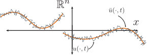 Figure 2
Peer Reviews
No public reviews on file for this paper yet. If you reviewed it on a platform where reviews are public (OpenReview, ICLR, NeurIPS, ICML), you can paste yours below so the community can read it here.
Videos
No videos yet. Explain this paper in a talk, walkthrough, or lecture? Add one.
Criteria for the a-contraction and stability for the piecewise-smooth solutions to hyperbolic balance laws
Sam G. Krupa
Department of Mathematics
The University of Texas at Austin
Austin, TX 78712
USA
(Date: April 20th, 2019)
Abstract.
We show uniqueness and stability in and for all time for piecewise-smooth solutions to hyperbolic balance laws. We have in mind applications to gas dynamics, the isentropic Euler system and the full Euler system for a polytropic gas in particular. We assume the discontinuity in the piecewise smooth solution is an extremal shock. We use only mild hypotheses on the system. Our techniques and result hold without smallness assumptions on the solutions. We can handle shocks of any size. We work in the class of bounded, measurable solutions satisfying a single entropy condition. We also assume a strong trace condition on the solutions, but this is weaker than . We use the theory of a-contraction (see Kang and Vasseur [Arch. Ration. Mech. Anal., 222(1):343–391, 2016]) developed for the stability of pure shocks in the case without source.
Key words and phrases:
System of conservation laws, compressible Euler equation, Euler system, isentropic solutions, generalized Riemann problem, piecewise-smooth solutions, Rankine–Hugoniot discontinuity, shock, stability, uniqueness.
2010 Mathematics Subject Classification:
Primary 35L65; Secondary 76N15, 35L45, 35A02, 35B35, 35D30, 35L67, 35Q31, 76L05, 35Q35, 76N10
This work was partially supported by NSF Grant DMS-1614918.
Contents
1. Introduction
We consider an system of balance laws,
[TABLE]
For a fixed (including possibly ), the unknown is . The function is in and is the initial data. The function is the flux function for the system. The source term is translation invariant. We also ask that be Lipschitz continuous from for every interval , with a Lipschitz constant uniform in . In other words, there exists such that
[TABLE]
for every and for every interval . Furthermore, we require that is bounded on :
[TABLE]
for every .
We assume the system (1.1) is endowed with a strictly convex entropy and associated entropy flux . Note the system will be hyperbolic on the state space where exists. We assume the functions , and are defined on an open convex state space . We assume and . By assumption, the entropy and its associated entropy flux verify the following compatibility relation:
[TABLE]
By convention, the relation (1.4) is rewritten as
[TABLE]
where denotes the matrix .
For where exists , the system (1.1) is hyperbolic, and the matrix is diagonalizable, with eigenvalues
[TABLE]
called characteristic speeds.
We consider both bounded classical and bounded weak solutions to (1.1). A weak solution is bounded and measurable and satisfies (1.1) in the sense of distributions. I.e., for every Lipschitz continuous test function with compact support,
[TABLE]
We only consider solutions which are entropic for the entropy . That is, they satisfy the following entropy condition:
[TABLE]
in the sense of distributions. I.e., for all positive, Lipschitz continuous test functions with compact support:
[TABLE]
For , the function defined by
[TABLE]
is a weak solution to (1.1) if and only if , and satisfy the Rankine-Hugoniot jump compatibility relation:
[TABLE]
in which case (1.10) is called a shock solution.
Moreover, the solution (1.10) will be entropic for (according to (1.9)) if and only if,
[TABLE]
In this case, is an entropic Rankine–Hugoniot discontinuity.
For a fixed , we consider the set of which satisfy (1.11) and (1.12) for some . For a general strictly hyperbolic system of conservation laws endowed with a strictly convex entropy , we know that locally this set of values is made up of curves (see for example [32, p. 140-6]).
The present paper concerns the finite-time stability of piecewise-smooth solutions to (1.1), working in the setting. We work in a very general setting. Our techniques are based on the theory of shifts as developed by Vasseur within the context of the relative entropy method (see [45]). We consider systems of the form (1.1), with minimal assumptions on the shock families. We ask that the extremal shock speeds (1-shock and n-shock speeds) are separated from the intermediate shock families. If we want to consider 1-shocks, we ask that the 1-shock family satisfy the Liu entropy condition (shock speed decreases as the right-hand state travels down the 1-shock curve), and we ask that the shock strength increase in the sense of relative entropy (an requirement) as the right-hand state travels down the 1-shock curve. If we want to consider n-shocks, we ask for similar requirements on the n-shock family.
The intermediate wave families have far fewer requirements. The intermediate shock curves might not even be well-defined and characteristic speeds might cross.
In particular, the results in this article apply to both the isentropic Euler system and the full Euler system for a polytropic gas, viewing both systems in Eulerian coordinates.
We study solutions which are piecewise-Lipschitz continuous in the space variable . We study the stability and uniqueness of these solutions among a large class of weak solutions which are bounded, measurable, entropic for at least one strictly convex entropy, and verify a strong trace condition (weaker than ). We do not make small data assumptions. We require the piecewise-smooth contain a single shock of extremal family. However, the rougher solutions which we compare to this solution may have shocks of any type or family.
Previous results in the theory of stability and a-contraction have only been able to consider initial data which is pure shock (piecewise constant). This present paper extends the ideas in the theory of a-contraction (in particular as developed in [26]).
The point of the present article is this: As discussed for the case of nonlocal scalar balance laws in [30], when studying the stability up to a translation in space of solutions piecewise-constant in space, we can view the shift function which is doing the translation as simply determining at which points do we want to see the left hand state of our solution, and at which points do we want to see the right hand state of our solution. However, for piecewise-smooth data, the shift function cannot be viewed like this. Instead, the shift function is viewed as artificially translating in space our solution. If the solution is non-constant away from the discontinuity, this artificial translation creates a linear term in the entropy dissipation (see Lemma 3.3), which we cannot Gronwall in comparison with the quadratic terms. The answer is to create a shift function which not only neutralizes entropy production at the discontinuity of the solution, but also creates additional negative entropy (see Proposition 4.1) we can use to cancel out the linear term in the Gronwall argument (see Figure 1). Regarding the idea of additional negative entropy caused by a shift, see [25].
This work is related to the generalized Riemann problem, which concerns solutions with initial data which is piecewise-smooth instead of simply piecewise-constant across a single jump discontinuity. For existence and uniqueness results for the generalized Riemann problem, see [36, 35]. However, these results have small data limitations.
Previous results in this direction include Chen, Frid, and Li [9] where for the full Euler system, they show uniqueness and long-time stability for perturbations of Riemann initial data among a large class of entropy solutions (locally and without smallness conditions) for the Euler system in Lagrangian coordinates. They also show uniqueness for solutions piecewise-Lipschitz in . For an extension to the relativistic Euler equations, see Chen and Li [10]. However, these papers do not give stability results for all time.
We study the stability in of piecewise-smooth solutions to the system of balance laws (1.1). The study of piecewise-smooth solutions takes us a step beyond the classical Riemann problem, which considers piecewise-constant initial data. Furthermore, when the system (1.1) has the source term , it is important to study piecewise-smooth solutions and just not piecewise-constant, for the source term may mean that even pure shock wave initial data evolves into something more complicated. For a nonlocal example of this phenomenon, consider the solution to the Riemann problems for the Burgers–Hilbert equation, which is Burgers equation with a nonlocal source term [7, 8, 24, 23].
Our method is the relative entropy method, a technique created by Dafermos [15, 14] and DiPerna [21] to give -type stability estimates between a Lipschitz continuous solution and a rougher solution, which is only weak and entropic for a strictly convex entropy (the so-called weak-strong stability theory). For a system (1.1) endowed with an entropy , the technique of relative entropy considers the quantity called the relative entropy, defined as
[TABLE]
Similarly, we define relative entropy-flux,
[TABLE]
Remark that for any constant , the map is an entropy for the system (1.1), with associated entropy flux . Furthermore, if is a weak solution to (1.1) and entropic for , then will also be entropic for . This can be calculated directly from (1.1) and (1.8) – note that the map is basically plus a linear term.
Moreover, by virtue of being strictly convex, the relative entropy is comparable to the distance, in the following sense:
Lemma 1.1**.**
For any fixed compact set , there exists such that for all ,
[TABLE]
The constants depend on and bounds on the second derivative of .
This lemma follows from Taylor’s theorem; for a proof see [34, 45].
Given a Lipschitz solution to (1.1), and a weak, entropic solution , the method of relative entropy gives estimates on the growth in time of the quantity
[TABLE]
by studying the time derivative and using the entropy inequality (1.8). By (1.1), we get -type stability estimates.
Introducing a discontinuity into causes difficulties in the method of relative entropy. In particular, simple examples for the scalar conservation laws show that a discontinuity in prevents stability between and in the form of the classical weak-strong estimates.
However, by allowing the discontinuity in to move with an artificial speed which depends on , we can recover weak-strong type estimates. Within the context of the relative entropy method, this theory of stability up to a shift was initiated in [45] by Vasseur. Over the last decade, this theory of stability up to a shift has been matured and developed by Vasseur and his team. The first result was for pure shock wave initial data for the scalar conservation laws [33]. Further results include work on the scalar viscous conservation laws in both one space dimension [27] and multiple [28]. Recently, work on the scalar conservation laws has allowed for many discontinuities to exist in the otherwise smooth – with each discontinuity shifted in such a way as to maintain stability between and an arbitrary weak solution entropic for at least one entropy. With this, it is possible to make comparisons between two solutions which satisfy only one entropy condition, and thus show that one entropy condition is enough for uniqueness. See [29] (and the references therein) for more details. To study the stability of pure shock wave initial data in the systems case, the technique of a-contraction was introduced [26, 44, 46, 42, 34]. For a general overview of theory of shifts and the relative entropy method, see [43, Section 3-5]. By considering stability up to a shift, the method of relative entropy can also be used to study the asymptotic limit when the limit is discontinuous (see [13] for the scalar case, [47] for systems). There is a long history of using the relative entropy method to study the asymptotic limit. However, without the theory of shifts, it appears that only limits which are Lipschitz continuous can be studied (see [37, 40, 4, 1, 48, 2, 5, 22] and [45] for a survey).
The present article is a further step in the program of stability up to a shift.
In this paper, we continue the ideas introduced in [30]. In [30], it is shown that the generalized characteristics of can be used as shift functions to kill growth in between a piecewise smooth solution and weak solution to (1.1) entropic for the entropy . Further, using the generalized characteristic as a shift function provides various benefits over using the previous shift function constructions, as discussed in [30].
In this paper, we bring novel ideas from the scalar case in [30] to the systems case. In the systems case, we need to use the theory of a-contraction.
For the case of scalar, the generalized characteristics for are the natural shift functions to be using. In the systems case, we use a shift function which again is based on the generalized characteristics, but with a correction where the shift travels at greater-than-characteristic-speed due to a-contraction and the existence of multiple shock families in the systems case.
On top of the benefits for generalized-characteristic-based shifts mentioned in [30] (such as simplicity of analysis, ease of construction, enhanced control on the shifts, and strictly negative entropy creation) the use of generalized-characteristic-based shifts for the systems case allows for simplified proofs compared to the previous state-of-the-art a-contraction result, [26]. By having very obvious control on the speed of generalized-characteristic-based shifts, we are able to obviate the need for many of the computations in the foregoing analysis [26].
For systems of conservation laws in one space dimension such as (1.1) (including the scalar conservation laws), we have non-uniqueness for solutions. We impose entropy conditions such as (1.8), motivated by physics, to try to weed out “nonphysical” solutions which have physical entropy decreasing (or according to (1.8), mathematical entropy increasing). Remark that requiring more than one entropy condition (for more than one entropy) is impractical – many systems only admit a single nontrivial entropy. In the scalar case, this approach has had tremendous success. In fact, requiring solutions satisfy the entropy condition (1.8) for at least one strictly convex entropy in is enough to get uniqueness for solutions (see [41, 18, 29]). However, even for the scalar case proving uniqueness with a single entropy condition has proved difficult. The first result [41] was not until 1994. Furthermore, the first two results [41, 18] use techniques limited to the scalar case. They use the special connection between scalar conservation laws in one space dimension and Hamilton–Jacobi equations: the space derivative of the solution to a Hamilton–Jacabi equation is formally the solution to the associated scalar conservation law. Notably, [29] gives a proof of the single entropy condition for scalar conservation laws which works directly on the conservation law and utilizes the theory of shifts. Moreover, progress for uniqueness of entropic solutions to systems of conservation laws has been slow. The best theory so far is the Bressan, Crasta, and Piccoli theory [6] for uniqueness in the class of solutions with small total variation. It would be interesting however to study the uniqueness of these solutions amongst a larger class. For example, existence of solutions with large data is known for the Euler system – but the uniqueness theory for such solutions with large data lags behind.
The situation for the hyperbolic conservation laws in multiple space dimensions is even more dire – there is non-uniqueness for entropic solutions to incompressible and compressible Euler by virtue of the many highly oscillatory solutions created via convex integration or related techniques. For incompressible Euler, see two papers by De Lellis and Székelyhidi [19, 20]. For compressible Euler, see [11, 12, 39].
However, there is still the possibility of pushing forward the theory of uniqueness for hyperbolic systems of conservation laws in one space dimension. The current paper is a step in that direction – utilizing the -type relative entropy method and the constantly evolving theory of shifts.
In this article, we use the method of relative entropy, the theory of shifts and a-contraction. These theories are not perturbative. They enable us to get results without small data limitations. Further, by the nature of these theories, we only use a single entropy condition.
We present our main and most important theorem regarding -type stability and uniqueness results. The hypotheses and in the theorem depend only on the hyperbolic part of the system (1.1) and the fixed piecewise-smooth solution . The hypotheses are related to conditions on 1-shocks and n-shocks and in particular are satisfied by the isentropic Euler and full Euler systems. These hypotheses are explained in detail in Section 2.
Theorem 1.2** (Main theorem – stability for entropic piecewise-Lipschitz solutions to hyperbolic systems of balance laws).**
Fix .
Fix . Assume that . If contains a 1-shock, assume the hypotheses hold. Likewise, if contains an n-shock, assume the hypotheses hold. Assume that and are entropic for the entropy . Assume that is Lipschitz continuous on and on , where is a Lipschitz function . Assume also that verifies the strong trace property (Definition 2.1). Assume also that there exists such that for all
[TABLE]
Then there exists a Lipschitz continuous function with and constants such that,
[TABLE]
for all .
Moreover, we have control on :
[TABLE]
Remark*.*
- •
The constants depend on , , , , and bounds on the derivatives of on the range of and . In addition, depends on (see (1.2)), , , , and bounds on the derivatives of on the range of and . Note that only depends on bounds on the derivatives of and (on the range of and ).
- •
As opposed to (1.3), the proof of Theorem 1.2 will in fact go through whenever we have an estimate of the form
[TABLE]
for and some constant . Note that and (1.3) implies (1.19).
- •
Note that Hölder’s inequality and (1.18) give control on the shift in the form of
[TABLE]
- •
Note that by Property (b) of or , condition (4.1) is equivalent to the existence of a such that for all
[TABLE]
where satisfies .
The outline of the paper is as follows: in Section 2, we give our hypotheses on the system. In Section 3, we present technical lemmas. In Section 4, we construct the shift with the additional entropy dissipation. Finally, in Section 5 we prove the main theorem by using the additional entropy dissipation from the shift to translate in the piecewise-smooth solution artificially.
2. Hypotheses on the system
We will consider the following structural hypotheses , on the system (1.1),
(1.8) regarding the 1-shock and n-shock curves (they are closely related to hypotheses in [34] and [26]). For a fixed piecewise smooth solution (as in the context of the main theorem Theorem 1.2):
- •
: (Family of 1-shocks verifying the Liu condition) There exists such that for all , and for all , there is a 1-shock curve (issuing from ) (possibly ) parameterized by arc length. Moreover, and the Rankine-Hugoniot jump condition holds:
[TABLE]
where is the velocity function. The map is Lipschitz on . Further, the maps and are both on , and the following conditions are satisfied:
[TABLE]
- •
: If is an entropic Rankine-Hugoniot discontinuity with shock speed , then .
- •
: If (with , for ) is an entropic Rankine-Hugoniot discontinuity with shock speed verifying
[TABLE]
then is in the image of . In other words, there exists such that (and by implication, ).
Similarly, we will consider the following structural hypotheses on the system (1.1), (1.8) regarding the n-shock curves:
- •
: (Family of n-shocks verifying the Liu condition) There exists such that for all , and for all , there is an n-shock curve (issuing from ) (possibly ) parameterized by arc length. Moreover, and the Rankine-Hugoniot jump condition holds:
[TABLE]
where is the velocity function. The map is Lipschitz on . Further, the maps and are both on , and the following conditions are satisfied:
[TABLE]
- •
: If is an entropic Rankine-Hugoniot discontinuity with shock speed , then .
- •
: If (with , for ) is an entropic Rankine-Hugoniot discontinuity with shock speed verifying
[TABLE]
then is in the image of . In other words, there exists such that (and by implication, ).
Remark*.*
See [34, 26] for remarks on these hypotheses. We include them here for completeness. In particular,
- •
Note that the system (1.1) verifies the hypotheses - on the 1-shock family if and only if the system
[TABLE]
verifies the properties - for the n-shock family. It is in this way that - are dual to -.
- •
On top of the Liu entropy condition (Property (a) in ), we also assume Property (b), which says that the 1-shock strength grows along the 1-shock curve when measured via the pseudo-distance of the relative entropy (recall that the map measures -distance somehow – see (1.1)). This growth condition arises naturally in the study of admissibility criteria for systems of conservation laws. In particular, Property (b) ensures that Liu admissible shocks are entropic for the entropy even for moderate-to-strong shocks (see [16, 31, 38]).
In [3], Barker, Freistühler, and Zumbrun show that stability and in particular contraction fails to hold for the full Euler system if we replace Property (b) with
[TABLE]
This shows that it is better to measure shock strength using the relative entropy rather than the entropy itself.
- •
Recall the famous Lax E-condition for an i-shock ,
[TABLE]
The hypothesis is implied by the first half of the Lax E-condition along with the hyperbolicity of the system (1.1). In addition, we do not allow for right 1-contact discontinuities.
- •
The hypothesis is a statement about the well-separation of the 1-shocks from all other Rankine-Hugoniot discontinuities entropic for ; the 1-shocks do not interfere with any other shocks. In particular, will hold for any strictly hyperbolic system in the form (1.1) if all Rankine-Hugoniot discontinuities entropic for lie on an i-shock curve for some and the extended Lax admissibility condition holds:
[TABLE]
where and . Moreover, we only use the first inequality in (2.8) and the fact that for all and for all .
Furthermore, note that for any strictly hyperbolic system in the form (1.1), if and live in a fixed compact set, then there exists such that (2.8) will hold if . Similarly, for any strictly hyperbolic system endowed with a strictly convex entropy, all Rankine-Hugoniot discontinuities entropic for will locally be in the form for some , and where is the i-shock curve issuing from . See [32, Theorem 1.1, p. 140] and more generally [32, p. 140-6]. For the full Euler system , will hold regardless of the size of the shock .
- •
Fix . Then, for all with and for all , we have
[TABLE]
Note that
[TABLE]
and
[TABLE]
due to .
Recall also that by hypothesis , is parameterized by arc length. Thus, for all . We can then use (2.9) and Lemma 1.1 to get,
[TABLE]
for all with and for all . The constants depend only on and . This says that is comparable to the shock strength .
- •
On the state space where the strictly convex entropy is defined, the system (1.1) is hyperbolic. Further, by virtue of , the eigenvalues of vary continuously on the state space . Further, if the eigenvalue () is simple for (such as when the system (1.1) is strictly hyperbolic), the map () will be in due to the implicit function theorem.
We study solutions to (1.1) among the class of functions verifying a strong trace property (first introduced in [34]):
Definition 2.1**.**
Fix . Let verify . We say has the strong trace property if for every fixed Lipschitz continuous map , there exists such that
[TABLE]
for all .
Note that for example a function will satisfy the strong trace property if for each fixed , the right and left limits
[TABLE]
exist for almost every . In particular, a function will have strong traces according to Definition 2.1 if has a representative which is in . However, the strong trace property is weaker than .
3. Technical Lemmas
Throughout this paper, we use the following definition for the relative flux
[TABLE]
and the relative : for ,
[TABLE]
.
The following lemma from [46] describes how the relative entropy obeys a sort of triangle inequality:
Lemma 3.1** (Structural lemma from [46] - triangle inequality for the relative entropy).**
For any , we have
[TABLE]
and
[TABLE]
Thus, for any ,
[TABLE]
The proof of Lemma 3.1 follows immediately from the definition of and . In particular, see [26, p. 360-1] for a simple proof.
Lemma 3.2**.**
Fix . Then there exists a constant depending on such that the following holds:
If with , then whenever verify
[TABLE]
then for all .
Remark*.*
The set is compact.
The proof of Lemma 3.2 is found in the proof of Lemma 4.3 in [26]. We repeat the proof in Section 6.1 for the reader’s convenience.
The following Lemma gives the entropy dissipation caused by changing the domain of integration, translating the solution in (by a function ), and from the source term .
Lemma 3.3** (Local entropy dissipation rate).**
Fix . Let be weak solutions to (1.1). Assume that and are entropic for the entropy . Assume that is Lipschitz continuous on and on , where is a Lipschitz function . Assume also that verifies the strong trace property (Definition 2.1). Let be Lipschitz continuous functions with the property that there exists such that for all . Assume also that for all , is not in the open set .
Then,
[TABLE]
Proof.
This proof is based on a similar argument in [30].
Step 1 We show that for all positive, Lipschitz continuous test functions with compact support and that vanish on the set , we have
[TABLE]
Note that (3.8) is the analogue in our case of the key estimate used in Dafermos’s proof of weak-strong stability, which gives a relative version of the entropy inequality (see equation (5.2.10) in [17, p. 122-5]). The proof of Equation 3.8 is based on the famous weak-strong stability proof of Dafermos and DiPerna [17, p. 122-5]. To take into account the entropy production due to translating the solution by the function , we use the argument introduced in [30].
Note that on the complement of the set , is smooth and so we have the exact equalities,
[TABLE]
Thus for any Lipschitz continuous function with we have on the complement of the set ,
[TABLE]
and
[TABLE]
We can now imitate the weak-strong stability proof in [17, p. 122-5], using (3.11) and (3.12) instead of (3.9) and (3.10).
Recall (3.1), which says
[TABLE]
Remark that is locally quadratic in .
Fix any positive, Lipschitz continuous test function with compact support. Assume also that vanishes on the set . Then, we use that satisfies the entropy inequality in a distributional sense:
[TABLE]
We also view (3.12) as a distributional equality:
[TABLE]
To get (3.15), we do integration by parts twice on the right hand side of (3.12). Once on the domain and once on the domain . We don’t have a boundary term along the set because vanishes on this set.
We subtract (3.15) from (3.14), to get
[TABLE]
The function is a distributional solution to the system of conservation laws. Thus, for every Lipschitz continuous test function with compact support,
[TABLE]
We also can rewrite (3.11) in a distributional way, for which have the additional property of vanishing on :
[TABLE]
To prove (3.18), on the right hand side of (3.11) we again do integration by parts twice. Once on the domain and once on the domain . We lose the boundary terms along because vanishes there.
Then, we can choose
[TABLE]
as the test function , and subtract (3.18) from (3.17). We can extend the function (3.19) to the set by defining it to be zero. This extension is still Lipschitz continuous.
This yields,
[TABLE]
Recall is a classical solution on the complement of the set and verifies (3.11). Thus, on the complement of the set ,
[TABLE]
because \big{[}\nabla f(\bar{u})\big{]}^{T}\nabla^{2}\eta(\bar{u})=\nabla^{2}\eta(\bar{u})\nabla f(\bar{u}).
Thus, by (LABEL:notice_this) and the definition of the relative flux in (3.1),
[TABLE]
We combine (3.16), (3.20), and (3.22) to get
[TABLE]
Note that we can add zero, to get
[TABLE]
This calculation is from [45].
Then, from (3.23) and (3.24), we get (3.8).
Step 2
Choose .
We apply the test function to (3.8), where
[TABLE]
and
[TABLE]
The function is modeled from [17, p. 124]. The function is from [33, p. 765]. We get,
[TABLE]
where RHS represents everything being multiplied by in the integral on the right hand side of (3.8).
We let in (LABEL:local_plugged_test). We use dominated convergence, the Lebegue differentiation theorem, and recall that satisfies the strong trace property (Definition 2.1). This yields,
[TABLE]
where we also used the convexity of to take the limit of the term
[TABLE]
for every and not just almost every .
We receive (LABEL:local_compatible_dissipation_calc).
∎
4. Construction of the shift
In this section, we prove
Proposition 4.1** (Existence of the shift function).**
Fix . Assume is a bounded weak solution to (1.1). Assume is entropic for the entropy , and has strong traces (Definition 2.1). Fix . Then let be an i-shock for all , where is a Lipschitz continuous function. Assume also that the map is bounded. For , assume the hypotheses hold. Likewise, if , assume the hypotheses hold.
Assume also that there exists such that for all
[TABLE]
where satisfies .
Then, there exists a constant and a Lipschitz continuous map with and such that for almost every ,
[TABLE]
where . The constants depend on , , , and .
The proof of Proposition 4.1 uses
Proposition 4.2**.**
Assume the hypotheses hold.
Let . Then there exists a constant depending on and such that the following is true:
For any , there exists a constant depending on , , and such that
[TABLE]
for all with , all , any , and any .
Moreover,
[TABLE]
for all and for the same constant .
Remark*.*
The proof of Proposition 4.2 holds when we only have .
Proposition 4.2 uses ideas from the proof of Lemma 4.3 in [26], but to prove Proposition 4.2 we keep careful track of the dependencies on the constants and make sure in our calculations to leave some extra negativity in the entropy dissipation lost at the shock (thus we have a negative right hand side in our (4.3) and (4.4)). The idea of the extra negativity in the entropy dissipation is similar to the work [25, 30].
To prove Proposition 4.2, we will need
Corollary 4.3**.**
Assume the system (1.1) satisfies the hypothesis . Fix . Then there exists depending on and such that for any , with and for any and ,
[TABLE]
The formulas (4.7) and (LABEL:entropy_lost_right_side_1_shock_inequalities) are modifications on a key lemma due to DiPerna [21]. Our proof of Corollary 4.3 is based on the proof of a very similar result in [26, p. 387-9]. We modify the proof in [26, p. 387-9] – being careful to keep the constants and uniform in and .
The proof of Proposition 4.2 is based on the formulas(LABEL:entropy_lost_right_side_1_shock_inequalities), and this is where the negative right hand sides in (4.3) and (4.4) come from.
Corollary 4.3 itself follows from Lemma 4.4 giving us an explicit formula for the entropy lost at an entropic i-shock , for any i-family:
Lemma 4.4**.**
For any i-shock () and any ,
[TABLE]
Therefore, for any ,
[TABLE]
See Lax [31] for the formula (4.6). For a proof of (4.6), see [46]. Note that (4.6) and (4.7) hold for a shock from any -family, , and not just extremal families (1-family or n-family) – the relation (4.6) is a direct consequence of the Rankine-Hugoniot condition. Further, (4.7) comes from applying (4.6) twice.
4.1. Proof of Corollary 4.3
This is based on the proof of a similar result in [26, p. 387-9]. Define
[TABLE]
Note that by Property (a) of and by Property (b) of . Furthermore, note that and depend only on the system (1.1), (1.8), and .
Then by uniform continuity on the compact set , there exists such that for all and for all with ,
[TABLE]
Note that only depends on the system (1.1), (1.8), and .
In particular,
[TABLE]
From (LABEL:RHS_entropy_dissipation_step1), we get the estimates
[TABLE]
We use (4.7) and (LABEL:RHS_entropy_dissipation_step2) to get for all with ,
[TABLE]
Note that due to (LABEL:RHS_entropy_dissipation_step1),
[TABLE]
Thus,
[TABLE]
which gives us that for all verifying ,
[TABLE]
where we define
[TABLE]
Note that only depends on and .
On the other hand, we now show (LABEL:entropy_lost_right_side_1_shock_inequalities) for . For all verifying , we get from (4.7)
[TABLE]
Note that for a positive constant satisfying
[TABLE]
then we have (recalling Property (a) of hypothesis )
[TABLE]
Recall that depends only on and . Thus, we can find a which satisfies (4.21) and depends only on and . In particular, note that
[TABLE]
Note that for ,
[TABLE]
Thus,
[TABLE]
Recall .
Pick
[TABLE]
where
[TABLE]
Note that depends only on and .
Then from (4.20),(4.23), (4.22), and (4.26), we get
[TABLE]
The case for is analogous to the case for : For , consider a constant such that
[TABLE]
Note that only depends on and . Thus, we can find a constant verifying (4.30) and depending only on and . In particular, note that
[TABLE]
Then write (recalling (4.7)),
[TABLE]
Then,
[TABLE]
Note that for ,
[TABLE]
Thus,
[TABLE]
Recall .
Pick
[TABLE]
where
[TABLE]
Note that depends only on and .
Then from (4.32),(4.31), (4.33), and (4.36), we get
[TABLE]
Remark*.*
Note that in hypothesis , we assume the 1-shock curve is parameterized by arc length. Thus, if then .
4.2. Proof of Proposition 4.2
This proof is based on the proof of Lemma 4.3 in [26].
In what follows, we use to denote a generic constant which only depends on and .
Also, for convenience we define
[TABLE]
Step 1 We first need to show that for any fixed such that , there exists such that
[TABLE]
for all .
The difference between and will power the proof of (4.3). We will choose a later.
We use Taylor expansion to prove (4.42):
[TABLE]
Due to the strict convexity of , is symmetric and strictly positive definite. Also, by assumption is symmetric. Thus these two matrices are diagonalizable in the same basis. We receive,
[TABLE]
Let be a constant such that the term in (4.43) satisfies for all and all . Note depends only on . Let
[TABLE]
Note that because is strictly convex, . Note depends only on .
Then, for all
[TABLE]
and for all , we have from (4.44) and because ,
[TABLE]
by Lemma 1.1. This proves (4.42), with
[TABLE]
Step 2 We can now compute to show (4.3).
In the context of Corollary 4.3, we can use the same value of in Corollary 4.3 as in Proposition 4.2. In Corollary 4.3, we have constants and . Note that these constants depend on and . In the context of Corollary 4.3, we are allowed to choose as long as it is sufficiently small. Choose
[TABLE]
for the in Corollary 4.3. Note that depends on and . Then, define
[TABLE]
Note that depends on and .
Define the following quantities,
[TABLE]
where will appear later, in (4.101) – and will depend on . The constant exists because by assumption the flux (see the remarks after the hypotheses and ). Note and depend only on .
We choose such that
[TABLE]
Note the right hand side of (4.56) depends on and . We also need to make sure that is small enough such that for all . Recall (3.6).
We claim that for all ,
[TABLE]
and
[TABLE]
We show (4.57): for ,
[TABLE]
where to get the last inequality we can make larger if necessary such that , noting will then depend on and .
We now show (4.58):
[TABLE]
by definition of .
To prove (4.3), we consider two cases: and .
We first consider . From (3.5), we get
[TABLE]
By using the Rankine-Hugoniot jump compatibility conditions
[TABLE]
we can rewrite
[TABLE]
To estimate and , we use the following rough estimates. In these estimates, the constants are uniform in (with ) and . The estimates hold for any (recall by (4.56), ). Recall that by the hypothesis , is . Then,
[TABLE]
Then, from the estimates (4.79), we get
[TABLE]
and
[TABLE]
To control , we use Corollary 4.3. Note first that
[TABLE]
Then, for we use Corollary 4.3 and (4.82) above:
[TABLE]
where in the last equality we just absorb some constants into the .
Then, if , we use our estimates on , and to get
[TABLE]
because and by (4.56), .
Thus, putting everything together, we have for and ,
[TABLE]
by (4.42). We recall Lemma 1.1, and choose small enough such that for all . As always, we also require that is small enough such that for all (recall the condition (3.6)). This proves (4.3).
When and , using Corollary 4.3 and our estimates on and (4.80) and (4.81),
[TABLE]
because and we pick even smaller such that . Recall we require that is small enough such that for all (see (3.6)).
Putting everything together, for and ,
[TABLE]
by (4.42). We again recall Lemma 1.1, and choose small enough such that for all . Recall, we always require that is small enough such that for all (use condition (3.6)). Again note that with defined in (4.55) and defined in (4.50), . Finally, we get the right hand side of (4.3) by noting that will be uniformly bounded from below for all (with and ), because by Property (a) of , . Furthermore, the term on the right hand side of (4.3) is bounded (with the bound depending on ). Thus, by making sufficiently small, this proves (4.3). Recall also that depends on and . Thus, depends on and .
On the other hand, we now consider . From (4.51), we have . Thus when , .
The computations in (4.94) apply exactly. We get again,
[TABLE]
again because and verifies .
Then, because by the assumptions , we have for all ,
[TABLE]
Recall we also need sufficiently small so that for all . See (3.6).
To control the left hand side of the entropy dissipation in (4.3), we estimate
[TABLE]
Note is a constant which depends on .
Putting everything together, for all ,
[TABLE]
where is from (4.53). Recall .
Note that the term on the right hand side of (4.3) is bounded (with the bound depending on ), so we get the right hand side of (4.3) by making smaller if necessary. Note that in making this adjustment to , will depend on and . This proves (4.3).
Lastly, we get (4.4) by the same computation (4.102) and taking . Recall that by the hypothesis , .
4.3. Proof of Proposition 4.1
By the remark about taking the negative of the flux () if necessary, we can assume that is a 1-shock.
We will use Proposition 4.2. The 1-shock in Proposition 4.1 will play the role of in Proposition 4.2. Take and then take the corresponding to this as in Property (c) of . Define the in Proposition 4.2 to be . Then, we have that for all 1-shock with , there exists such that . Further, note that depends on and .
Then, pick as in Proposition 4.2. Here, is playing the same role as the in Proposition 4.2.
Throughout this proof, denotes a generic constant that depends on , , , , and .
Note by Proposition 4.2, the constant depends on , ,, and .
Step 1
We now show that for any ,
[TABLE]
for a constant , where the infimum runs over all such that and . Here, is from Proposition 4.2 and the distance between a point and a set is defined in the usual way,
[TABLE]
Consider any triple such that and .
By Proposition 4.2, the set is compact. Thus, there exists such that
[TABLE]
We Taylor expand the function
[TABLE]
around the point :
[TABLE]
By definition of , we must have and .
Note that . Thus, by strict convexity of and because , we have for some constant .
We then calculate,
[TABLE]
where the last inequality comes from . This proves (4.103).
We choose
[TABLE]
where is from Proposition 4.2 and is the Lipschitz constant of the map
[TABLE]
Step 2
Define
[TABLE]
where is a large constant, which we can pick to be
[TABLE]
where is from (4.103).
We solve the following ODE in the sense of Filippov flows,
[TABLE]
The existence of such an comes from the following lemma,
Lemma 4.5** (Existence of Filippov flows).**
Let be bounded on , upper semi-continuous in , and measurable in . Let be a bounded, weak solution to (1.1), entropic for the entropy . Assume also that verifies the strong trace property (Definition 2.1). Let . Then we can solve
[TABLE]
in the Filippov sense. That is, there exists a Lipschitz function such that
[TABLE]
for almost every , where and denotes the closed interval with endpoints and .
Moreover, for almost every ,
[TABLE]
which means that for almost every , either is an entropic shock (for ) or .
The proof of (4.117), (4.118), and (4.119) is very similar to the proof of Proposition 1 in [34]. A proof of (4.117), (4.118), and (4.119) is included in Section 6.2 for the reader’s convenience.
It is well known that (4.120) and (4.121) are true for any Lipschitz continuous function when is BV. When instead is only known to have strong traces (Definition 2.1), then (4.120) and (4.121) are given in Lemma 6 in [34]. We do not prove (4.120) and (4.121) here; their proof is in the appendix in [34].
Note that (see (4.113)) is upper semi-continuous in because indicator functions of open sets are lower semi-continuous and the negative of a lower semi-continuous function is upper semi-continuous.
Step 3
Let .
Note that by Lemma 4.5,
[TABLE]
We are now ready to show (4.2).
For each fixed time , we have 4 cases to consider to prove (4.2):
Case 1
[TABLE]
Case 2
[TABLE]
Case 3
[TABLE]
Case 4
[TABLE]
Note that we allow for .
We start with
Case 1
In this case, by (4.119), (4.114), and (4.122) we know that
[TABLE]
If , then we have (4.120) and (4.121). But then, (4.132) contradicts . Thus, .
Let .
If , then
[TABLE]
because of (4.132) and (4.103). Because the term on the right hand side of (4.2) is bounded due to (4.117) and being Lipschitz, we have proven (4.2) by choosing sufficiently small.
If on the other hand, , then
[TABLE]
from (4.4), the definition of (4.111), the assumption that
[TABLE]
and the assumption that for all , where satisfies . Again because the term on the right hand side of (4.2) is bounded due to (4.117) and being Lipschitz, we have proven (4.2) by choosing sufficiently small. Note will depend on .
Case 2
In this case, we must have . Recall also that (1.1) is hyperbolic. Furthermore, we have from (4.119) that \dot{h}\in\Bigg{[}-\frac{1}{c_{4}\gamma_{0}^{2}}\Bigg{(}\sup_{u,u_{L},u_{R}\in B_{B}(0)}\mathinner{\!\left\lvert aq(u;u_{R})-q(u;u_{L})\right\rvert}+1\Bigg{)}-\sup_{u\in B_{B}(0)}\mathinner{\!\left\lvert\lambda_{1}(u)\right\rvert},\lambda_{1}(u_{+})\Bigg{]}. However, this implies that is a right 1-contact discontinuity (see [17, p. 274]). This contradicts the hypothesis on the shock , which is entropic for because of (4.120) and (4.121). The hypothesis forbids right 1-contact discontinuities. Thus, we conclude that this case (Case 2) cannot actually occur.
Case 3
In this case, we have from (4.119) that
[TABLE]
By the hypothesis , along with (4.120), (4.121), we have that must be a 1-shock. Also, verifies . Thus, we can apply Proposition 4.2. Recall that for all , where satisfies . We receive (4.2).
Case 4
In this case, we have from (4.119) that . Then, by the hypothesis , along with (4.120), (4.121), we know that we cannot have
[TABLE]
because then (4.137) would imply that is a right 1-contact discontinuity. However, prevents right 1-contact discontinuities. Recall . We conclude that is a 1-shock. Moreover, verifies . We can now apply Proposition 4.2. Recall that for all , where satisfies . This gives (4.2).
5. Proof of main theorem Theorem 1.2
Note that if contains an n-shock, then the solution to the system will have 1-shock for this system. Thus, we can always assume has a 1-shock.
Let be as in Proposition 4.1.
Define
[TABLE]
where verifies
[TABLE]
Such an exists because and are bounded, and are both locally quadratic in , and is strictly convex.
Then we apply Lemma 3.3 to and . This yields,
[TABLE]
where
[TABLE]
Similarly, we apply Lemma 3.3 to and . This yields,
[TABLE]
We combine (5.3) and multiples of (5.5). This gives,
[TABLE]
where
[TABLE]
We estimate the last term on the right hand side of (5.6), which is of the form
[TABLE]
using the indicated Hölder dualities.
We then want to estimate from above the term
[TABLE]
We use the Hölder dualities indicated above. In particular, recall that is locally quadratic in and that due to being Lipschitz continuous.
Note that from being translation invariant and from (1.2), we have
[TABLE]
where is from (1.2).
Recall also (1.3).
Note also that we can estimate,
[TABLE]
For we have, from using the ‘Young’s inequality with ,’
[TABLE]
where is from the right hand side of (4.2). Note that depends on , , , , and . From (LABEL:youngs_inequality_part1), we get
[TABLE]
If for some , , then we don’t have to estimate the term
[TABLE]
Recall (5.1) and (5.2). Note in particular we have and . Then from (4.2) (in Proposition 4.1) and (LABEL:youngs_inequality), we get
[TABLE]
Recall (LABEL:control_on_difference_G), (5.11), and (LABEL:local_compatible_dissipation_calc_left_and_right_one_piece). Recall also (5.1) and (5.4). Further, recall from Proposition 4.1 that . Recall also that from Proposition 4.1, we know the constant depends on , , and . Lastly, recall that , , and are locally quadratic in (recall ), and from the strict convexity of we in fact have Lemma 1.1. Then, from (5.6), we receive
[TABLE]
for all , where are constants depending on , , , , and bounds on the derivatives of on the range of and . Furthermore, also depends on (see (1.2) and (1.3)), , , , , and bounds on the derivatives of on the range of and . Note that (see (5.2)) only depends on bounds on the derivatives of and on the (range of and ). The constant then itself depends on , , and (see Proposition 4.2).
We can drop the last term on the left hand side of (5.16), to get
[TABLE]
We then apply the Gronwall inequality to (5.17). This yields,
[TABLE]
We now show (1.18). From (5.16), we get
[TABLE]
Then we bootstrap, and use (1.17) to estimate the term
[TABLE]
in (LABEL:right_before_Gronwall_for_control_462019). This gives (1.18).
This proves Theorem 1.2.
6. Appendix
6.1. Proof of Lemma 3.2
Throughout this proof, will denote a generic constant depending only on .
We will first show that for , the set is convex.
For , we can rewrite
[TABLE]
as
[TABLE]
The right hand side of (6.2) is (affine) linear in . Thus the convexity of implies that is convex.
For , we can rewrite (6.2) to get
[TABLE]
We combine this with Lemma 1.1 to get that for all (recalling ),
[TABLE]
Thus, when satisfies (3.6) with as in (6.5), and , we have
[TABLE]
Thus is strictly contained in . As we have shown, the set is convex. Thus is also connected, which implies that
[TABLE]
We conclude that for all . This completes the proof.
6.2. Proof of Lemma 4.5
The following proof of (4.117), (4.118), and (4.119) is based on the proof of Proposition 1 in [34], the proof of Lemma 2.2 in [42], and the proof of Lemma 3.5 in [29]. We do not prove (4.120) or (4.121) here; these properties are in Lemma 6 in [34], and their proofs are in the appendix in [34].
Define
[TABLE]
Let be the solution to the ODE:
[TABLE]
The are uniformly bounded in because by assumption is bounded ( ). The are measurable in , and due to the mollification by are also Lipschitz continuous in . Thus (6.9) has a unique solution in the sense of Carathéodory.
The are Lipschitz continuous with Lipschitz constants uniform in , due to the being uniformly bounded in . Thus, by Arzelà–Ascoli the converge in for any fixed to a Lipschitz continuous function (passing to a subsequence if necessary). Note that converges in weak* to .
We define
[TABLE]
where .
To show (4.119), we will first prove that for almost every
[TABLE]
where .
The proofs of (6.12) and (6.13) are similar; we only show the first one.
[TABLE]
where . Note .
Fix a such that has a strong trace in the sense of Definition 2.1. Then because the map is upper semi-continuous,
[TABLE]
where . Recall that the map being upper semi-continuous at the point means that
[TABLE]
From (6.20), we get
[TABLE]
We can control (6.19) from above by the quantity
[TABLE]
By (6.22), we have that (6.23) goes to [math] as . This proves (6.12).
Recall that converges in weak* to . Thus, due to the convexity of the function ,
[TABLE]
By the dominated convergence theorem and (6.12),
[TABLE]
We conclude,
[TABLE]
From a similar argument,
[TABLE]
This proves (4.119).
The reference list from the paper itself. Each links out to its DOI / PubMed record.
- 1[1] Claude Bardos, François Golse, and C. David Levermore. Fluid dynamic limits of kinetic equations. I. Formal derivations. J. Statist. Phys. , 63(1-2):323–344, 1991.
- 2[2] Claude Bardos, François Golse, and C. David Levermore. Fluid dynamic limits of kinetic equations. II. Convergence proofs for the Boltzmann equation. Comm. Pure Appl. Math. , 46(5):667–753, 1993.
- 3[3] Blake Barker, Heinrich Freistühler, and Kevin Zumbrun. Convex entropy, Hopf bifurcation, and viscous and inviscid shock stability. Arch. Ration. Mech. Anal. , 217(1):309–372, 2015.
- 4[4] Florent Berthelin, Athanasios E. Tzavaras, and Alexis F. Vasseur. From discrete velocity Boltzmann equations to gas dynamics before shocks. J. Stat. Phys. , 135(1):153–173, 2009.
- 5[5] Florent Berthelin and Alexis F. Vasseur. From kinetic equations to multidimensional isentropic gas dynamics before shocks. SIAM J. Math. Anal. , 36(6):1807–1835, 2005.
- 6[6] Alberto Bressan, Graziano Crasta, and Benedetto Piccoli. Well-posedness of the Cauchy problem for n × n 𝑛 𝑛 n\times n systems of conservation laws. Mem. Amer. Math. Soc. , 146(694):viii+134, 2000.
- 7[7] Alberto Bressan and Khai T. Nguyen. Global existence of weak solutions for the Burgers-Hilbert equation. SIAM J. Math. Anal. , 46(4):2884–2904, 2014.
- 8[8] Alberto Bressan and Tianyou Zhang. Piecewise smooth solutions to the Burgers-Hilbert equation. Commun. Math. Sci. , 15(1):165–184, 2017.