On the first frequency of reinforced partially hinged plates
Elvise Berchio, Alessio Falocchi, Alberto Ferrero, Debdip Ganguly

TL;DR
This paper investigates how to optimize the placement of stiffening material in a partially hinged rectangular plate to improve its stability by analyzing the first eigenvalue of a weighted eigenvalue problem.
Contribution
It establishes the existence of optimal weight distributions for minimizing the first eigenvalue in specific classes and characterizes the associated eigenfunctions.
Findings
Existence of minimizing weights within certain classes.
Characterization of eigenfunctions corresponding to optimal weights.
Insights into stabilizing stiffening strategies for plates.
Abstract
We consider a partially hinged rectangular plate and its normal modes. The dynamical properties of the plate are influenced by the spectrum of the associated eingenvalue problem. In order to improve the stability of the plate, it seems reasonable to place a certain amount of stiffening material in appropriate regions. If we look at the partial differential equation appearing in the model, this corresponds to insert a suitable weight coefficient inside the equation. A possible way to locate such regions is to study the eigenvalue problem associated to the aforementioned weighted equation. In the present paper we focus our attention essentially on the first eigenvalue and on its minimization in terms of the weight. We prove the existence of minimizing weights inside special classes and we try to describe them together with the corresponding eigenfunctions.
Click any figure to enlarge with its caption.
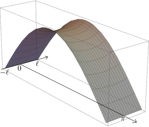 Figure 1
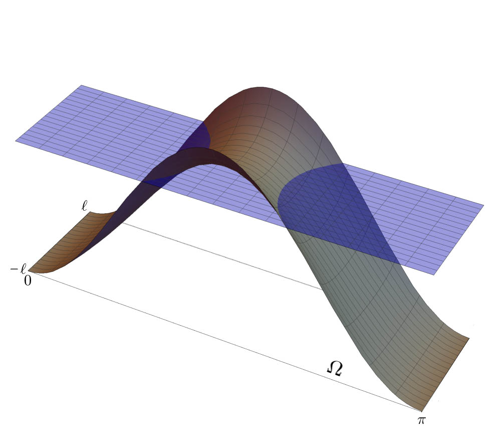 Figure 2
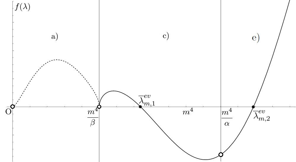 Figure 3
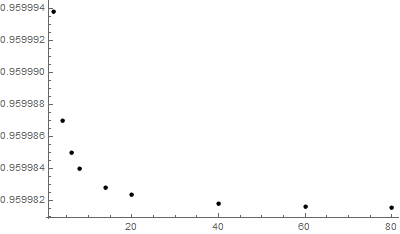 Figure 4
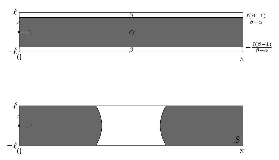 Figure 5
| Case | ||||||||||
|---|---|---|---|---|---|---|---|---|---|---|
| 0.960009 | 15.3610 | 77.767 | 245.798 | 600.145 | 1244.59 | 2306.05 | 3934.57 | 6303.42 | 9609.09 | |
| , | 0.959999 | 15.3599 | 77.759 | 245.755 | 599.982 | 1244.10 | 2304.82 | 3931.85 | 6297.92 | 9598.78 |
| , | 0.959982 | 15.3589 | 77.747 | 245.688 | 599.724 | 1243.34 | 2302.88 | 3927.53 | 6289.17 | 9582.33 |
Peer Reviews
No public reviews on file for this paper yet. If you reviewed it on a platform where reviews are public (OpenReview, ICLR, NeurIPS, ICML), you can paste yours below so the community can read it here.
Videos
No videos yet. Explain this paper in a talk, walkthrough, or lecture? Add one.
On the first frequency of reinforced
partially hinged plates
Elvise BERCHIO
Dipartimento di Scienze Matematiche,
Politecnico di Torino,
Corso Duca degli Abruzzi 24, 10129 Torino, Italy.
*E-mail address: *[email protected]
,
Alessio FALOCCHI
Dipartimento di Scienze Matematiche,
Politecnico di Torino,
Corso Duca degli Abruzzi 24, 10129 Torino, Italy.
*E-mail address: *[email protected]
,
Alberto FERRERO
Dipartimento di Scienze e Innovazione Tecnologica,
Universitá del Piemonte Orientale,
Viale Teresa Michel 11, Alessandria, 15121, Italy.
*E-mail address: *[email protected]
and
Debdip GANGULY
Indian Institute of Science Education and Research,
Dr. Homi Bhabha Road, Pashan, Pune 411008, India.
*E-mail addresses: *[email protected]
Abstract.
We consider a partially hinged rectangular plate and its normal modes. The dynamical properties of the plate are influenced by the spectrum of the associated eigenvalue problem. In order to improve the stability of the plate, we place a certain amount of denser material in appropriate regions. If we look at the partial differential equation appearing in the model, this corresponds to insert a suitable weight coefficient inside the equation. A possible way to locate such regions is to study the eigenvalue problem associated to the aforementioned weighted equation. In the present paper we focus our attention essentially on the first eigenvalue and on its minimization in terms of the weight. We prove the existence of minimizing weights inside special classes and we try to describe them together with the corresponding eigenfunctions.
Key words and phrases:
eigenvalues; plates; torsional instability; suspension bridges
2010 Mathematics Subject Classification:
35J40; 35P15; 74K20
1. Introduction
Following [16] one may view a bridge as a long narrow rectangular thin plate hinged at two opposite edges and free on the remaining two edges: this plate well describes decks of footbridges and suspension bridges which, at the short edges, are supported by the ground. We refer to the monograph [17] for a detailed survey of old and new mathematical models for suspension bridges. Up to scaling, we may assume that the plate has length and width with so that
[TABLE]
There is a growing interest of engineers on the shape optimization for the design of bridges and, in particular, on the sensitivity analysis of certain eigenvalue problems, see [19, Chapter 6]. As pointed out by Banerjee [3], the free vibration analysis is a fundamental pre-requisite before carrying out a flutter analysis. Whence, in the the stability analysis of the plate a central role is played by the following eigenvalue problem:
[TABLE]
where denotes the Poisson ratio of the material forming the plate. Throughout the paper we consider , a range of values that includes most of the elastic materials. The boundary conditions on the short edges tell that the plate is hinged; these conditions are attributed to Navier, since their first appearance in [23]. We refer to [4] for the derivation of (1) from the total energy of the plate. Note that in [16] the whole spectrum of (1) was determined, while in [6] the results were exploited to study the so-called torsional stability of suspension bridges for small energies. Furthermore, in [4] the variation of the eigenvalues, under domain deformations, which may not preserve the area, was investigated, see also [7] for related results about Dirichlet polyharmonic eigenvalue problems.
In the engineering literature the critical threshold for the wind velocity at which a form of dynamical instability, named flutter, arises, is commonly related to the distance between the square of the frequencies of certain oscillating modes. We refer to [4] for a discussion of possible formulas to compute the above mentioned threshold. In particular, it follows that a possible way to increase this threshold is by increasing the distance between eigenvalues. Having this goal in mind, in order to improve the stability of the plate, we study the effect of inserting a denser material within it. This can be modelled in mathematical terms by a suitable weight function ; for this reason we study the *weighted *eigenvalue problem:
[TABLE]
where, for with fixed, belongs to the following family of weights:
[TABLE]
The spectral analysis of (2) should indicate where to place the denser material within the plate. In this respect, the condition on the integral of is posed in order to make the comparison with the case consistent. It is worth mentioning that a related linear problem has been recently treated in [5], by studying the equation
[TABLE]
subject to the boundary conditions in (2), where is the characteristic function of and is a positive constant. The solution of this equation describes the vertical displacement of the plate under the action of a load and the weight is seen as an aerodynamic damper placed in in order to reduce the action of the external force. The spectral analysis of (2) can help to complete and enrich the results obtained in [5].
Coming back to (2), the natural starting point of the study is the investigation of the effect of on the first eigenvalue , namely to study:
[TABLE]
The minimization of the first eigenvalue for the second order Dirichlet version of (2), named composite membrane problem, has been studied in [8]-[11],[25], while the minimization of the first eigenvalue for the equation in (2) under Dirichlet or Navier boundary conditions, named composite plate problem, has been studied in [1],[2],[13]-[14]. Finally, we refer to [21] for a detailed stability analysis, upon variation of , of the weighted eigenvalues of general elliptic operators of arbitrary order subject to several kinds of homogeneous boundary conditions. In this field of research, typical results are existence of optimal pairs and their qualitative properties, such as symmetry or symmetry breaking. From this point of view a crucial obstruction, when passing from the membrane to the plate problem, namely from the second to the fourth order case, is represented by the loss of maximum and comparison principles which usually enter either in the study of the simplicity of the first eigenvalue and in the techniques applied to prove symmetry results, such as reflections methods or moving planes techniques. Nevertheless, a suitable choice of the boundary conditions (e.g. Navier or Steklov b.c.) or of the geometry of the domain (e.g. small perturbations of balls) may yield the validity of so-called positivity preserving property which basically means that solutions, of the associated linear problem, maintain the sign of data. Concerning problem (2), the difficulties in its analysis, are even increased by the choice of the unusual boundary conditions for which no positivity preserving property is known. As far as we are aware, the minimization of the first eigenvalue of problem (2) has not been considered in literature, hence the present paper represents the first contribution on this topic. In our analysis we take advantage of the fact that is a planar domain and, when restricting the class of weights, some explicit computations can be performed. On the other hand, we exploit a sort of restricted positivity preserving property with respect to the variable, that we prove in Theorem 3.8 below, having its own theoretical interest. We note that the above mentioned restriction on admissible weights is also justified by the applicative nature of our problem. Indeed, it is known that minimization problems, like the composite membrane problem, naturally lead to homogenization [22], see also [20] for a stiffening problem for the torsion of a bar. Homogenization would lead to optimal designs with reinforcements scattered throughout the structure, namely designs impossible to reproduce for engineers. In order to avoid homogenization, the class of admissible reinforcements should be sufficiently small. See also Nazarov-Sweers-Slutskij [24], where only “macro” reinforcements are considered, although in a fairly different setting.
As we have already remarked, in order to improve the stability of the plate, the final goal of the spectral analysis of problem (2) is to maximize the distance between selected oscillating modes. The present paper has to be meant as a first contribution in this direction and it should be hopefully followed by the optimization analysis of the higher eigenvalues. This, together with the further investigation of the positivity properties of the operator in (2), represents a promising topic of research that we plan to develop in our future studies.
The paper is organised as follows. Section 2 is devoted to the description of the notations and of some results about the case . In Section 3 one can find the main results of the paper which are proved in Sections 6 and 7. In Section 4 we show some numerical results on the behaviour of the eigenvalues which complement our theoretical analysis. Finally, in Section 5 we show the validity of a positivity preserving property for a one dimensional fourth order problem, coming from a suitable Fourier decomposition of solutions to the plate problem.
2. Notations and known results when
From now onward we fix with and . The natural functional space where to set problem (2) is
[TABLE]
is a Hilbert space when endowed with the scalar product
[TABLE]
and associated norm
[TABLE]
which is equivalent to the usual norm in , see [16, Lemma 4.1]. Then problem (2) may also be formulated in the following weak sense
[TABLE]
where belongs to the family of weights defined in (3) with and fixed. We point out that condition implies since . Moreover, we observe that it is not restrictive to assume when we focus our analysis on weights that do not coincide a.e. with the constant function . Indeed, if we assume that , it must be a.e. in since otherwise we would have ; similarly, if we assume that , it must be a.e. in . For this reason, since the aim of our research is to study the effect of a non constant weight on the first eigenvalue of (2), in what follows we will always assume .
The bilinear form is continuous and coercive and is positive a.e. in , therefore standard spectral theory of self-adjoint operators shows that the eigenvalues of (2) may be ordered in an increasing sequence of strictly positive numbers diverging to and that the corresponding eigenfunctions form a complete orthonormal system in .
Since by elliptic regularity the eigenfunctions are at least in Furthermore, the first eigenvalue is characterized by
[TABLE]
When the spectrum of (2) has been completely characterized. We recall the following statement from [16], including some refinements on the eigenvalues estimates proved in [4].
Proposition 2.1**.**
Let in (2). The set of eigenvalues of (2) may be ordered in an increasing sequence of strictly positive numbers diverging to and any eigenfunction belongs to ; the set of eigenfunctions of (2) is a complete system in . Moreover:
* for any , there exists a unique eigenvalue with corresponding eigenfunction*
[TABLE]
* for any and any there exists a unique eigenvalue satisfying*
**
and with corresponding eigenfunction
[TABLE]
* for any and any there exists a unique eigenvalue with corresponding eigenfunctions*
[TABLE]
* for any satisfying there exists a unique eigenvalue with corresponding eigenfunction*
[TABLE]
Finally, if
[TABLE]
then the only eigenvalues are the ones given in .
In the following, to avoid too many distinctions, we will always assume that (6) holds.
By Proposition 2.1 and [16, Section 7] it is readily deduced that the first eigenvalue of problem (2) with is , namely , it is simple and up to constant multiplier the first eigenfunction is given by
[TABLE]
Hence, is positive in , convex in the variable and concave in the variable.
3. Main results
As in Section 2 we always assume
[TABLE]
Then, recalling (3), we focus on the infimum problem
[TABLE]
where is defined in (5).
Definition 3.1**.**
A couple is called optimal pair if achieves the infimum in (8) and is an eigenfunction of .
Adapting to our case [9, Theorem 13] and [13, Theorem 1.4], we show that there exists an optimal pair for problem (8) and and are suitably related. Using the language of the control theory we find that is a bang-bang function; more precisely we prove
Theorem 3.2**.**
There exists and optimal pair . Furthermore, and are related as follows
[TABLE]
where and are the characteristic functions of the sets and and is such that and for some .
Theorem 3.2 states that the plate has to be made of two materials, but it gives no information about the location of the materials and hence, no practical information on how to build the plate. To this aim, a more explicit suggestion is provided by the following
Proposition 3.3**.**
Let satisfy one of the following assumptions
- (i)
* is even and there exists such that*
[TABLE]
- (ii)
* is symmetric with respect to the line and there exists such that*
[TABLE]
Then,
[TABLE]
where is as defined in Proposition 2.1-(i).
Remark 3.4**.**
The same idea of the proof of Proposition 3.3-(i) can be repeated to prove that (10) holds if satisfies
- (iii)
* is even and there exist points such that*
[TABLE]
for all .
Since the weights considered in Proposition 3.3 prove to be effective in lowering the first frequency of (1), by combining Proposition 3.3 with Theorem 3.2, we include in the list of candidate solutions to problem (8) the weights:
[TABLE]
and
[TABLE]
In Section 4 we obtain numerically a positive eigenfunction, denoted by , corresponding to with as in (11). In Figure 1 on the left, we plot and we use it to determine qualitatively what should be the set predicted by Theorem 3.2. In Figure 1 on the right we compare the weight in (9) (bottom), with this choice of the set , and the weight (top). From these plots we infer that is not a theoretical optimal pair of (8).
On the other hand, in Theorem 3.5 below we prove that belongs to an optimal pair if we properly restrict the class of admissible weights to a suitable subset of .
Theorem 3.5**.**
Let us define
[TABLE]
When the following statements hold:
if and there exists such that
[TABLE]
then
[TABLE]
we have
[TABLE]
where is as defined in (11).
Remark 3.6**.**
Concerning the meaning of the upper bound in Theorem 3.5 a couple of remarks are in order. The proof of Theorem 3.5 is achieved by studying a family of related 1-dimensional eigenvalue problems. Indeed, any eigenfunction of (2) can be expanded in Fourier series as follows
[TABLE]
with and, if , for every fixed, satisfies the weak form of the problem:
[TABLE]
See Section 7 for the details. In particular, if we denote by the first eigenvalue of (2) and by the first eigenvalue of (12) with fixed, assumption ensures that
[TABLE]
see Lemma 7.1 below. On the other hand, the condition allows to prove that the first eigenfunction of is monotone in , and this information yields the comparison between weights of Theorem 3.5-, see Lemma 7.3. The numerical results we state in Section 4 suggest that both the upper bounds on are merely technical conditions.
It is worth noting that, in order to lower the first eigenvalue of under Dirichlet or Navier boundary conditions, since the eigenfunctions vanish on the boundary, one expects that the weight is more effective if it achieves its lowest value close to the boundary, see e.g. [13, Theorem 1.5]. Theorem 3.5 shows that the partially hinged boundary conditions lead to a complete different situation since the weight achieves its lowest value far from the free long edges, see Figure 1 on the right (top). This behaviour is somehow related to the monotonicity of the first eigenfunction, as shown by Theorem 3.7 below, cfr. Figure 2.
Theorem 3.7**.**
Let be the family of weights defined in Theorem 3.5 with . Then, for any the first eigenvalue of (4) is simple. Furthermore, if is an eigenfunction of then is of one sign in and moreover can be written as with even and strictly monotone in .
Unfortunately, the above statement does not carry over to all weights . This is related to the well-know loss of comparison principles for fourth order elliptic operators. Indeed, the proof of Theorem 3.7 strongly relies on a sort of restricted positivity preserving property with respect to the variable that we prove by separating variables. More precisely, we have
Theorem 3.8**.**
Let be an integer. Furthermore, let be the weak solution to the problem
[TABLE]
namely
[TABLE]
Then, for some and the following implication holds
[TABLE]
4. Numerical Results
In this section, for any , we compute numerically the first eigenvalue of problem (12) with as defined in (11). More precisely, we take
[TABLE]
with and , so that . In terms of engineering applications, this means that we are dealing with a weight given by the pairing of two materials having different densities and , properly placed on rectangular strips, having the length of the whole plate. Furthermore, we assume that the deck of the bridge is composed by a mixture of concrete and steel, hence the Poisson ratio is variable between 0.15 and 0.3; for this reason in what follows we take .
Note that, since is an even function, to determine all eigenvalues of (12), we may focus on even and odd eigenfunctions. Indeed, if is an eigenfunction which is neither odd or even, it is readily verified that also and are eigenfunctions, respectively even and odd, corresponding to the same eigenvalue of . On the other hand, since the first eigenvalue of (12) is simple and the corresponding eigenfunctions are of one sign in , see Remark 3.6 and Theorem 3.7, we infer that must be an even function, whence to compute we may concentrate on even eigenfunctions that we named . For any we have that
[TABLE]
where and satisfy:
[TABLE]
Note that the compatibility conditions between the functions and , ensure that , while come from and its regularity. Clearly, the analytical expression of and depends on the roots of the characteristic polynomials related to the first two equations in (15); we denote them respectively by and and we find that they satisfy
[TABLE]
Therefore, the sign of and determines different kinds of solutions. We introduce the following notations
[TABLE]
and we distinguish five cases:
- a)
, implying and
[TABLE]
- b)
, so that , and
[TABLE]
- c)
, implying and
[TABLE]
- d)
, so that , and
[TABLE]
- e)
, implying and
[TABLE]
The six coefficients involved in the definition of and can be determined, in each of the five cases, by imposing the boundary and compatibility conditions. We present here only case c), since the others cases can be treated similarly.
First of all we assume that satisfies the boundary conditions, i.e.
[TABLE]
then we impose the compatibility conditions, i.e.
[TABLE]
We should solve a system of six equations and six unknowns; through some algebraic manipulations, we reduce it to a system of four equations and four unknowns . More precisely, we get
[TABLE]
To system (16) we associate a square matrix depending on the eigenvalues , hence (16) rewrites ; since we are interested in not trivial solutions we end up with the equation
[TABLE]
In this way, for any fixed, the zeroes of the function in the interval , if they exist, are the eigenvalues corresponding to eigenfunctions as in (14) with and as in c). This procedure can be applied to each of the five cases .
The computation by hand of (17) is very involved, thus we perform it numerically in all the five cases listed above. Our experiments reveal that cases b) and d) do not occur if , for a suitable which, for all tested values of and , satisfies . This implies large for small , as common in plates for bridges. Therefore, we focus on cases a)-c)-e).
We tested several values of and always obtaining the same qualitative plot of . Figure 3 shows the following facts: we do not find eigenvalues in case a), since for all ; the first eigenvalue falls always in case c); all the other eigenvalues corresponding to even functions fall in case e). Furthermore, our numerical results yield the following bounds on eigenvalues corresponding to even eigenfunctions:
[TABLE]
We are now interested in checking if (13) holds when the upper bound on of Theorem 3.5 is not satisfied (see also Lemma 7.1 below), i.e. if
[TABLE]
when . To this aim we study the behaviour of the maps and . In Figure 4 we plot some points of the map for , we register a similar behaviour for with . On the other hand, in Table 1 we put the values of for , computed taken , and for two suitable choices of and with satisfying or not the smallness assumption on of Theorem 3.5.
All the numerical experiments performed suggest that
[TABLE]
and the trend does not change varying and . In particular, the above lower bound for does not depend on and, jointly with the fact that , supports the conjecture that
[TABLE]
for any , hence the assumption of Theorem 3.5 seems a merely technical condition.
5. A positivity preserving property
In this section we state and prove some results about a positivity preserving property for the fourth order differential operator
[TABLE]
subject to the boundary conditions:
[TABLE]
As in Section 3 we fix . These results have their own independent interest and will be exploited in the proofs of Section 7.
For every , it will be convenient to consider the following scalar product in :
[TABLE]
which defines an equivalent norm in that we will denote by .
Theorem 5.1**.**
Let be an integer and let . Furthermore, assume that is a weak solution to the problem
[TABLE]
namely
[TABLE]
where is defined in (19). Then the following implication holds
[TABLE]
Hence, the operator defined in (18), under the boundary conditions in (20), satisfies the positivity preserving property.
As a consequence of Theorem 5.1 we have
Corollary 5.2**.**
Let , be an integer. Furthermore, set and assume that satisfies
[TABLE]
where is defined in (19). Then
[TABLE]
Proof.
Let and let be the unique solution to
[TABLE]
By Theorem 5.1, . Inserting in (22) we infer
[TABLE]
Hence, in . By contradiction, assume that in . Then, if , we have that the characteristic function of satisfies and . Let now satisfy
[TABLE]
Since, by elliptic regularity, and, by Theorem 5.1, in , we deduce that for every there exist : and in . Furthermore, by definition of we have
[TABLE]
Combining this with (22), we deduce
[TABLE]
and
[TABLE]
Namely,
[TABLE]
Taking in the above inequality we conclude in and the proof follows. ∎
We conclude this section with the proof of Theorem 5.1.
Proof of Theorem 5.1.
The proof follows by a direct inspection of the sign of the unique solution to (21). First we note that, for fixed and , all solutions to the equation
[TABLE]
where denotes the trivial extension of to , write
[TABLE]
with and
[TABLE]
where
[TABLE]
Exploiting the regularity of , it follows that all the above solutions belong to (the regularity can be improved by increasing the regularity of ); the thesis can be reached proving that
[TABLE]
since .
If we fix the constants in such a way that:
[TABLE]
then the restriction of to , that we will still denote with , is the unique solution to (21). More precisely, by imposing the above conditions we obtain the system
[TABLE]
which decouples in the following two systems
[TABLE]
[TABLE]
By setting
[TABLE]
[TABLE]
[TABLE]
[TABLE]
[TABLE]
[TABLE]
the solutions to the above systems write
[TABLE]
[TABLE]
[TABLE]
[TABLE]
By exploiting the symmetry of , for and , we have
[TABLE]
while, for and , we have
[TABLE]
where and denotes, respectively, the -th derivate of and of . Hence,
[TABLE]
and
[TABLE]
First of all we study the sign of the coefficients and . Since , has the same sign of
[TABLE]
[TABLE]
[TABLE]
[TABLE]
We observe that
[TABLE]
for and for all , implying that (25) is positive; about the sign of (24) we introduce the map
[TABLE]
and we compute its derivative
[TABLE]
Thanks to (26), for we obtain so that is always positive () and in particular . The sign of depends on
[TABLE]
[TABLE]
that, applying again (26), gives for all and .
For our purposes we need to compare the absolute value of and ; since the sign of is not known a priori, we study the sign of , i.e.
[TABLE]
Recalling that , we obtain the positivity of
[TABLE]
thus if
[TABLE]
the achievement follows from the positivity of \big{(}\cosh(z)\mp\sinh(z)\big{)}\big{(}2\pm(1+\sigma)\big{)} for all and .
Fixed , we set
[TABLE]
and we focus on the qualitative behaviour of where, from above, , and . Clearly, is continuous and differentiable on , moreover
[TABLE]
This fact implies that has at least two zeros of opposite sign on ; we prove now that has exactly two distinct zeros on .
We know that if and only if
[TABLE]
Computing we observe that
[TABLE]
This follows because is always decreasing on ; indeed , so that . Moreover for . Now let us suppose for contradiction that has more than two zeros on , for instance it has 3 distinct zeros ; this implies that has 3 distinct zeros, then, the Rolle’s Theorem applied to in the intervals and ensures the existence of at least two points in which on and this contradicts (27). Hence, , and in turn also , has exactly two zeros of opposite sign on .
Since has exactly two zeros of opposite sign on and , if we prove that the thesis follows. To this aim we study the sign of , in particular we consider
[TABLE]
where
[TABLE]
The final part of the proof is devoted to prove that the coefficients and are positive. We recall that
[TABLE]
and we introduce four maps related respectively to the previous coefficients
[TABLE]
Thanks to (26) , and are always positive for and for all . The same conclusion holds for the maps , due to the following inequality
[TABLE]
This completes the proof.
6. Proof of Theorem 3.2 and Proposition 3.3
6.1. Proof of Theorem 3.2
We start with the existence issue.
Lemma 6.1**.**
The infimum in (8) is achieved.
Proof.
Let be a minimizing sequence for , i.e.
[TABLE]
Furthermore, let be a (normalized) eigenfunction to , namely and This immediately implies for some positive constant Therefore, using the compact embedding of we can extract two subsequences, still denoted by such that
[TABLE]
[TABLE]
Moreover, implies and therefore up to a subsequence, in as so that also satisfies the integral condition in (3). Since strongly closed convex sets are weakly closed, we infer that a.e. in . Hence, . On the other hand, we obtain
[TABLE]
where we have exploited the fact that since is a planar domain. In particular, we conclude that Furthermore,
[TABLE]
Whence
[TABLE]
Therefore, the couple is an optimal pair and ; this completes the proof.
∎
To problem (8) we associate the following infimum problem
[TABLE]
where is as in (8) and
[TABLE]
The proof of Lemma 6.1 with minor changes shows that also problem (28) admits an optimal pair . Furthermore, there is an one-to-one correspondence between problems (8) and (28). Indeed, to any we can associate by setting
[TABLE]
Clearly and
[TABLE]
Viceversa to any we can associate by setting
[TABLE]
Clearly and Furthermore, we have
Lemma 6.2**.**
Let and be as defined in (8) and in (28). There holds
[TABLE]
Proof.
We shall prove the lemma in two steps.
Step 1 : Let and such that is achieved for this optimal pair and let . Clearly we have
[TABLE]
Step 2 : Let now and with i.e., Then for any
[TABLE]
Since, implies for any and , passing to the infima, (29) yields
[TABLE]
This completes the proof. ∎
Finally, we prove that the optimal pair of problem (28) can be characterised as follows
Lemma 6.3**.**
Let be an optimal pair of problem (28). Then, and are related as follows
[TABLE]
where is the characteristic function of a set such that and
[TABLE]
for some .
Proof.
The proof is along the line of [13, Proposition 3.3]. For the sake of completeness we shall outline the main ideas.
Step 1. Let be such that and consider the functional
[TABLE]
We prove that the infimum problem
[TABLE]
admits a solution where is such that and satisfies one of the following
[TABLE]
where is defined as
[TABLE]
Let be as above, then and one obtains
[TABLE]
On the other hand we claim that the following inequality holds
[TABLE]
If this is true then one immediately obtain and this concludes the proof of step 1.
We prove the validity of the claim by considering the cases and separately.
If , we argue as follows
[TABLE]
If the proof follows with minor changes.
Step 2. We prove that if is an optimal pair as in the statement of the lemma and if is the corresponding set defined according to Step 1, then is still an optimal pair.
Set
[TABLE]
Since we have
[TABLE]
On the other hand, letting an optimal pair as in the statement of the lemma, from Step 1 we have
[TABLE]
and therefore
[TABLE]
This proves that
[TABLE]
and in particular that is an optimal pair.
Step 3. Let be the optimal pair introduced in Step 2 and let be the number in (30) corresponding to . Let
[TABLE]
We prove that and that .
Suppose by contradiction that . Since we can write the Euler-Lagrange equation related to (28) almost everywhere and we have
[TABLE]
Since satisfies the partially hinged boundary conditions this means that it must be one of the eigenfunctions listed in Proposition 2.1 which is impossible since the set of zeroes of any of the eigenfunctions of Proposition 2.1 has zero measure thus contradicting the definition of which forces to be a set of positive measure. This proves that .
Suppose now by contradiction that , we have that
[TABLE]
Now, exploiting the fact that is constant in and , we infer
[TABLE]
and hence, since a.e. in and , we obtain and this is absurd.
Step 4. We complete the proof of the lemma. First of all, we observe that by Step 3, it is not restrictive, up to a set of zero measure, to assume that in such way that and, in turn,
[TABLE]
It remains to prove that a.e. in . Since and are both optimal pairs we have
[TABLE]
thus implying that
[TABLE]
It is easy to check that a.e. in being . In order to prove that a.e. in , we apply (32) to , and observing that the inequality (32) is an equality being and both optimal pairs. In particular we have that
[TABLE]
which implies
[TABLE]
But the function in , as one can deduce by (33), and hence by (34) we conclude that a.e. in the same set.
We have so proved that a.e. in and this completes the proof of the lemma. ∎
Proof of Theorem 3.2 completed.
The existence of an optimal pair follows from Lemma 6.1. If we put by Lemma 6.2 we deduce that is an optimal pair for . Moreover by Lemma 6.3 we also have that a.e. in with and as in (31). Hence we conclude that
[TABLE]
6.2. Proof of Proposition 3.3.
We prove the two statements separately.
Proof of Proposition 3.3-(i).
We know that the function introduced in (7) is an eigenfunction corresponding to the least eigenvalue of (2) with . Furthermore,
[TABLE]
Now, by exploiting the fact that is even and increasing in and is even, we deduce that
[TABLE]
where in the last step we have exploited the fact that , therefore . Hence,
[TABLE]
From the above inequality we infer
[TABLE]
and the proof of the statement follows.
Proof of Proposition 3.3-(ii).
The idea of the proof is similar to that applied to prove statement . By exploiting the fact that and for all , we deduce that
[TABLE]
where in the last step we have exploited the assumption , hence . From the above inequality the proof follows as for statement .
7. Proof of Theorem 3.5, Theorem 3.7 and Theorem 3.8
In this section we restrict the admissible weights to the family defined in Theorem 3.5. Clearly, for all . Furthermore, for positive integer, will denote the scalar product in defined in (19) with equivalent norm .
Let be an eigenfunction of (4), its Fourier expansion reads
[TABLE]
with since (at least). Inserting in (4), we get that, for every fixed, satisfies the equation
[TABLE]
which is the weak formulation of the problem (12). Notice that, by elliptic regularity, any solution of (12) , lies in . Hence, the boundary conditions in (12) are satisfied pointwise. Since the bilinear form is continuous and coercive the eigenvalues of problem (35) may be ordered in an increasing sequence of strictly positive numbers diverging to and the corresponding eigenfunctions form a complete system in . Whence, for what remarked so far, when there is a one to one correspondence between eigenvalues of (35) and eigenvalues of (4). In particular, if we denote by the first eigenvalue of (4) and by the first eigenvalue of (35) with fixed, namely
[TABLE]
it is natural to conjecture that
[TABLE]
Unfortunately, for fixed, due to the negative terms in the norm , the monotonicity of is not easy to detect and we do not have a proof of the above equality for general ; in Section 4 we give some suggestions through numerical experiments. Nevertheless, we have the following partial result
Lemma 7.1**.**
*If then *
[TABLE]
where the are the numbers defined in Proposition 2.1-(i).
If furthermore , then
[TABLE]
Proof.
Let
[TABLE]
From Proposition 2.1 it is readily deduced that is an eigenfunction corresponding to the least eigenvalue of (35) with and fixed (otherwise we will find an eigenvalue of (2) not included in those listed in Proposition 2.1). Furthermore,
[TABLE]
Now, by exploiting the fact that is even and increasing in , the first part of the proof follows with the same argument of Proposition 3.3-(i), hence we omit it.
Next we turn to the second estimate. Let be an eigenfunction corresponding to the least eigenvalue of (35), with fixed and with satisfying the assumption of Lemma 7.1. In particular, , with as given above. Since for every , we get
[TABLE]
Then, the thesis follows by recalling that, from Proposition 2.1-(i), for every and from the first part of the proof . ∎
Hence, under the assumptions of Lemma 7.1, we have
[TABLE]
In particular, the weights considered in Lemma 7.1 prove to be effective in lowering the first frequency of (2), which is one of the main goal of the present analysis. In the following we refine the result by carrying on a more deeper analysis. First we note that, from above, if is an eigenfunction of , then is an eigenfunction of . Therefore, and have the same sign.
We now discuss the sign of and the simplicity of in
Lemma 7.2**.**
Let integer fixed and let . Then, the first eigenvalue of problem (35) is simple and the first eigenfunction is of one sign in .
Furthermore, if the same conclusion holds for the first eigenvalue of (4), namely it is simple and the corresponding eigenfunction is given by , hence of one sign in .
Proof.
We apply the decomposition with respect to dual cones technique, see [18, Chapter 3] suitably combined with Theorem 5.1. Let and let be its dual cone, namely
[TABLE]
where is defined in (19). Then, for any there exists a unique such that
[TABLE]
Now we know that
[TABLE]
For contradiction, assume that changes sign. Then, we may decompose with and .
In the remaining part of this proof we need some results on a positivity preserving property which is treated in Section 5.
From Corollary 5.2, we deduce that in . Then, replacing with , exploiting the fact that in and the orthogonality of and in , we infer
[TABLE]
a contradiction. Hence in and since solves (35), by Theorem 5.1 with , we conclude that in .
The simplicity follows by noting that if and are two linearly independent positive minimizers, then is a sign-changing minimizer for some suitably chosen, a contradiction. ∎
Next we focus on the sign of and we prove
Lemma 7.3**.**
If is such that and if is a positive eigenfunction of (35) with corresponding to the first eigenvalue , then is increasing in .
Proof.
For shortness we will write instead of . Since is even, being positive, we infer that it is an even function. Hence, since it satisfies .
If is continuous, then and it satisfies the equation in (12) pointwise. We recall that the boundary conditions in (12) are satisfied pointwise also when is not continuous. Since is positive, and, by Lemma 7.1, we know that , from the equation we infer
[TABLE]
If is not continuous, since only a finite number of points of jump discontinuity are allowed in , say for some integer , the above inequality holds in each interval . Furthermore, for any , the right and left fourth order derivative at exists and they are given by .
First we show that
[TABLE]
By contradiction, let be such that . Since and , there exists such that and, by (37), . Next the following two cases may occur.
CASE 1: . From above, is negative and, in turn, also is negative in a right neighborhood of . Since the boundary conditions in (12) yield , we infer that there exists such that , and in . Whence, by (37), in or in each of the subintervals contained in . Since is continuous in , in any case, we have that it is strictly decreasing in , hence in in contradiction with .
CASE 2: . We distinguish two further cases.
CASE 2a: . By (37), , hence in a right neighborhood of [math]. Then, since , there exists such that in and . In turn, in and by (37) in (or in each of the subintervals contained in ). Since is continuous this implies that it is strictly decreasing in . Since , we infer , a contradiction.
CASE 2b: . From and we infer that is negative in a left neighborhood of . Then, since , there exists such that in and . In turn, recalling that , there exists such that and, by (37), we infer that in , in contradiction with .
Next we come back to the proof of the statement. By (38) we know that either in or in .
Assume that in , then . Indeed, if , since , then is positive in a right neighborhood of [math], a contradiction. From , together with (37) and , it follows that is negative in a right neighborhood of [math] and, in turn, also is negative in a right neighborhood of [math]. Since, from the boundary conditions , we deduce that there exists such that , and in . But then, from (37), is strictly decreasing in and, recalling that we reach a contradiction. ∎
All the above statements yield the proof of Theorem 3.5.
Proof of Theorem 3.5 completed.
The key point is to note that, by Lemma 7.3, we have
[TABLE]
Indeed, since by (39) is increasing in , to prove we may argue as in the proof of the first part of Lemma 7.1 with instead of . In particular, we readily infer that and since, from Lemma 7.1, for all , the proof of follows.
Next we prove . Set , for every there holds
[TABLE]
Then, we may argue again as in the proof of the first part of Lemma 7.1 with instead of and conclude
[TABLE]
Once more, from Lemma 7.1, for all and the statement of Theorem 3.5 follows.
Proof of Theorem 3.7.
The proof readily follows by combining the statements of Lemma 7.2 and Lemma 7.3.
Proof of Theorem 3.8.
The proof readily follows as a corollary of Theorem 5.1 by exploiting the same separation of variables performed in the Proof of Theorem 3.5.
Acknowledgments. The authors are grateful to the anonymous referee whose relevant comments and suggestions helped in improving the exposition of the preliminary form of the manuscript. The first three authors are members of the Gruppo Nazionale per l’Analisi Matematica, la Probabilità e le loro Applicazioni (GNAMPA) of the Istituto Nazionale di Alta Matematica (INdAM) and are partially supported by the INDAM-GNAMPA 2019 grant “Analisi spettrale per operatori ellittici con condizioni di Steklov o parzialmente incernierate” and by the PRIN project “Direct and inverse problems for partial differential equations: theoretical aspects and applications” (Italy). The third author was partially supported by the INDAM-GNAMPA 2018 grant “Formula di monotonia e applicazioni: problemi frazionari e stabilità spettrale rispetto a perturbazioni del dominio” and by the research project “Metodi analitici, numerici e di simulazione per lo studio di equazioni differenziali a derivate parziali e applicazioni” Progetto di Ateneo 2016, Università del Piemonte Orientale “Amedeo Avogadro”. The research of the fourth author is partially supported by an INSPIRE faculty fellowship (India).
The reference list from the paper itself. Each links out to its DOI / PubMed record.
- 1[1] C. Anedda, F. Cuccu, Steiner symmetry in the minimization of the first eigenvalue in problems involving the p-Laplacian , Proc. Amer. Math. Soc. 144, (2016), 3431–3440.
- 2[2] C. Anedda, F. Cuccu, G. Porru, Minimization of the first eigenvalue in problems involving the bi-laplacian , Rev. Mate. Teor. Appl. 16, (2009), 127–136.
- 3[3] J. R. Banerjee, A simplified method for the free vibration and flutter analysis of bridge decks , J. Sound Vibration 260 (2003), 829–845.
- 4[4] E. Berchio, D. Buoso, F. Gazzola, On the variation of longitudinal and torsional frequencies in a partially hinged rectangular plate , ESAIM Control Optim. Calc. Var. 24 (2018), 63–87.
- 5[5] E. Berchio, D. Buoso, F. Gazzola, D. Zucco, A Minimaxmax Problem for Improving the Torsional Stability of Rectangular Plates , J. Optim. Theory Appl. 177 (2018), 64–92.
- 6[6] E. Berchio, A. Ferrero, F. Gazzola, Structural instability of nonlinear plates modelling suspension bridges: mathematical answers to some long-standing questions , Nonlin. Anal. Real World Appl. 28 (2016), 91–125.
- 7[7] D. Buoso, P. D. Lamberti, Eigenvalues of polyharmonic operators on variable domains , ESAIM: Control, Optim. Calc. Var., 19, (2013), n.4, 1225–1235.
- 8[8] S. Chanillo, Conformal geometry and the composite membrane problem , Anal. Geom. Metr. Spaces 1 (2013), 31–35.