Simulation-based Value-at-Risk for Nonlinear Portfolios
Junyao Chen, Tony Sit, Hoi Ying Wong

TL;DR
This paper introduces a simulation-based method for estimating Value-at-Risk in nonlinear portfolios, improving accuracy and convergence over traditional approaches, especially for complex derivatives.
Contribution
It proposes a generic, model selection-enhanced simulation algorithm for VaR estimation applicable to high-dimensional, nonlinear portfolios with American-style derivatives.
Findings
Faster convergence of the new VaR estimation method.
Effective handling of high-dimensional, nonlinear derivative portfolios.
Improved accuracy over traditional delta-normal approaches.
Abstract
Value-at-risk (VaR) has been playing the role of a standard risk measure since its introduction. In practice, the delta-normal approach is usually adopted to approximate the VaR of portfolios with option positions. Its effectiveness, however, substantially diminishes when the portfolios concerned involve a high dimension of derivative positions with nonlinear payoffs; lack of closed form pricing solution for these potentially highly correlated, American-style derivatives further complicates the problem. This paper proposes a generic simulation-based algorithm for VaR estimation that can be easily applied to any existing procedures. Our proposal leverages cross-sectional information and applies variable selection techniques to simplify the existing simulation framework. Asymptotic properties of the new approach demonstrate faster convergence due to the additional model selection…
Click any figure to enlarge with its caption.
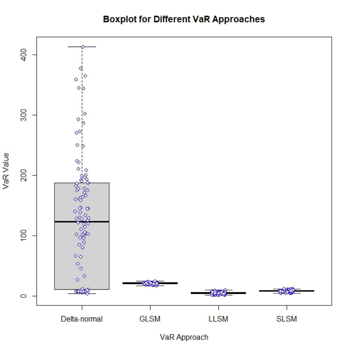 Figure 1
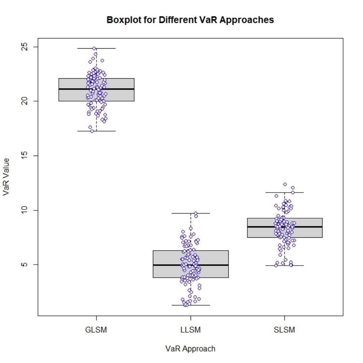 Figure 2
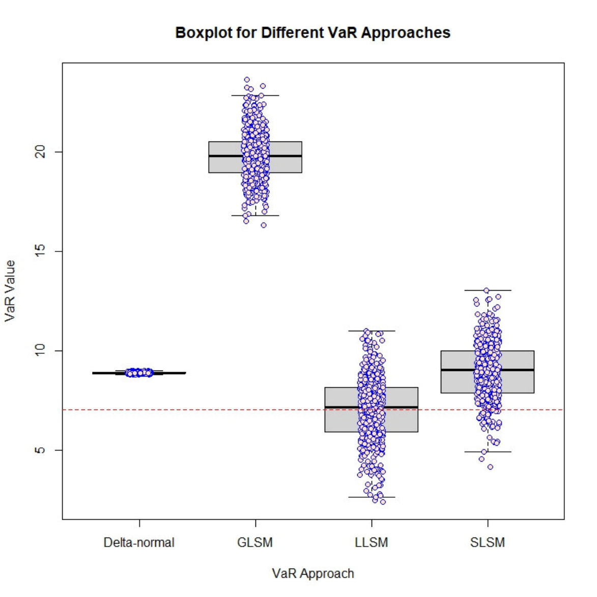 Figure 3
| Mean | Median | Standard Deviation | Back Testing | Time (in seconds) | |
|---|---|---|---|---|---|
| LSM | 1.78698 | 1.78664 | 0.11482 | 0.0290 | 18.62 |
| LLSM | 1.61693 | 1.61108 | 0.10932 | 0.0442 | 20.25 |
| Delta-normal† | 1.74591 | 1.74591 | - | 0.0329 | 7.62 |
| Delta-gamma† | 5.00858 | 5.00858 | - | 0 | 66.36 |
| Oracle | 1.58089 | 1.58089 | - | 0.0483 | 163,850 |
| Oracle† | 1.56778 | 1.56778 | - | 0.0500 | 3,634 |
| Mean | Median | Standard Deviation | Back Testing | Time (in seconds) | |
|---|---|---|---|---|---|
| SLSM | 8.94452 | 9.02583 | 1.45876 | 0.0200 | 13.07 |
| GLSM | 19.8179 | 19.8070 | 1.23116 | 0.0000 | 17.25 |
| LLSM | 7.02251 | 7.15271 | 1.62806 | 0.0505 | 25.16 |
| Delta-normal | 8.88734 | 8.88922 | 3.45005 | 0.0208 | 285.78 |
| Oracle | 7.04185 | 7.04185 | - | 0.0500 | 242,200 |
| Mean | Median | SD | Time (in seconds) | |
|---|---|---|---|---|
| SLSM | 8.38623 | 8.48900 | 1.59813 | 195.00 |
| GLSM | 21.0271 | 21.1145 | 1.51290 | 226.62 |
| LLSM | 5.01065 | 4.98452 | 1.86820 | 270.01 |
| Delta-normal | 189.649 | 7.87119 | 371.980 | 8,807.50 |
| Time | =year 2 | =day 10 | ||||
|---|---|---|---|---|---|---|
| Mean | Median | SD | Mean | Median | SD | |
| SLSM | 72.975 | 72.946 | 0.85212 | 69.517 | 69.489 | 0.81175 |
| GLSM | 75.391 | 72.946 | 0.86740 | 71.819 | 71.707 | 0.82638 |
| LLSM | 73.452 | 73.426 | 0.87146 | 69.971 | 69.946 | 0.83018 |
| Stopping Times | SLSM | GLSM | LLSM |
|---|---|---|---|
| 1 | 8.79705 | 19.7843 | 6.87493 |
| 4 | 8.54725 | 21.9728 | 6.06602 |
| 6 | 8.31433 | 22.8349 | 5.69590 |
| 8 | 8.17318 | 22.9505 | 5.36403 |
| 10 | 8.04154 | 22.9719 | 5.08469 |
| 12 | 7.92492 | 22.7725 | 4.97697 |
| 14 | 7.81349 | 22.6823 | 4.91529 |
| 16 | 7.76497 | 22.6077 | 4.84343 |
| 18 | 7.75723 | 22.5957 | 4.81491 |
| 80.38723 | 1.1015E-06 | 0.0085263 |
| 42.70244 | 1.5939E-06 | 0.0093093 |
| 67.57745 | 3.4755E-06 | 0.0024763 |
| 85.70454 | 3.8621E-05 | 0.0021646 |
| 58.11831 | 8.6745E-05 | 0.0042942 |
| 32.29635 | 7.4338E-05 | 0.0025601 |
| 57.28909 | 9.0098E-05 | 0.0044424 |
| 68.65604 | 1.1443E-05 | 0.0010326 |
| 86.43502 | 7.7736E-05 | 0.0016128 |
| 81.60649 | 1.2489E-05 | 0.0013172 |
| 1.00000 | 0.55000 | 0.29311 | 0.28272 | 0.23681 | 0.33050 | 0.34773 | 0.39159 | 0.29665 | 0.23986 | |
| 0.55000 | 1.00000 | 0.28613 | 0.27540 | 0.37854 | 0.38001 | 0.25678 | 0.32052 | 0.26683 | 0.28365 | |
| 0.29311 | 0.25510 | 1.00000 | 0.31191 | 0.39619 | 0.32266 | 0.27440 | 0.26772 | 0.39976 | 0.28598 | |
| 0.28613 | 0.33050 | 0.27440 | 1.00000 | 0.25510 | 0.23745 | 0.22811 | 0.25273 | 0.22504 | 0.35783 | |
| 0.28273 | 0.38001 | 0.22811 | 0.25273 | 1.00000 | 0.24183 | 0.25727 | 0.29702 | 0.30817 | 0.33151 | |
| 0.27540 | 0.32266 | 0.25727 | 0.29702 | 0.39976 | 1.00000 | 0.25681 | 0.21482 | 0.32993 | 0.20017 | |
| 0.31191 | 0.23745 | 0.25681 | 0.21482 | 0.22504 | 0.21862 | 1.00000 | 0.28263 | 0.29389 | 0.24210 | |
| 0.23681 | 0.24183 | 0.39159 | 0.28263 | 0.30817 | 0.23986 | 0.35783 | 1.00000 | 0.21862 | 0.23128 | |
| 0.37854 | 0.34773 | 0.32052 | 0.29665 | 0.32993 | 0.28365 | 0.33151 | 0.24210 | 1.00000 | 0.37021 | |
| 0.39619 | 0.25678 | 0.26772 | 0.26683 | 0.29389 | 0.28598 | 0.20017 | 0.23128 | 0.37021 | 1.00000 |
Peer Reviews
No public reviews on file for this paper yet. If you reviewed it on a platform where reviews are public (OpenReview, ICLR, NeurIPS, ICML), you can paste yours below so the community can read it here.
Videos
No videos yet. Explain this paper in a talk, walkthrough, or lecture? Add one.
Simulation-based Value-at-Risk for Nonlinear Portfolios
Junyao Chen, Tony Sit and Hoi Ying Wong
*Department of Statistics, The Chinese University of Hong Kong
[email protected] [email protected] [email protected]*
Abstract
Value-at-risk (VaR) has been playing the role of a standard risk measure since its introduction. In practice, the delta-normal approach is usually adopted to approximate the VaR of portfolios with option positions. Its effectiveness, however, substantially diminishes when the portfolios concerned involve a high dimension of derivative positions with nonlinear payoffs; lack of closed form pricing solution for these potentially highly correlated, American-style derivatives further complicates the problem. This paper proposes a generic simulation-based algorithm for VaR estimation that can be easily applied to any existing procedures. Our proposal leverages cross-sectional information and applies variable selection techniques to simplify the existing simulation framework. Asymptotic properties of the new approach demonstrate faster convergence due to the additional model selection component introduced. We have also performed sets of numerical results that verify the effectiveness of our approach in comparison with some existing strategies.
Keywords: Value-at-Risk, least-squares Monte Carlo, American-type derivatives, high dimensional portfolios
Introduction
One of the everyday challenges that financial institutions faces is re-evaluation of values and/or risk levels of their portfolios that mature some time in the future, which can generally be expressed in the form of
[TABLE]
where denotes the time, is a deterministic payoff function evaluated at the underlying asset value , denotes a risk-neutral probability measure with respect to and is a family of stopping times. The filtration up to time is denoted as . More importantly, based on these valuations, financial institutions need to calculate regulatory capitals in order to fulfill the requirements specified in Basel II for the banking industry BIS (2013) or Solvency II for the insurance industry. Computation of regulatory capitals are closely related to Value-at-Risk (VaR), a fundamental quantity upon which some other coherent risk measures, including the expected shortfall Artzner et al. (1999) are developed. Readers may refer to Kou et al. (2013), Kou and Peng (2016) among others for further discussion. The main focus of this paper is to propose a more effective method for estimating VaRs.
While high-dimensional portfolios, or derivatives with large number of underlying assets, are common, a substantial portion of securities traded are derivatives with nonlinear payoffs; this renders the first-order, or even second-order, approximations insufficient for risk estimation. Evaluations of (1) and their corresponding risk measures hence become a non-trivial task. Given the fact that analytic solutions of (1) are hard to obtained in most cases, simulation is generally the only feasible resort; see Chan and Wong (2015); Glasserman (2003); Hong et al. (2014) amongst others. Despite their simplicity, simulation-based procedures may not be feasible because of its heavy computation burden. Although there have been new solutions on improving the computational efficiency (see, for instance, Gramacy and Ludkovski, 2015), extensions to high-dimensional settings are not entirely straight-forward. To evaluate a -day VaR with a particular statistical model chosen, one may carry out nested simulations.
An optimal allocation of computational effort for each layer (Broadie et al., 2011) or simply reduce the number of simulated trails can also be applied for a more computationally economical alternative. However, curtailment of trials in either layer may lead to potentially substantial estimation bias and instability as pointed out in Bauer et al. (2012).
In view of the aforementioned difficulties, current market practice is to calculate VaRs via Greek approximations such as the delta-normal and delta-gamma approximations; see Jorion (2006). Performance of these approaches can sometimes be disappointing. In particular, for portfolios with highly nonlinear payoffs, the first-order approximation is far from sufficient in order to produce acceptably small errors. Besides, since all these Greeks are time-varying, delta-normal and delta-gamma approximations are reasonable only for portfolios with short investment horizons – this can be rather restrictive for insurance companies as the solvency capital ratios (SCR) required involve the one-year VaR valuation. Computation burden also poses a big concern as it increases exponentially with the number of stochastic variables included. Aggregation of huge biases from evaluating the Greeks numerically can also be potentially substantial.
To tackle the above challenges, Bauer et al. (2012) novelly proposed the use of the Least-squares Monte Carlo (LSM) approach to VaR computation based on Longstaff and Schwartz’s (2001) seminal development for pricing American options. This approach, however, suffers from the curse of high-dimensionality when the number of underlying assets considered grows. The vast number of regressors generates highly volatile or even inconsistent coefficient estimates, which in turns leads to poor VaR estimates.
This paper incorporates the shrinkage idea in least-squares simulation for high-dimensional nonlinear portfolio VaRs. We shall demonstrate our proposal via least absolute shrinkage and selection operator (LASSO; Tibshirani, 1996), or equivalently the constrained minimization. Noteworthy, our proposal shares a similar view with Pun and Wong (2016), Chiu et al. (2017) and Pun and Wong (2019) amongst others in the sense that the introduction of the LASSO penalty enables consistent estimation of the quantities of interest. For instance, Pun and Wong (2016) proved that the estimation errors of high-dimensional portfolio makes the optimal portfolio objective function diverge while our results demonstrate that, with appropriate shrinkage due to LASSO, the Longstaff and Schwartz’s (2001) approach can be properly implemented under high-dimensional cases.
Summary of Contributions
In view of the popularity of the regression-based/Longstaff-Schwartz algorithm, our main goal is to study the corresponding convergence properties under the high dimensional setting. More specifically, this work contributes to the literature on the following three aspects:
**Proper handling of issues due to high-dimensionality: Amongst several works on analyzing the asymptotics of Longstaff-Schwartz algorithm, Clement et al. (2002) provides theoretical justifications for regular cases with , where and denote the dimension of the regressors and the sample size, respectively. One key assumption for the convergence results is that the model should include all the significant basis functions. Selection of basis functions is typically carried out rather subjectively and this assumption may not hold typically for assets with large numbers of underlying assets. To provide a more objective and systematic alternative, our approach leverages recent elegant results developed for variable selection so that we can consider a substantially larger number of covariates in the regression model without suffering issues due to high-dimensionality. Although various methods have been developed lately for high-dimensional linear regression such as the LASSO (see Tibshirani, 1996), to the best of our knowledge, it is the first attempt to justify both theoretically and numerically how these variable selection tools can be incorporated in the Longstaff-Schwartz framework. The corresponding convergence results for various relevant estimates are also missing. To this end, we establish the relevant asymptotic results for both valuation and VaR estimation as the number of simulated paths goes to infinity together with the dimension in the regression model. Thus, for situations under which significant basis functions are not precisely known in advance, which are frequently encountered in various applications, the newly proposed shrinkage procedure, namely LASSO Least-squares Monte Carlo (LLSM), offers a higher chance of selecting influential basis functions in the regression than LSM. ** 2. 2.
Theoretical construction: We also enrich the proof by permitting estimation errors in the least-squares regression instead of assuming ideal estimates as required in Clement et al. (2002). This extension provides a more general discussion to the problem concerned. The framework developed lays down the foundation for other possible extensions, including the use of other variable selection methods besides LASSO as well as for other risk measures including expected shortfall (ES). 3. 3.
**Computational efficiency: On the computation aspect, with the new variable selection element, the new proposal can handle an extensive number of basis functions based on asset prices and/or other risk factors and the LASSO component assists in selecting objectively and systematically the significant basis functions. LLSM significantly outperforms nested simulation and the Greek approximations in our numerical studies. The computational efficiency of LLSM is more prominent as the number of underlying stochastic variables increases. Numerical results show that it demands merely an additional (or 20% including cross validation) of the total computation time to incorporate LASSO into the original LSM. The amount of additional computation time required declines as the dimension grows. The quality of resulting estimates is, however, dramatically improved; see Section 3. **
Organization of the Paper
The remainder of this paper is organized as follows. Section 2 elucidates the LLSM procedure, develops theoretical justifications for convergence results of LLSM and discusses further improvement of the new approach. Section 3 presents numerical studies on several derivatives with American features and nonlinear payoff functions. The performance of LLSM is demonstrated via a comprehensive comparison with existing methods and the oracle approach. Concluding remarks can be found in section 4, followed by Appendix which presents the proofs for results discussed in Section 2. Details of our numerical studies, including model specifications, are also included.
Methodology
Our procedure of LASSO Least-squares Monte Carlo (LLSM) for a general portfolio with early exercise feature targets at -day VaR over the investment horizon ranging from to during which stopping times denoted by are covered. Noteworthy, VaRs are not necessarily evaluated at stopping times, the procedure LLSM can handle a more generic -day VaR with .
Similar to the celebrated Bauer et al. (2012) and Longstaff and Schwartz (2001) approaches, LLSM is formulated as a backward recursive procedure. In its first step, LLSM estimates the conditional expected option value via simulating paths. Based on these paths, regressions are carried out on the resulting option values. In contrast to the existing strategies, LLSM adds a variable selection step which allows an objective procedure for selecting the influential basis functions in the regression models considered. The corresponding regression result provides an approximation for the continuation value which can be compared to the early exercise value. Option values at different stopping times of all paths can then be evaluated, so can be the portfolio value as well as its VaR. Details of the algorithm for LLSM is summarized in Algorithm 1.
For the remainder of this section, we first introduce all notation needed for our subsequent discussion. As our VaR estimation procedure is developed upon prices evaluated from simulation, we first present the results of valuation in Section 2.2, upon which VaR convergence can then be established; see Section 2.3.
Preliminaries and Notation
Since the evaluation of -day VaR depends on the estimate of portfolio value at , which is derived from the portfolio values at stopping times for . To guarantee the convergence of VaR at , we first develop the convergence results for product prices at stopping times ’s.
Assume an underlying complete probability space (,,) and finite time horizon ([math],), where denotes the set of all possible realizations of the stochastic economy from time [math] to , is the total information filtration accumulated up to with as the maximum maturity of all financial products in the portfolio. We discretize the time horizon into intervals for with equal length small enough so that potential exercise dates in the portfolio can be represented by some discrete time points . Without loss of generality, we assume for are the associated stopping times. Accordingly, we let denote the information filtration up to time . Denote as the adapted payoff process of the portfolio and assume that are square-integrable random variables for all . At , we let \{X_{j}\in\mathbb{R}^{p_{j}}\mid X_{j}=\big{(}X_{j1},\ldots,X_{jp_{j}}\big{)}^{\top}\} be the underlying stochastic variables in the portfolio. As implied by our notation, the number of underlying stochastic variables at different is not necessarily fixed. One example is a portfolio which consists of interest rate products whose payoffs are functions of forward rates. For simplicity, we assume that for , and given , there exists a deterministic payoff function such that . The function can be nonlinear and/or discontinuous. Finally, we let be the set of all possible stopping times . Defined as the portfolio value at , can be expressed in a form of conditional expectation as:
[TABLE]
where is a risk-neutral measure. In the sequel, the notation will be suppressed for the sake of simplicity. To illustrate the idea more effectively, we assume that there is only one optimal stopping time to be identified. If there is more than one derivative in the portfolio with different optimal stopping times, we may perform similar analysis by separating the portfolio into a linear combination of several elements, each of which has only one optimal stopping time that needs to be studied.
The formulation of the portfolio value defined in (2) considers a fairly general setup and covers a wide range of assets in the market. Our goal is to obtain an accurate estimate of -day VaR, where is typically set to be or . Assume, without loss of generality, that and that is the current time point at which is observed constant. If , then we refer the VaR as VaR at a possible stopping time or else we refer it as VaR at a non-stopping time in general. In practice, most of the VaR’s considered belong to the latter type.
The -day VaR is based on the estimation of portfolio value at future time point . If , can be computed through (2); if , is defined as
[TABLE]
Following classical optimal stopping theory Neveu (1975), we introduce the Snell envelope and rewrite (2) as
[TABLE]
or equivalently as
[TABLE]
If we define is the optimal stopping time after , then in which case we can rewrite .
A backward approach is adopted to determine the optimal stopping time for each path. The rule can be stated by defining the dynamics of as,
[TABLE]
where denotes the indicator function. Assume there is an -Markov chain , , such that for some Borel functions ; then we have for some function and for . Note that in practice, and are both deterministic.
Denote as a sequence of measurable real-valued functions that serves the basis functions in the regression models. To numerically evaluate , through a Monte Carlo procedure, we can simulate independent paths of the underlying risk factors of the Markov chain . We define as the independent realizations of underlying stochastic variables at time for the -th simulated path and as the associated payoff for ; with .
In an attempt to approximate the conditional expectation via a finite number of basis functions of , we impose the following two conditions that appear in Clement et al. (2002):
- (A1)
For , the sequence is total in , where denotes the -space spanned by . 2. (A2)
For , if a.s., then for , where denotes the number of basis functions included in the model.
Under these two conditions, we can obtain coefficients vector such that
[TABLE]
where . To estimate the coefficients , we assume
[TABLE]
where is the error term. is known as the true coefficients in the regression. In line with the classical regression analysis, the gram matrix is defined as
[TABLE]
We also define stopping times estimated by basis functions as
[TABLE]
Likewise, is used to denote the estimated stopping time with true coefficients in the regression for the -th path. The estimated stopping time with LASSO estimated coefficients for the -th path is denoted by , where is defined as
[TABLE]
with the penalty depends on and . In the sequel, we suppress the notation for clearer presentation. Determining the optimal value for the regularization parameter is vital in terms of ensuring that the model performs well; typically, it is chosen by cross-validation. Our numerical procedure also adopts this approach for selecting a reasonable penalty.
To distinguish LASSO estimators from ordinary least-squares (OLS) estimators, we asterisk the associated symbols for all the parameters related to LSM. Accordingly, we have
[TABLE]
for the LSM approach. Based on the definition of estimated stopping times, we can define the portfolio value in (2) explained by basis functions with true coefficients as
[TABLE]
If we substitute into in the definition of , we can obtain , which is the portfolio value estimated by LLSM with basis functions and sample paths.
The following two subsections present the main contribution of this paper. Our first step is to establish the convergence result for valuation in Section 2.2. Upon these consistent estimates of the derivative prices, the corresponding rates of convergence of VaR estimates are discussed in Section 2.3. Despite the fact that techniques of handling high-dimensional data have been actively studied for the past two decades, to the best of our knowledge, there has not yet been any similar development in pricing/risk measure literature. All the new theorems presented subsequently compare the convergence rates for the traditional LSM and our proposal LLSM. The benefits of incorporating LASSO in the framework lies on the size of , the number of basis functions, that can be handled by the model. Traditional methods like LSM performance can be significantly hindered when the dimension of the covariates grows, which in turns leads to non-invertibility of the associated gram matrix. Selection of basis functions are also conducted in a rather subjective manner. Our main result, Theorem 4, points out that when the number of sample paths is not significantly larger than the number of basis functions considered, the LSM approach can be outperformed by the new proposal.
Convergence Results for Valuation
To prove the convergence of a VaR estimate, we first establish the convergence result for valuation. The ultimate goal of valuation convergence is to prove
[TABLE]
Similar to the treatment adopted in Clement et al. (2002), the convergence (6) can be established based on the two results of and for any fixed . In particular, assume Condition (A1) is satisfied, for , Clement et al. (2002) shows that
[TABLE]
This result ensures the payoff estimated by regression on basis functions will converge to the true payoff as the number of basis functions tends to infinity. It is a consequence due to the total property of .
The next theorem stipulates that, under the same conditions that ensure valuation convergence of LSM, LLSM can achieve same rate of convergence for valuation at for . In other words, if the singularity problem can be solved through increasing , the introduction of LASSO will not slow down the rate of convergence. Meanwhile, it suggests that under a weaker constraint on the singularity of the gram matrix, the almost sure convergence still holds for . To examine the convergence of to , three additional conditions are required:
- (A3)
For , , realizations of in (4) are i.i.d. with zero mean and finite variance. 2. (A4)
For , there exists a non-singular matrix such that the gram matrix defined in (5) converges to as . 3. (A5)
(Compatibility Condition) Define the active set . The compatibility condition is met for the set , if for some and for all satisfying , it holds that , where card.
Theorem 1**.**
Assume for , and that Conditions (A1), (A2) and (A3) are satisfied. The LASSO estimators are obtained under the penalty with and .
- (i)
If Condition (A4) holds, then converges to almost surely. 2. (ii)
If Condition (A5) holds for the active set, then converges to almost surely also.
Proof.
Details of the proof can be found in \hyperref[sect:A1]Appendix A.1. ∎
Remark 1**.**
The assumption is also required in Clement et al. (2002). To see the difference between LSM and LLSM, we observe that Theorem 1 (i) also holds for in LSM, but Theorem 1 (ii) does not because without proper regularization, the associated gram matrix of the regression model in LSM will become singular.
Remark 2**.**
A similar version of Condition (A3) is also imposed in Clement et al. (2002). The definition of in (2.11) of Clement et al. (2002) assumes the gram matrix is invertible by default. If we adopt a more general definition of that allows estimation error and takes the singularity problem into account, Condition (A4) is necessary for LSM. This condition is, however, rather restrictive since it requires the invertibility the gram matrix. The almost sure convergence property can still be maintained for the LLSM estimates even if we replace Condition (A4) with a less stringent constraint on the eigenvalues of the gram matrix. The Compatibility Condition (A5) (see also (6.4) of Bühlmann and van de Geer (2011)) is similar to a constraint on the smallest eigenvalue of the gram matrix. This standard LASSO condition is a weaker condition which can be implied by Condition (A4). More discussion of the Compatibility Condition can also be found in Bickel et al. (2009); Koltchinskii (2009b) and Koltchinskii (2009a) amongst others.
In Theorem 1, the additional LASSO component allows a substantially larger number of basis functions to be included in the model without corrupting the convergence of the estimated coefficient in the active set; see Bühlmann and van de Geer (2011); Zhao and Yu (2006). We shall also see in Theorem 4 the magnitude of that ensures convergence under this LASSO framework. Furthermore, the variable selection step in our model reduces the coefficient instability due to multicollinearity.
By (7) and Theorem 1, we can see that the ultimate valuation convergence goal (6) can be achieved almost surely in the following sense:
[TABLE]
One may notice that the above induction may not be as straightforward as it appears because the value of is restricted by the choice of . In fact, (6) remains valid for some sufficiently large, yet finite, , given that the space is spanned by a finite number of basis functions. When the space is spanned by a finite number of basis functions , the approach that can correctly choose all the unknown basis functions spanning is desirable. If some of the necessary basis functions are excluded, convergence will never be obtained even when tends to infinity; on the other hand, if unnecessary basis functions are included, the increase in the number of coefficient parameters in the model may be poor due to numerically instability, eventually resulting in erroneous VaR estimates. The following theorem guarantees that LLSM can include more basis functions in the regression model than LSM for the same rate of convergence of the asset value.
Theorem 2**.**
Suppose the conditions in Theorem 1 are satisfied and the Irrepresentable Condition in the sense of Zhao and Yu (2006) holds for the active sets, for ; see also Appendix for the definition of Irrepresentable Condition. If a finite set of basis functions are initially included in the regression with sufficiently large so that , then there exists such that,
[TABLE]
Proof.
Details of the proof can be found in \hyperref[sect:A2]Appendix A.2. ∎
Theorem 2 ensures that, given a suitable penalty , one can carry out the valuation procedure with finite number of basis functions and obtain the same convergence result as increases. Furthermore, the number of basis functions considered in LLSM never exceeds that considered in LSM for the same convergence result based on the same initial set of basis functions. The Irrepresentable Condition is a stronger condition that implies the compatibility Condition. It depends on the gram matrix and the signs of true coefficients; see Bühlmann and van de Geer (2011) for more discussion.
The above result also concludes that the number of basis functions needed to obtain convergence in LLSM is upper bounded by that required by LSM. Fewer basis functions in the regression model implies that there will be less estimation error given the same computation budget. Admittedly, there is no guarantee that one can include all the influential basis functions that span in the regression model. Nonetheless, given the same computation budget , LLSM enables users to initially include and screen more basis functions; see also Theorem 4.
Convergence Results for VaR
Given the valuation convergence results presented in Section 2.2, we now establish the corresponding convergence properties of the VaR estimate proposed. As discussed earlier, the properties of a -day VaR with as a stopping time are different from cases where is not a stopping time. In this section, we present Theorem 3 which ensures the convergence of VaR at possible stopping times. The specific rates of convergence of VaRs at non-stopping times evaluated via LSM and LLSM are derived in Theorems 6 and 4 respectively.
Theorem 3**.**
For , if conditions in Theorem 1 (i) are satisfied, then
[TABLE]
where and are defined as,
[TABLE]
Proof.
Details of the proof can be found in \hyperref[sect:A3]Appendix A.3. ∎
Remark 3**.**
This theorem also holds for derived from LSM. A similar convergence result still holds for if we substitute the Compatibility Condition, a weaker condition, for Condition A4. It is, however, not true for .
Theorem 3 proves the convergence of VaR estimates by LLSM at stopping times. Both and converge at the rate of ; c.f. Proposition 3.2 of Bauer et al. (2012). However, in most cases, we need the convergence result for -day VaR with a non-stopping time . In a typical setting, for instance, a risk manager has to compute a -day VaR in order to fulfill the Basel II regulations. In this case, -day and ; the convergence of to the is obviously important. To achieve this, we provide Theorems 6 and 4 which guarantee that, under some mild conditions, VaR estimates by LLSM at non-stopping times converge at a faster rate than the counterparts obtained by LSM. This theorem explains why LLSM always outperforms LSM when we compute -day VaR in our numerical studies.
To handle calculations related to non-stopping time, we write the estimate of as a combination of basis functions, viz.
[TABLE]
where is referred to the true coefficients in the regression at and denotes the error term with zero mean and finite variance. Note that serves as the response in the regression, indicating that true coefficients are used in each regression to estimate . The LASSO estimates are defined correspondingly as , where is the response in the regression. The true coefficients in the same regression is defined as . The corresponding OLS estimates, namely and , can be obtained by substituting with as the response in the regression.
The pricing error at is composed of two components. One is the estimation error that comes from the regression at , denoted by \bigg{|}(a_{t_{1}}^{[M,N]}-\tilde{a}_{t_{1}}^{[M,N]})\cdot L^{[M]}(X_{t_{1}})\bigg{|}; the other is the estimation error of , denoted by \bigg{|}N^{-1}\sum_{i=1}^{N}(Z_{\tau_{1}^{[i,M,N]}}^{[i]}-Z_{\tau_{1}^{[i,M]}}^{[i]})\bigg{|} with the superscript in this notation indicates the th realization of the corresponding random variables. Although both and are called true coefficients, different responses are used as dependent variables in the corresponding regression. Due to the fact that the definition of is different from that of , , we cannot trivially apply Theorem 3 to the proof of VaR convergence at .
To tackle this problem, we define
[TABLE]
as the average pricing error for LASSO and OLS, respectively. We also define and . Let and denote the joint pdf of and , the marginal pdf of and the pdf of , respectively. To ensure the VaR convergence for the nested simulation and for LSM, the following condition that imposes some restriction on the distribution of and is required; see Gordy and Juneja (2010) and Bauer et al. (2012).
We say that Condition (A6) holds for random variable if both of the following are satisfied:
- i.
The joint pdf of and and its partial derivatives , exist for each and for all sets of . 2. ii.
For , there exist non-negative functions , , such that for all ,
[TABLE]
In addition,
[TABLE]
This condition generally holds for large portfolios where there are at least a few positions that have sufficiently smooth payoffs; see Gordy and Juneja (2010). To compare the performance of LLSM and LSM, we introduce Theorem 4 that shows the convergence rate of and .
Theorem 4**.**
If conditions in Theorem 1 (i) are satisfied, Condition (A6) holds for and , by LLSM by LSM will converge to in the following sense,
[TABLE]
*where and . Furthermore,
if , we will have
Proof.
Details of the proof can be found in \hyperref[sect:A4]Appendix A.4. ∎
Remark 4**.**
*Theorem 4 still hold if we substitute the Compatibility Condition for Condition (A4). Note that in this case, will still converge whereas will diverge.
As we can see in this theorem, LLSM allows us to include basis functions whereas LSM can only handle at most for convergence. If the gram matrix is non-singular, LLSM yields a faster VaR convergence rate than LSM under restriction of . Such a growth rate of can be explained in the following two aspects. Firstly, this choice of means that the number of sample paths available cannot be infinitely large due to a given computation budget. Under a high-dimensional setting with large, can hardly be larger than . Secondly, if we have enough resources so that , the LASSO component may not be necessary given the non-singularity of the gram matrix and abundant sample paths. LASSO has been well-known for its application in high-dimensional statistics, but bias would arise if we impose a penalty in the minimization process in an unnecessary case when is sufficiently large and the gram matrix is non-singular.
Numerical Studies
Our quantity of interest is the -day VaR for portfolios with nonlinear payoffs. Back testing is performed to evaluate the performance of different approaches when oracle benchmarks are available. In this section, the penalty used in LASSO is determined by 20-fold cross-validation to minimize the mean cross-validated error given a loss function. We refer the nested simulation in Gordy and Juneja (2010) as the estimated oracle approach. If, in the inner simulation, a closed form solution is available for evaluating the portfolio at -day, we define the approach as the true oracle approach. The Greeks involved in the delta-normal approach are computed numerically via center finite difference method.
Although we consider VaR estimation of individual products, the idea of VaR evaluation can be extended from a single derivative to a high-dimensional portfolio by including additional risk factors as the underlying stochastic variables in the regression. Common risk factors are simulated once and only one regression will be performed at each possible stopping times and to evaluate the value of the whole portfolio. Specifically, to make the results more directly comparable with those presented in Longstaff and Schwartz (2001), we adopted polynomials up the three order as our basis functions for all examples. In the following examples, we shall assume that the return series follow multivariate Gaussian distributions. They are constructed in this way such that we can easily benchmark our performance with existing procedures, especially those which rely on the closed-form solutions under such settings. Noteworthy, however, our formulation does not require joint normality assumption for the return series. Because of the non-parametric nature of our estimate, our proposal can be extended to non-elliptical world fairly easily because of the ranking step stated in Step 13 in Algorithm 1.
Rainbow Option
Rainbow options are one of the most commonly traded exotic options whose payoff functions depend on more than one underlying risky assets. In this section, we consider a variation of “call on min” rainbow option with ten stocks as its underlying risky assets. The long side will receive a positive profit if the minimum ratio return of ten underlying stocks exceeds a predefined strike price. In other words, the payoff at maturity is expressed as
[TABLE]
where denotes the current price for the th underlying stock. The constant in the payoff function is arbitrary for illustration to standardize the payoff at maturity. In order to derive a benchmark based on the closed form solution for pricing, we assume the underlying stock prices follow the Black and Scholes (1973) model. The closed form solution is discussed in Johnson (1987). Corresponding details are provided in the Appendix; see Section B2.
The VaR estimates given by different approaches are summarized in Table 1. The strike is selected to ensure the rainbow option is at-the-money, a situation in which delta-normal approximation may face challenges due to non-differentiability at the price that corresponds to unit moneyness. We chose the maturity to be 270 days in this example. The number of sample paths generated in each approach is and the number of paths in the inner layer of the estimated oracle approach is .
Since we can obtain one estimate of VaR in the estimated oracle approach, there is no observation of the standard deviation. Except for the oracle approaches, each methodology is repeated for 500 iterations in order to study the distribution of the VaR estimates. Procedures labelled with † adopt the closed form solution for all the pricing involved.
The computation time indicates the time needed for an approach to obtain one VaR estimate yielded from a computer with Intel Core i5-5200U, CPU 2.2 GHz and RAM 8GB.
As shown in Table 1, only a small amount of additional computation is required to carry out the variable selection, even though 20-fold cross validation is adopted for LLSM. Upon our VaR estimates, the back testing procedure was carried out by comparing the estimates with the unrealized P&L’s of the simulated prices evaluated based on the closed form formulas. Percentages of losses that exceed the VaR estimates are reported. According to Table 1, we can see that it is worthwhile to carry out the additional LASSO variable selection procedure since the back testing results are dramatically improved from to . For a fair comparison, both Delta-normal and Delta-gamma approaches apply the finite difference method for Greeks calculations. We observe biased estimates for Greeks with higher orders and significantly heavier computational burden as the number of Greeks increases. The back testing results of and in the Delta-normal and Delta-gamma approach can be improved to and respectively if the closed form solution is applied to Greeks computing. The Delta-gamma approach has poorer performance because of the biases accumulated in repeated numerical approximations of the differentials.
These results verify that even with a short horizon, neither first nor second-order approximations is insufficient for estimating VaR’s of derivatives with nonlinear payoffs. The discrepancy is even more prominent when the derivatives are nearly at-the-money.
European Swaption
Swaptions are among the most liquidly traded interest rate derivatives in the financial market.
Consider a European payer NC (“non-call/lock-out” period) swaption whose underlying swap has a final tenor of 20 years. We adopt the Lognormal Forward LIBOR Model (LFM) as the underlying model for the forward rates in the swaption. Same definitions and calibrations are adopted from Brigo and Mercurio (2007). Denote as the spot interest rate prevailing at time for the maturity and as the zero-coupon bond price delta-normalat time with payment at maturity . The forward rates are denoted by , where . The forward rates dynamics in the LFM are defined in Proposition 6.3.1 in Brigo and Mercurio (2007).
Given a notional amount of and the swap rate , the payoff to the holder at is
[TABLE]
where , is the discrete time interval, is the discount factor for time period of and is a forward-adjusted measure corresponding to time . More details about the model and parameters calibration can be found in the Appendix.
In the numerical study of swaption in Longstaff and Schwartz (2001), the basis functions are subjectively selected to be a constant, the first three powers of the discounted price of the swaption at , and the first power of all immatured zero coupon bond prices with final maturity dates up to and including . We refer LSM with subjectively selected basis functions as SLSM. This method can potentially be unreliable as it performs a subjective apriori variable selection. For general products with a large number of underlying assets across different asset classes, the selection may not be as straight forward as the case for swaption.
We denote GLSM as LSM that specifically includes the first three orders of risk factors and second order of cross terms of these risk factors in the regression model. Note that GLSM does not include cross terms up to third order as in LSM. We allow this loose restriction on the order of basis functions to avoid that LSM fails to get OLS coefficient estimates due to over-parameterization.
The swap rate of the underlying swap is determined at to guarantee the swaption at-the-money. The numbers of sample paths in each approach are . The number of paths in the outer layer and inner layer is and respectively. To ensure the estimated oracle approach offers a stable estimation, we have examined and selected different number of intensive simulation paths. We choose sufficient large and so that no significant change is observed with any further increment. Four approaches except the oracle approach are repeated times to get sample statistics. The computation time indicates the mean time needed for carrying out one round of iteration.
As shown in Table 2, the computation time needed for the delta-normal approach is significantly longer than other approaches. This is due to the fact that the best effort available to evaluate the portfolio value at is the estimated oracle approach. Nested simulation is required for each shift in each of the underlying risk factors at for the delta-normal approach. The application of the estimated oracle approach is rather limited due to its computational burden: Even for a European swaption, it demands approximately three days to calculate one estimate of VaR.
The standard deviations for the first three methods are close but significantly larger than that obtained from the delta-normal approach. Despite the small standard deviation of the estimates given by the delta-normal approach, it incurs rather large biases which cast doubt on the accuracy of its performance. The boxplot shown in Figure 1 summarizes the distribution of the VaR estimates obtained by the first four approaches. The dots in each approach represent VaR estimates in 500 experiments. The dash line draws the VaR obtained by the estimated oracle approach.
Among these five methods, GLSM performs worst. For the delta-normal approach, it produces estimates with a smaller bias, but with abnormally small variance. In the experiments, no results from the delta-normal approach or GLSM produces VaR estimate that is close to the oracle VaR. For SLSM, the dash line is located beyond the quantile of the distribution, indicating that this approach still has a small probability if getting an accurate VaR in one experiment. Regarding LLSM, the median of the distribution is closer to the dash line, indicating that the bias is small. Variance of this approach is also reasonable, in the sense that the dash line crosses the distribution within the range of 25% and 75% quantiles.
The performance can be evaluated through the back testing result summarized in Table 2. Consistent with the analysis depicted in Figure 1, GLSM severely overestimates VaR, resulting a back testing result of [math]. The SLSM and the delta-normal approach have similar biases and similar back testing results of around . Their back testing results are not satisfactory either because the estimated VaRs are too conservative, which consequently requires extra unnecessary capital reserves. LLSM, although underestimates VaR, performs much better with a back testing result of . Overall, LLSM offers the best performance among the four approaches.
Bermudan swaption
Since LLSM is applicable to portfolios with American features, we extend the previous example to Bermudan swaptions. Consider a Bermudan payer 20 NC 2 swaption. The payoff to the holder at , is defined as (8). Each approach is repeated for times. Since it is not practical to perform nested simulation to derive oracle initial value, we applied SLSM with sufficiently large number of paths to determine the initial value of the swaption. Other settings are the same as in the previous study.
As shown in Table 3, the computation time for the delta-normal approach is significantly larger than other approaches due to re-valuations required for each shift in the underlying risk factors. SLSM is used in evaluating the portfolio value at in the delta-normal approach since it is the best effort available for swaptions with Bermudan feature In some iterations, some of the deltas are especially large, thus leads to inflated trails. As we can see in Figure 2, the VaR calculated from the delta-normal approach is heavily right-skewed with a large number of outliers, whereas the VaR from other four approaches appears to be symmetrically distributed with little outliers. The large standard deviation also indicates that the delta-normal approach lacks statistical efficiency.
In order to further investigate different performances of the approaches in estimating VaR, we examine valuation performance at the first tenor and and present the result in Table 4. The delta-normal approach is excluded as it does not involve pricing the swaption at and . Table 4 shows that the valuation at varies little among different approaches. This can be explained by Theorem 1, as well as the analytical result in Clement et al. (2002). Consistent with the belief that the fitted value of the regression with OLS estimators at deteriorates, the valuation of GLSM at is significantly different from other three approaches, which is probably an indication of poor valuation estimates at . It is also worth mentioning that, as reported in Table 4, the mean values of the swaption prices due to SLSM are close to those evaluated via LLSM. The variables selected by SLSM are chosen by experts with domain knowledge whereas LLSM can automatically include important variables in the regression model amongst a general pool of (polynomials of) covariates in an objective manner. For complicated/new products which are comprised of a vast number of underlying assets, it can be challenging even for practitioners to decide which covariates should be included in the pricing model; the LLSM procedure, on the other hand, can provide hints about which variables that are influential. In addition, although the mean values of the prices due to SLSM and LLSM agree, the corresponding distributions are different, which lead to different tail quantiles, hence the VaR estimates.
The boxplot on the right panel of Figure 2 displays the distribution of VaRs estimated via SLSM, GLSM and LLSM. The difference in the distribution of VaRs based on these four approaches indicates that the model selection component in LLSM indeed has a remarkable impact on the VaR values estimated. While the delta-normal method produces highly volatile VaR estimates in Figure 2, we can also see that the estimate produced by GLSM is substantially higher than that given by LLSM.
It is natural to think that the VaR for vanilla equity options should be larger as the number of available stopping times increases. However, the actual relation between VaR and the number of stopping times is more sophisticated for swaptions because their payoff functions that are determined by a large number of dependent underlying forward rate processes. We, therefore, present Table 5 which shows a decreasing VaR trend against the increase in the number of stopping times under our calibrated model. To seek a fair comparison, we adopt the same approach to estimate both the initial value and swaption values at in each column. Based on the decreasing trend observed, one may deduce that Bermudan swaption VaRs should be smaller than those of the oracle VaR of European swaptions. In Table 3, only LLSM produces VaR estimates smaller than the oracle VaR of European swaption in Table 2. Even there is no oracle benchmark for the study of Bermudan swaption, this observation, combined with the possible indication of poor valuation in GLSM and volatile estimates of the delta-normal approach, can justify that for the Bermudan case, LLSM still outperforms other contenders.
Conclusion
In this paper, we propose the LASSO Least-sqaures Monte Carlo (LLSM) approach as an extension of the Least-squares Monte Carlo (LSM) method for Value-at-Risk (VaR) evaluation of a portfolio. The introduction of LASSO in LLSM, which serves as a model selection technique, enables the proposal to handle high-dimensional and nonlinear portfolios with American features. While domain knowledge facilitates practitioners to select the influential risk factors with more confidence, LLSM offers an objective alternative which can be helpful especially for evaluating VaRs of new and complicated financial products. In this paper, we have also established the oracle properties of LLSM and developed convergence results for pricing and VaR evaluation. Numerical studies in rainbow options and swaptions show that LLSM outperforms other existing practices such as the delta-normal, delta-gamma approaches and LSM.
Although expected shortfall (ES), as a coherent risk measure (see, for instance, Gourieroux and Jasiak, 2002), will be implemented in Basel III, we would like to emphasize that an accurate, reliable estimate of VaR is an essential intermediate step for a sound ES estimation. Despite the fact that VaR will play a comparatively lesser role in risk management for the banking industry, it should be stressed that Solvency II, which is the current supervisory framework that has been enforced since 2016 for the insurance industry, makes use of VaR to calculate solvency capital requirement (SCR). On the other hand, as discussed in Kou and Peng (2016), the only type of risk measures that satisfy a set of economic axioms for the Choquet expected utility and the statistical property of general elicitability (i.e., there exists an objective function such that minimizing the expected objective function yields the risk measure) is the median shortfall, which is the median of tail loss distribution and is equivalent to the VaR at a higher confidence level. The use of VaR, therefore, does have its merits.
There are several possible extensions to this paper. Firstly, it is plausible to include historical simulation (HS) or filtered historical simulation (FHS), which are common practices in computing capital requirements in banking industry; see, for example, Gurrola-Perez and Murphy (2015), in our framework. Secondly, our discussion on VaR can also be extended to ES. Dantzig selector (see Candes and Tao, 2007) can also shown to be another feasible variable selection method. We shall discuss the corresponding treatment in a separate paper. Thirdly,
since the bias term dominates the inaccuracy of LLSM, we can reduce the estimation bias via an extra layer of extensive simulation. As VaR is directly affected by the estimate of the smallest , a more accurate estimate of the quantile will be helpful to improve the performance of LLSM. After getting estimates of for scenarios, we can perform intensive simulation to obtain a more accurate estimate of the smallest . This can be done by first finding the values of underlying assets corresponding to the smallest estimate of as initialization, then intensively simulate sample paths under measure. A better estimate of the smallest can be found by averaging the discounted payoffs at maturity. We have obtained promising preliminary results for this so-called the Intensive Lasso Least-squares Monte Carlo (ILLSM) approach. Further investigations will be discussed in a separate paper.
Acknowledgement
The authors would like to thank the editor, associate editor and the two anonymous referees for their constructive comments that substantially improve the manuscript. The second author is in part financially supported by Hong Kong Research Grant Council research grants ECS-24300514 and GRF-14317716.
Appendix A: Proofs of the convergence results
This appendix contains the proofs for the convergence results discussed in Sections 2.2 and 2.3.
A.1 Proof of Theorem 1
To prove Theorem 1, we need the following four lemmas.
Lemma 1**.**
Consider a linear regression model If we have observations, let , , , , , , . , , are realizations of random variables , , , where . Define
[TABLE]
Assume are i.i.d. with , , as . If there exists a non-singular matrix such that as , , then as and .
Proof.
Recall that
[TABLE]
Hence, one can write
[TABLE]
Define , , and discard terms which do note involve , we get
[TABLE]
Let to be the smallest eigenvalue of , to be the smallest eigenvalue of . Then as , where . Write , which is equivalent to norm. If we define
[TABLE]
then on the set , we have
[TABLE]
It follows that
[TABLE]
Fix , . Since and by Lemma 3.1 of Chatterjee and Lahiri (2011), , there exists such that , , . On the set , for any with , it follows that
[TABLE]
Since , it follows that for , the minimum of cannot be attained in the set , whenever holds. Hence, , implies that
[TABLE]
In particular,
[TABLE]
Since and are arbitrary, the proof is completed. ∎
Lemma 2**.**
If, for , as and , then for , .
Proof.
For , . Proceed by induction on j. Assume for , , we want to prove .
[TABLE]
because the first term is finite by induction. The second term is bounded by
[TABLE]
which is also finite as . Similarly, the third term can be proved to be finite. This completes the induction. Therefore, as , ∎
Lemma 3**.**
Assume for , . Furthermore, Conditions (A1)-(A4) are satisfied. Then, for the LASSO estimators with penalty parameter such that , we have as .
Proof.
By Lemma 1, for , . We again proceed by induction on j. Assume for , , our goal is to prove that for , we still have . By Lemma 1, it suffices to prove for fixed , as ,
By definition, one can write
[TABLE]
By considering the following four cases:
- (i)
If and , 2. (ii)
If and , 3. (iii)
If , 4. (iv)
If ,
we can write
[TABLE]
By Lemma 2 and , .
[TABLE]
Since , , we conclude that . This completes the induction. ∎
Lemma 4**.**
Consider a linear regression model: . If we have observations, let , , , , , . We also define
[TABLE]
and denote the true parameters in the regression model by . Assume are i.i.d. with , , as . If the compatibility condition holds for and is a suitable penalty parameters satisfying and , then as and .
Proof.
The proof is similar to that of Lemma 1. We adopt same notation used in Lemma 1 and omit some part of the proof. Again, observing that
[TABLE]
we can write
[TABLE]
Fix , . Since , there exists such that , .
On the set , with ,
[TABLE]
Since , it follows that for , the minimum of cannot be obtained in the set , whenever holds. Hence, for , implies
[TABLE]
Due to the Compatibility Condition, we can write
[TABLE]
because implies . As a result,
[TABLE]
Since and are arbitrary, this completes the proof. ∎
Proof of Theorem 1.
The proof of Theorem 1 (i) can be established based on preceding lemmas 1-4. It is equivalent to prove
[TABLE]
By the Law of large numbers (LLNs), it suffices to prove
[TABLE]
By Lemma 3.1 of Clement et al. (2002), we can write
[TABLE]
Since for , . Then ,
[TABLE]
The last equality follows from LLN. Let , we obtain the convergence to zero since for , . The proof of Theorem 1 (ii) follows if we substitute Lemma 4 for Lemma 1 in the preceding proof. ∎
A.2 Proof of Theorem 2
To define the irrepresentable condition and relevant active set, we first re-write the gram matrix as , is the element in the -th row and -th column in the matrix . Define submatrices of the gram matrix given an index set as
[TABLE]
The Irrepresentable Condition and the relevant active set are defined as follows: We say that the Irrepresentable Condition is met for the set with cardinality , if for all vector satisfying , we have
[TABLE]
In addition, relevant active set is defined as for fixed ,
[TABLE]
where is the active set, is the -th element of the true coefficient vector .
The following lemma is due to Theorem 7.1 of Bühlmann and van de Geer (2011).
Lemma 5**.**
Suppose the Irrepresentable Condition holds for . Then and for ,
[TABLE]
where is the LASSO estimated coefficients with penalty , .
Proof of Theorem 2.
Our proof skips some steps that are similar to the proof of Theorem 3.1 in Clement et al. (2002). It is equivalent to prove for ,
[TABLE]
Note that the following induction holds for both and until specification. For , and . Assume holds for , we want to prove it also holds for .
[TABLE]
and
[TABLE]
The second term in the RHS converges to zero by induction. Next, observe that
[TABLE]
By definition of the projection ,
[TABLE]
Therefore, one can write
[TABLE]
As , the first term in the R.H.S. converges to zero by Theorem 7. The second term is zero by Theorem 7 since these basis functions span .
[TABLE]
As , the first term in the R.H.S. converges to zero since Theorem 7 is applicable to any fixed . The second term is zero by Theorem 7 since these basis functions span . To prove the convergence for the second term, it suffices to prove
[TABLE]
- (i)
To prove , it remains to prove as ,
[TABLE] 2. (ii)
To prove , it remains to prove as ,
[TABLE]
By Condition (A1),
[TABLE]
For (i), P_{j}^{[M_{1}]}(\mathbf{E}(Z_{\tau_{j+1}}|F_{j}))=(a_{j})_{S_{0}^{[M_{1}]}}\cdot\big{(}L(X_{j})\big{)}_{S_{0}^{[M_{1}]}}. Recall that . For , . For , . It follows that (a_{j})_{S_{0}}\cdot\big{(}L(X_{j})\big{)}_{S_{0}}=(a_{j})_{S_{0}^{[M_{1}]}}\cdot\big{(}L(X_{j})\big{)}_{S_{0}^{[M_{1}]}} and \big{|}P_{j}^{[M_{1}]}(\mathbf{E}(Z_{\tau_{j+1}}|F_{j}))-\mathbf{E}(Z_{\tau_{j+1}}|F_{j})\big{|}0.
For (ii), P_{j}^{[M]}(\mathbf{E}(Z_{\tau_{j+1}}|F_{j}))=(a_{j})_{S_{0}(\lambda)}\cdot\big{(}L(X_{j})\big{)}_{S_{0}(\lambda)}. There are basis functions selected from the initial regression with basis functions by LASSO with penalty where . Define
[TABLE]
Then by Lemma 5, . For , . For , , ,where .
It follows that
[TABLE]
Since as . The remaining term since , , for all . ∎
A.3 Proof of Theorem 3
Proof of Theorem 3.
We begin the proof by rewriting , as
[TABLE]
where is a deterministic known constant. By Theorem 1, as . Denote the pdf of and as and respectively, then
[TABLE]
[TABLE]
where , is the cdf of , . As , we have , , . We complete the proof by contradiction.
Assume , then , , st . As the support set of the distribution of is tight, there exists such that .
If is discrete,
[TABLE]
contradiction.
If is continuous, , , ,
[TABLE]
contradiction. Therefore, the assumption is not true in which case as . ∎
A.4 Proof of Theorem 4
To prove this theorem, we first introduce the following lemma and its proof.
Lemma 6**.**
Let , . Assume conditions in Theorem 1(ii) are satisfied and Condition (A6) holds for and respectively, then
[TABLE]
*where denotes the compatibility constant defined in the Compatibility Condition.
Proof of Lemma 6.
Using Taylor expansion, we can write
[TABLE]
The first term can be written as,
[TABLE]
The last equality follows from Theorem 7.7 in Bühlmann and van de Geer (2011) and Theorem 1. Regarding the second term, we can write,
[TABLE]
It follows that
[TABLE]
Likewise, we have
[TABLE]
∎
Proof of Theorem 4.
By Condition (A5), is continuous. Therefore,
[TABLE]
Similar to the proof of (28) in Gordy and Juneja (2010), we apply Taylor expansion to in the following equation,
[TABLE]
where is an appropriate value between and .
By Condition (A5), is uniformly bounded for all . By Theorem 6,
[TABLE]
Therefore, we have
[TABLE]
To derive the relation between and , we observe that
[TABLE]
where lies between and .
[TABLE]
Likewise, we can prove that
[TABLE]
If ,
[TABLE]
The desired result thus follows. ∎
Appendix B: Details of Numerical Studies
This section contains the details for the numerical studies discussed in Section 3 including the data, the underlying models and their calibrated parameters.
B1. Settings for Rainbow Options in Section 3.1
To derive a benchmark utilizing existing closed form solution for pricing, we assume the underlying stock prices follow Black-Scholes Model, where the risk-free rate , the volatility of each underlying stocks and the correlation between different underlying stocks remain constant from to . Define as the correlation between the th and th underlying stock and as the covariance. Define
[TABLE]
where . Similar to the closed form solution of the “call on min” rainbow option given in Johnson (1987), the option price at any given time can be written as
[TABLE]
where , is the cumulative distribution function of the -dimensional standard normal distribution.
The option price at can thus be reduced to
[TABLE]
Parameters in the dynamics of the underlying stocks include the risk-free rate , the volatility , the drift , the current price and the correlation between different stocks , where . They are reasonably chosen based on the observation of commonly traded stocks in the market. daily historical underlying stock prices are simulated assuming Black-Scholes as the underlying model. We set the volatility , and the correlation between , relatively large so that and represent significant variables in the regression.
The starting historical price , the daily drift and the volatility are shown in Table 6 while the correlation matrix is presented in Table 7. The numerical results can be found in Section 3.1.
B2. Settings for Rainbow Swptions in Sections 3.2 and 3.3
Our formulation follows Brigo and Mercurio (2007) [Section 6.3.1] that assumes lognormal distribution of forward rates. The dynamics of forward rates under are, respectively,
[TABLE]
where is a Brownian motion under measure , , are Brownian motions of different forward rates whose instantaneous correlation with is . The measure associated with zero-coupon bonds maturing at time is denoted by . Note that all equations in equation (B2. Settings for Rainbow Swptions in Sections 3.2 and 3.3) admit a unique strong solution if are bounded.
In order to fully specify the forward rates dynamics in the LFM, instantaneous volatilities and correlation function have to be determined. A time-homogenous function to parameterize instantaneous volatilities and correlation is widely adopted. The term “time-homogenous” here indicates that the function is time-dependent, and the time dependency is tied to the time left to reach maturity of the underlying swap. In our example, we apply one of the most commonly used parametric forms, namely
[TABLE]
where is a parameter set, is a correction parameter that fits the volatilities more closely to market data. This function has a “humped” shape which can be interpreted descriptively with economic knowledge.
For instantaneous correlation , its parameterized form suggested in Joshi (2003) and Rebonato (2002) is given by
[TABLE]
To calibrate parameters in instantaneous volatility and correlation, we take the market data as input
[TABLE]
of initial annual forward rates and the annual ATM caplet volatility
[TABLE]
where stands for the volatility of annual caplet resetting at -th year and paying at -th year. .
A recursive calibration algorithm starts by initializing , by appropriate guess. With , , we can estimate for so as to match the market volatility of the co-terminal caplets by,
[TABLE]
Given those ’s, re-estimate , by
[TABLE]
where are Black volatility for NC swaptions, is the model volatility adopted in Rebonato (2002). The corresponding formula approximates the lognormal forward LIBOR model swaption volatility by
[TABLE]
where and is the ATM swap rate for NC swaptions. Substitute functional forms in formula (B2. Settings for Rainbow Swptions in Sections 3.2 and 3.3) and (9) for instantaneous volatility and correlation, can be expressed as a function of parameter .
Re-estimating can be achieved by solving the minimization problem in formula (10) after which, re-estimate iteratively is carried out. The iteration procedure stops when either convergence or the maximum number of iteration is reached.
We put a constraint on the calibration of such that for all . This constraint requires all to be close to one so that the term structure’s qualitative behavior could be captured in time. The functional form of instantaneous volatility and correlation are constructed to produce a smooth shape for the term structure of volatility at all instants, since the typical erratic behavior of piecewise-constant assumption can be improved by linear/exponential functions. Numerical results are shown in Section 3.2.
The reference list from the paper itself. Each links out to its DOI / PubMed record.
- 1Artzner et al. (1999) Artzner, P., Delbaen, F., Eber, J., and Heath, D. (1999), “Coherent measures of risk,” Mathematical Finance , 9, 203–28.
- 2Bauer et al. (2012) Bauer, D., Reuss, A., and Singer, D. (2012), “On the calculation of the solvency capital requirement based on nested simulations,” Astin Bulletin , 42, 453–499.
- 3Bickel et al. (2009) Bickel, P., Ritov, Y., and Tsybakov, A. (2009), “Simultaneous analysis of Lasso and Dantzig selector,” The Annals of Statistics , 37, 1075–32.
- 4BIS (2013) BIS (2013), “Basel Committee on Banking Supervision, Revisions to the Basel II market risk framework,” BSBS , 158.
- 5Black and Scholes (1973) Black, F. and Scholes, M. (1973), “The pricing of options and corporate liabilities,” Journal of Political Economy , 81, 637–59.
- 6Brigo and Mercurio (2007) Brigo, D. and Mercurio, F. (2007), Interest Rate Models, Theory and Practice , Springer.
- 7Broadie et al. (2011) Broadie, M., Du, Y., and Moallemi, C. C. (2011), “Efficient risk estimation via nested sequential simulation,” Management Science , 57, 1172–94.
- 8Bühlmann and van de Geer (2011) Bühlmann, P. and van de Geer, S. (2011), Statistics for High-Dimensional Data: Methods, Theory and Applications , Springer: New York.