TL;DR
This survey reviews activation maximization techniques in neural networks, discussing their probabilistic foundations and applications in model debugging and interpretability, highlighting recent advances in feature visualization methods.
Contribution
It provides a comprehensive review of existing activation maximization methods, introduces a probabilistic perspective, and discusses their applications in neural network understanding.
Findings
Summarizes key activation maximization techniques
Introduces a probabilistic interpretation of AM methods
Highlights applications in debugging and explaining networks
Abstract
A neuroscience method to understanding the brain is to find and study the preferred stimuli that highly activate an individual cell or groups of cells. Recent advances in machine learning enable a family of methods to synthesize preferred stimuli that cause a neuron in an artificial or biological brain to fire strongly. Those methods are known as Activation Maximization (AM) or Feature Visualization via Optimization. In this chapter, we (1) review existing AM techniques in the literature; (2) discuss a probabilistic interpretation for AM; and (3) review the applications of AM in debugging and explaining networks.
Click any figure to enlarge with its caption.
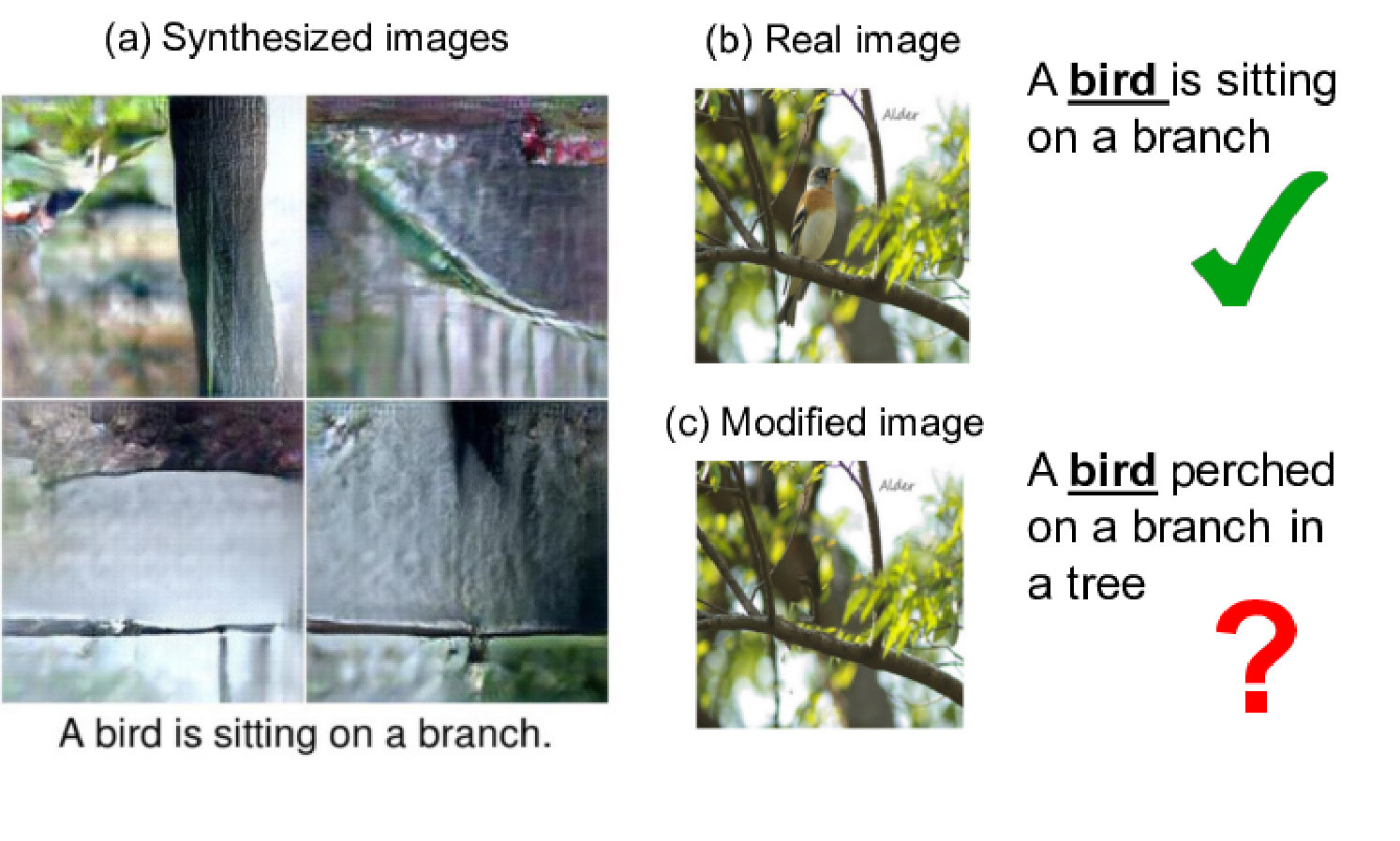 Figure 1
 Figure 2
 Figure 3
 Figure 4
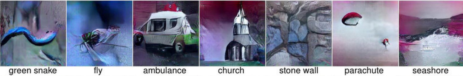 Figure 5
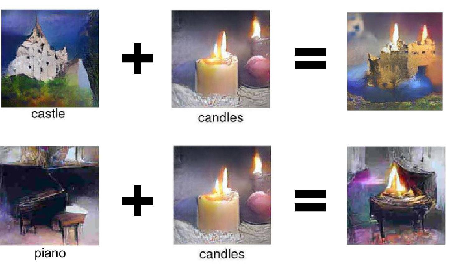 Figure 6
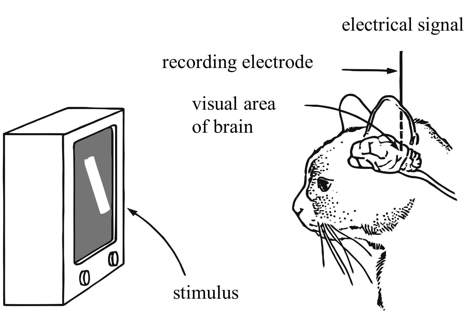 Figure 7
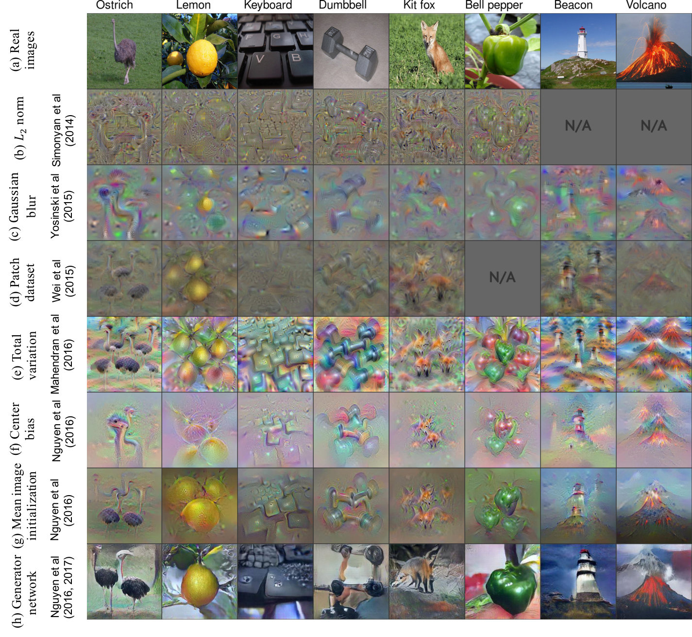 Figure 8
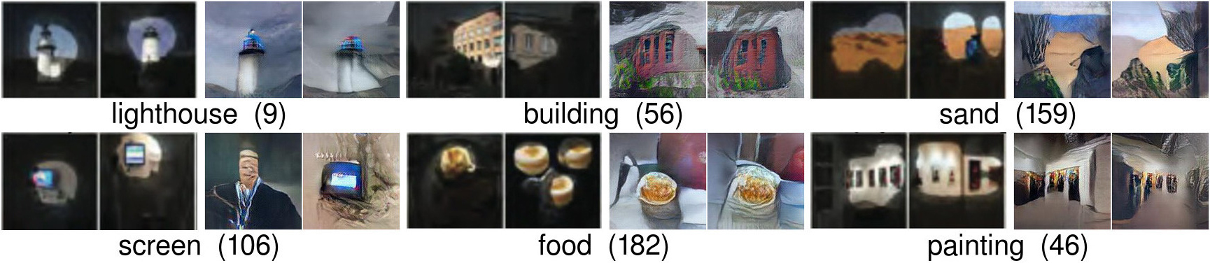 Figure 9
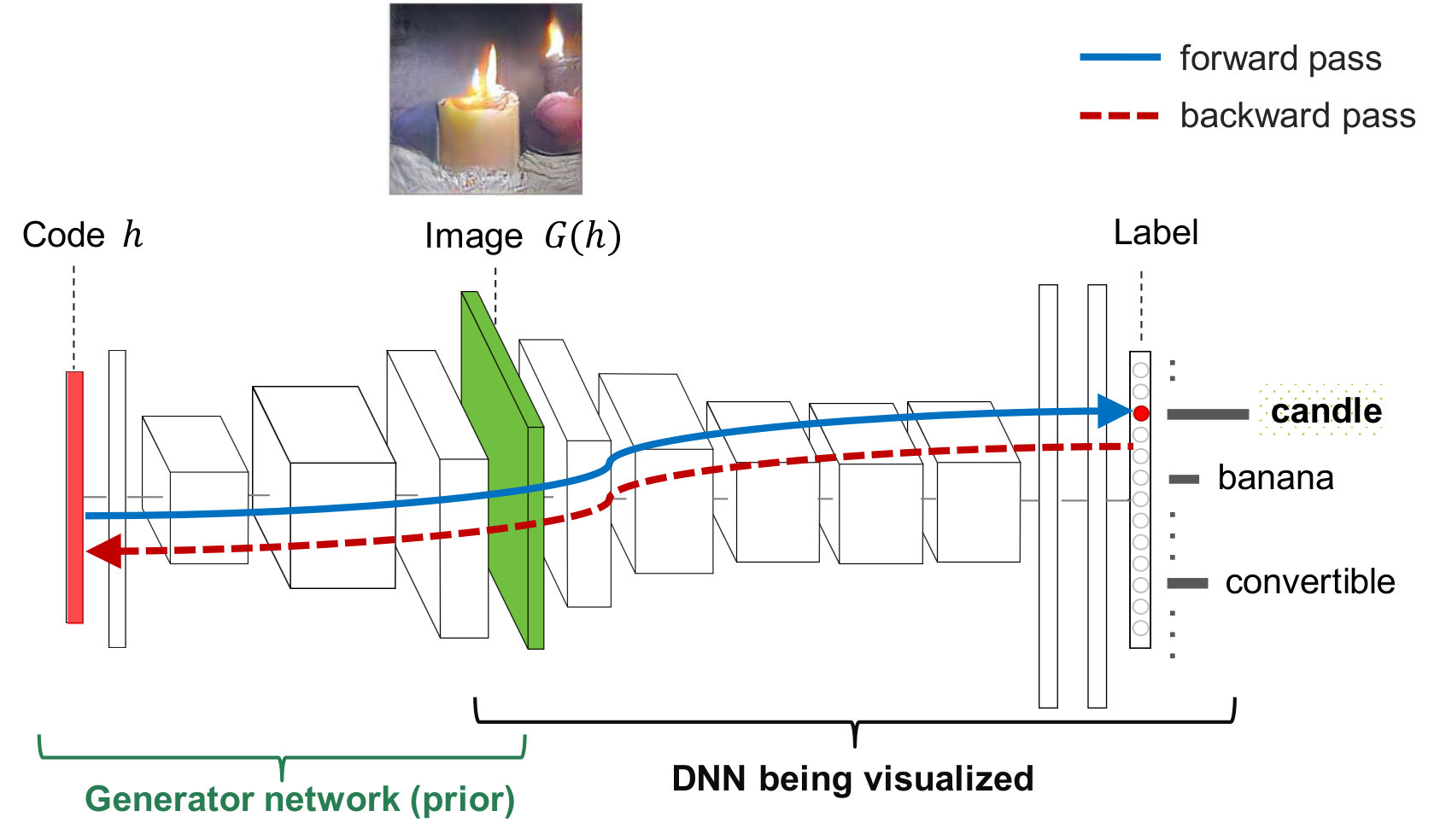 Figure 10
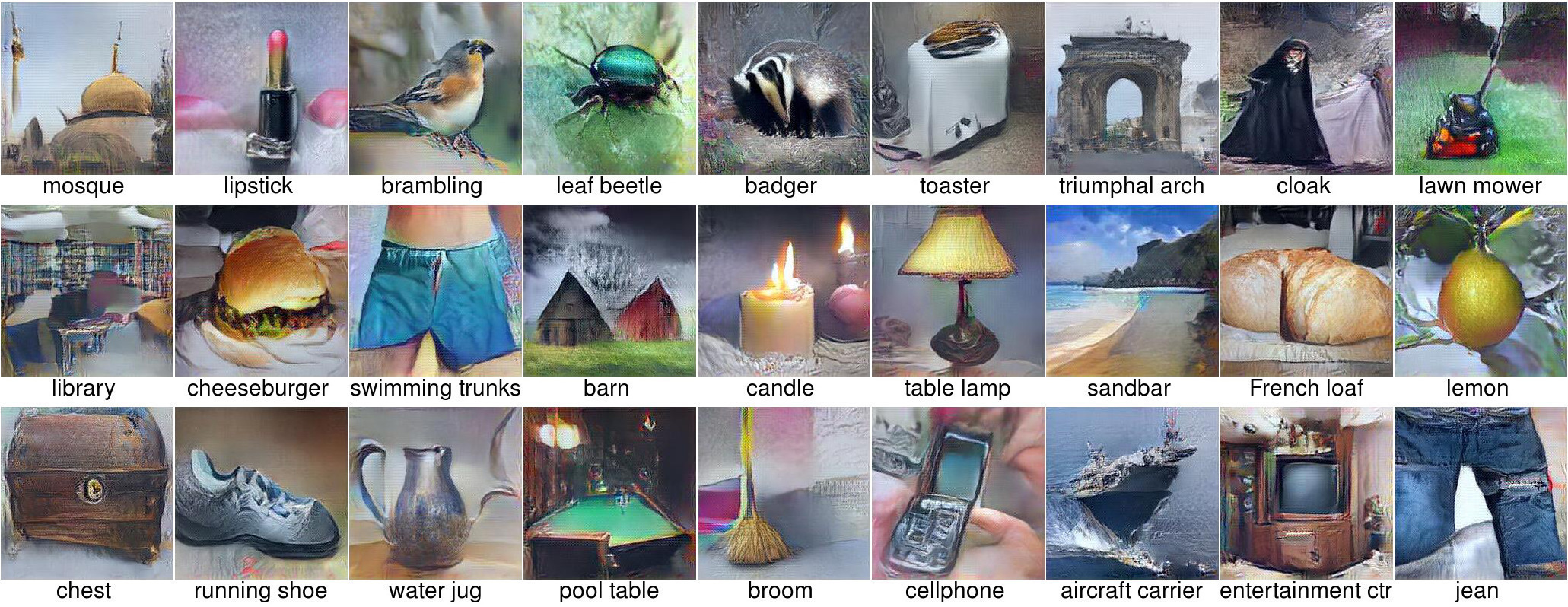 Figure 11
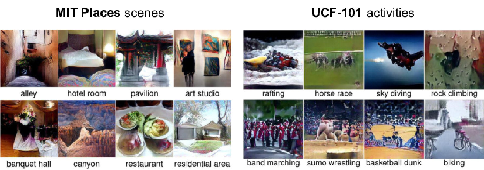 Figure 12
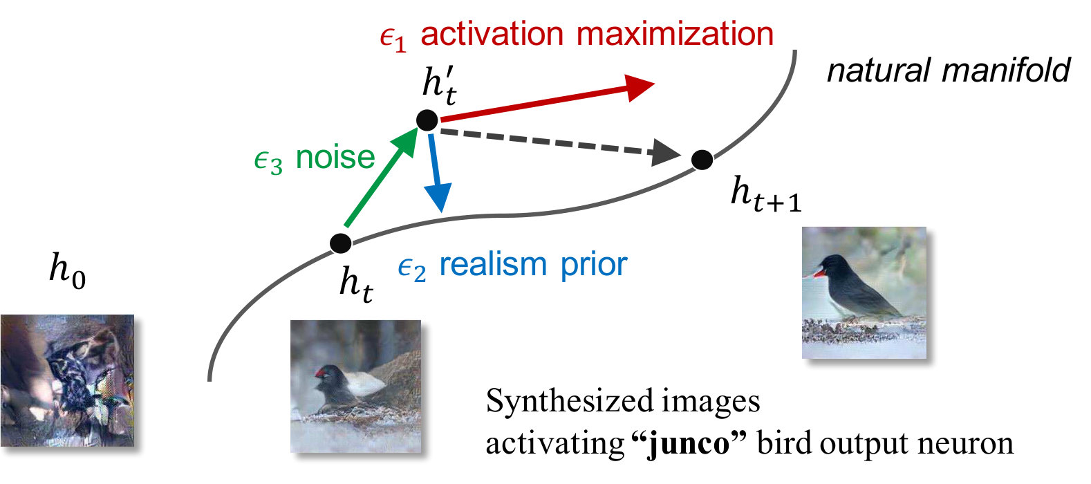 Figure 13
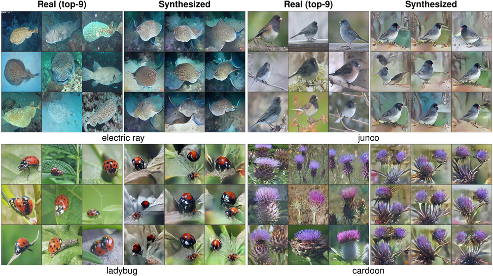 Figure 14
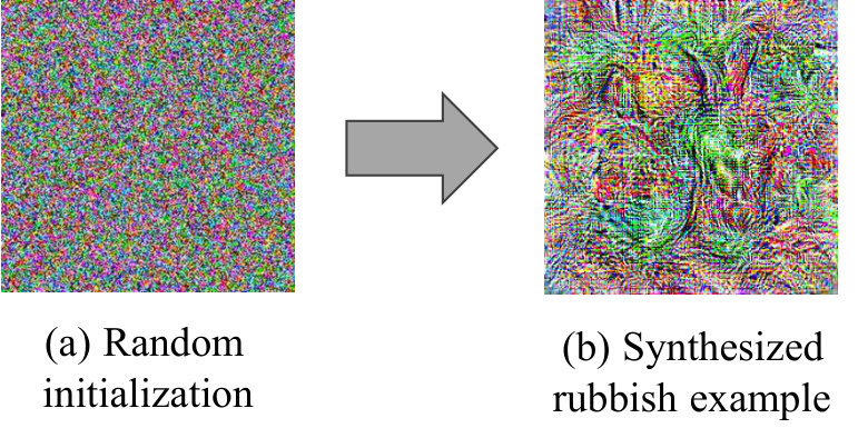 Figure 15
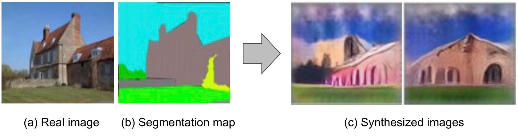 Figure 16
| a. Derivative of raw activations. Worked well in practice [27, 10] but may produce non-selective stimuli and is not quite the right term under the probabilistic framework in Sec. 4.2. | |
|---|---|
| b. Derivative of softmax. Previously avoided due to poor performance [42, 48], but poor performance may have been due to ill-conditioned optimization rather than the inclusion of logits from other classes. | |
| c. Derivative of log of softmax. Correct term under the sampler framework in Sec. 4.2. Well-behaved under optimization, perhaps due to the term untouched by the multiplier. |
Peer Reviews
No public reviews on file for this paper yet. If you reviewed it on a platform where reviews are public (OpenReview, ICLR, NeurIPS, ICML), you can paste yours below so the community can read it here.
Code & Models
Videos
No videos yet. Explain this paper in a talk, walkthrough, or lecture? Add one.
Taxonomy
MethodsAttention Model
lstlistingsection
11institutetext: Auburn University
22institutetext: Uber AI Labs
33institutetext: University of Wyoming
Understanding Neural Networks
via Feature Visualization: A survey
Anh Nguyen 11
Jason Yosinski 22
Jeff Clune 2233 [email protected]
Abstract
A neuroscience method to understanding the brain is to find and study the preferred stimuli that highly activate an individual cell or groups of cells. Recent advances in machine learning enable a family of methods to synthesize preferred stimuli that cause a neuron in an artificial or biological brain to fire strongly. Those methods are known as Activation Maximization (AM) [10] or Feature Visualization via Optimization. In this chapter, we (1) review existing AM techniques in the literature; (2) discuss a probabilistic interpretation for AM; and (3) review the applications of AM in debugging and explaining networks.
Keywords:
N
eural networks, feature visualization, activation maximization, generator network, generative models, optimization
1 Introduction
Understanding the human brain has been a long-standing quest in human history. One path to understanding the brain is to study what each neuron111In this chapter, “neuron”, “cell”, “unit”, and “feature” are used interchangeably. codes for [17], or what information its firing represents. In the classic 1950’s experiment, Hubel and Wiesel studied a cat’s brain by showing the subject different images on a screen while recording the neural firings in the cat’s primary visual cortex (Fig. 1). Among a variety of test images, the researchers found oriented edges to cause high responses in one specific cell [14]. That cell is referred to as an edge detector and such images are called its preferred stimuli. The same technique later enabled scientists to discover fundamental findings of how neurons along the visual pathway detect increasingly complex patterns: from circles, edges to faces and high-level concepts such as one’s grandmother [3] or specific celebrities like the actress Halle Berry [37].
Similarly, in machine learning (ML), visually inspecting the preferred stimuli of a unit can shed more light into what the neuron is doing [49, 48]. An intuitive approach is to find such preferred inputs from an existing, large image collection e.g. the training or test set [49]. However, that method may have undesired properties. First, it requires testing each neuron on a large image set. Second, in such a dataset, many informative images that would activate the unit may not exist because the image space is vast and neural behaviors can be complex [28]. Third, it is often ambiguous which visual features in an image are causing the neuron to fire e.g. if a unit is activated by a picture of a bird on a tree branch, it is unclear if the unit “cares about” the bird or the branch (Fig. 13b). Fourth, it is not trivial how to extract a holistic description of what a neuron is for from the typically large set of stimuli preferred by a neuron.
A common practice is to study the top 9 highest activating images for a unit [48, 49]; however, the top-9 set may reflect only one among many types of features that are preferred by a unit [29].
Instead of finding real images from an existing dataset, one can synthesize the visual stimuli from scratch [32, 10, 27, 25, 42, 46, 29]. The synthesis approach offers multiple advantages: (1) given a strong image prior, one may synthesize (i.e. reconstruct) stimuli without the need to access the target model’s training set, which may not be available in practice (see Sec. 5); (2) more control over the types and contents of images to synthesize, which helps shed light on more controlled research experiments.
Activation Maximization Let be the parameters of a classifier that maps an image (that has color channels, each of which is pixels wide and pixels high) onto a probability distribution over the output classes. Finding an image that maximizes the activation of a neuron indexed in a given layer of the classifier network can be formulated as an optimization problem:
[TABLE]
This problem was introduced as activation maximization222Also sometimes referred to as feature visualization [32, 29, 48]. In this chapter, the phrase “visualize a unit” means “synthesize preferred images for a single neuron”. (AM) by Erhan, Bengio and others [10]. Here, returns the activation value of a single unit as in many previous works [28, 27, 29]; however, it can be extended to return any neural response that we wish to study e.g. activating a group of neurons [24, 33, 26]. The remarkable DeepDream visualizations [24] were created by running AM to activate all the units across a given layer simultaneously. In this chapter, we will write instead of when the exact indices can be omitted for generality.
AM is a non-convex optimization problem for which one can attempt to find a local minimum via gradient-based [44] or non-gradient methods [30]. In post-hoc interpretability [23], we often assume access to the parameters and architecture of the network being studied. In this case, a simple approach is to perform gradient ascent [48, 10, 27, 31] with an update rule such as:
[TABLE]
That is, starting from a random initialization (here, a random image), we iteratively take steps in the input space following the gradient of to find an input that highly activates a given unit. is the step size and is chosen empirically.
Note that this gradient ascent process is similar to the gradient descent process used to train neural networks via backpropagation [39], except that here we are optimizing the network input instead of the network parameters , which are frozen.333Therefore, hereafter, we will write instead of , omitting , for simplicity. We may stop the optimization when the neural activation has reached a desired threshold or a certain number of steps has passed.
In practice, synthesizing an image from scratch to maximize the activation alone (i.e. an unconstrained optimization problem) often yields uninterpretable images [28]. In a high-dimensional image space, we often find rubbish examples (also known as fooling examples [28]) e.g. patterns of high-frequency noise that look like nothing but that highly activate a given unit (Fig. 2).
In a related way, if starting AM optimization from a real image (instead of a random one), we may easily encounter adversarial examples [44] e.g. an image that is slightly different from the starting image (e.g. of a school bus), but that a network would give an entirely different label e.g. “ostrich” [44]. Those early AM visualizations [44, 28] revealed huge security and reliability concerns with machine learning applications and informed a plethora of follow-up adversarial attack and defense research [1, 16].
Networks that we visualize Unless otherwise noted, throughout the chapter, we demonstrate AM on CaffeNet, a specific pre-trained model of the well-known AlexNet convnets [18] to perform single-label image classification on the ILSVRC 2012 ImageNet dataset [7, 40].
2 Activation Maximization via Hand-designed Priors
Examples like those in Fig. 2b are not human-recognizable. While the fact that the network responds strongly to such images is intriguing and has strong implications for security, if we cannot interpret the images, it limits our ability to understand what the unit’s purpose is. Therefore, we want to constrain the search to be within a distribution of images that we can interpret e.g. photo-realistic images or images that look like those in the training set. That can be accomplished by incorporating natural image priors into the objective function, which was found to substantially improve the recognizability of AM images [48, 21, 29, 27, 32]. For example, an image prior may encourage smoothness [21] or penalize pixels of extreme intensity [42]. Such constraints are often incorporated into the AM formulation as a regularization term :
[TABLE]
For example, to encourage the smoothness in AM images, may compute the total variation (TV) across an image [21]. That is, in each update, we follow the gradients to (1) maximize the neural activation; and (2) minimize the total variation loss:
[TABLE]
However, in practice, we do not always compute the analytical gradient . Instead, we may define a regularization operator (e.g. a Gaussian blur kernel), and map to a more regularized (e.g. slightly blurrier as in [48]) version of itself in every step. In this case, the update step becomes:
[TABLE]
Note that this update form in Eq. 5 is strictly more expressive [48], and allows the use of non-differentiable regularizers .
Local statistics AM images without priors often appear to have high-frequency patterns and unnatural colors (Fig. 2b). Many regularizers have been designed in the literature to ameliorate these problems including:
- •
Penalize extreme-intensity pixels via -norm [42, 48, 46] (Fig. 3b).
- •
Penalize high-frequency noise (i.e. smoothing) via total variation [21, 29] (Fig. 3e), Gaussian blurring [48, 54] (Fig. 3c) or a bilateral filter [45].
- •
Randomly jitter, rotate, or scale the image before each update step to synthesize stimuli that are robust to transformations, which has been shown to make images clearer and more interpretable [32, 24].
- •
Penalize the high frequencies in the gradient image (instead of the visualization ) via Gaussian blurring [54, 32].
- •
Encourage patch-level color statistics to be more realistic by (1) matching those of real images from a dataset [46] (Fig. 3d) or (2) learning a Gaussian mixture model of real patches [24].
While substantially improving the interpretability of images (compared to high-frequency rubbish examples), these methods only effectively attempt to match the local statistics of natural images.
Global structures Many AM images still lack global coherence; for example, an image synthesized to highly activate the “bell pepper” output neuron (Fig. 3b–e) may exhibit multiple bell-pepper segments scattered around the same image rather than a single bell pepper. Such stimuli suggest that the network has learned some local discriminative features e.g. the shiny, green skin of bell peppers, which are useful for the classification task. However, it raises an interesting question: Did the network ever learn the global structures (e.g. the whole pepper) or only the local discriminative parts? The high-frequency patterns as in Fig. 3b–e might also be a consequence of optimization in the image space. That is, when making pixel-wise changes, it is non-trivial to ensure global coherence across the entire image. Instead, it is easy to increase neural activations by simply creating more local discriminative features in the stimulus.
Previous attempts to improve the global coherence include:
- •
Gradually paint the image by scaling it and alternatively following the gradients from multiple output layers of the network [54].
- •
Bias the image changes to be near the image center [29] (Fig. 3g).
- •
Initialize optimization from an average image (computed from real training set images) instead of a random one [29] (Fig. 3h).
While these methods somewhat improved the global coherence of images (Fig. 3g–h), they rely on a variety of heuristics and introduce extra hyperparameters [54, 29]. In addition, there is still a large realism gap between the real images and these visualizations (Fig. 3a vs. h).
Diversity A neuron can be multifaceted in that it responds strongly to multiple distinct types of stimuli, i.e. facets [29]. That is, higher-level features are more invariant to changes in the input [49, 19]. For example, a face-detecting unit in CaffeNet [18] was found to respond to both human and lion faces [48]. Therefore, we wish to uncover different facets via AM in order to have a fuller understanding of a unit.
However, AM optimization starting from different random images often converge to similar results [10, 29]—a phenomenon also observed when training neural networks with different initializations [20]. Researchers have proposed different techniques to improve image diversity such as:
- •
Drop out certain neural paths in the network when performing backpropagation to produce different facets [46].
- •
Cluster the training set images into groups, and initialize from an average image computed from each group’s images [29].
- •
Maximize the distance (e.g. cosine similarity in the pixel space) between a reference image and the one being synthesized [32].
- •
Activate two neurons at the same time e.g. activating (bird + apron) and (bird + candles) units would produce two distinct images of birds that activate the same bird unit [27] (Fig. 10).
- •
Add noise to the image in every update to increase image diversity [26].
While obtaining limited success, these methods also introduce extra hyperparameters and require further investigation. For example, if we enforce two stimuli to be different, exactly how far should they be and in which similarity metric should the difference be measured?
3 Activation Maximization via Deep Generator Networks
Much previous AM research were optimizing the preferred stimuli directly in the high-dimensional image space where pixel-wise changes are often slow and uncorrelated, yielding high-frequency visualizations (Fig. 3b–e). Instead, Nguyen et al. [27] propose to optimize in the low-dimensional latent space of a deep generator network, which they call Deep Generator Network Activation Maximization (DGN-AM). They train an image generator network to take in a highly compressed code and output a synthetic image that looks as close to real images from the ImageNet dataset [40] as possible. To produce an AM image for a given neuron, the authors optimize in the input latent space of the generator so that it outputs an image that activates the unit of interest (Fig. 4). Intuitively, DGN-AM restricts the search to only the set of images that can be drawn by the prior and encourages the image updates to be more coherent and correlated compared to pixel-wise changes (where each pixel is modified independently).
Generator networks We denote the sub-network of CaffeNet [18] that maps images onto 4096-D features as an encoder . We train a generator network to invert i.e. . In addition to the reconstruction losses, the generator was trained using the Generative Adversarial Network (GAN) loss [13] to improve the image realism. More training details are in [27, 9]. Intuitively, can be viewed as an artificial general “painter” that is capable of painting a variety of different types of images, given an arbitrary input description (i.e. a latent code or a condition vector). The idea is that would be able to faithfully portray what a target network has learned, which may be recognizable or unrecognizable patterns to humans.
Optimizing in the latent space Intuitively, we search in the input code space of the generator to find a code such that the image maximizes the neural activation (see Fig. 4). The AM problem in Eq. 3 now becomes:
[TABLE]
That is, we take steps in the latent space following the below update rule:
[TABLE]
Note that, here, the regularization term is on the latent code instead of the image . Nguyen et al. [27] implemented a small amount of regularization and also clipped the code. These hand-designed regularizers can be replaced by a strong, learned prior for the code [26].
Optimizing in the latent space of a deep generator network showed a great improvement in image quality compared to previous methods that optimize in the pixel space (Fig. 5; and Fig. 3b–h vs. Fig. 3i). However, images synthesized by DGN-AM have limited diversity—they are qualitatively similar to the real top-9 validation images that highest activate a given unit (Fig. 6).
To improve the image diversity, Nguyen et al. [26] harnessed a learned realism prior for via a denoising autoencoder (DAE), and added a small amount of Gaussian noise in every update step to improve image diversity [26]. In addition to an improvement in image diversity, this AM procedure also has a theoretical probabilistic justification, which is discussed in Section 4.
4 Probabilistic interpretation for Activation Maximization
In this section, we first make a note about the AM objective, and discuss a probabilistically interpretable formulation for AM, which is first proposed in Plug and Play Generative Networks (PPGNs) [26], and then interpret other AM methods under this framework. Intuitively, the AM process can be viewed as sampling from a generative model, which is composed of (1) an image prior and (2) a recognition network that we want to visualize.
4.1 Synthesizing selective stimuli
We start with a discussion on AM objectives. In the original AM formulation (Eq. 1), we only explicitly maximize the activation of a unit indexed in layer ; however, in practice, this objective may surprisingly also increase the activations of some other units in the same layer and even higher than [27]. For example, maximizing the output activation for the “hartebeest” class is likely to yield an image that also strongly activates the “impala” unit because these two animals are visually similar [27]. As the result, there is no guarantee that the target unit will be the highest activated across a layer. In that case, the resultant visualization may not portray what is unique about the target unit .
Instead, we are interested in selective stimuli that highly activate only , but not . That is, we wish to maximize such that it is the highest single activation across the same layer . To enforce that selectivity, we can either maximize the softmax or log of softmax of the raw activations across a layer [42, 26] where the softmax transformation for unit across layer is given as . Such selective stimuli (1) are more interpretable and preferred in neuroscience [3] because they contain only visual features exclusively for one unit of interest but not others; (2) naturally fit in our probabilistic interpretation discussed below.
4.2 Probabilistic framework
Let us assume a joint probability distribution where denotes images, and is a categorical variable for a given neuron indexed in layer . This model can be decomposed into an image density model and an image classifier model:
[TABLE]
Note that, when is the output layer of an ImageNet 1000-way classifier [18], also represents the image category (e.g. “volcano”), and is the classification probability distribution (often modeled via softmax).
We can construct a Metropolis-adjusted Langevin [38] (MALA) sampler for our model [26]. This variant of MALA [26] does not have the accept/reject step, and uses the following transition operator:444We abuse notation slightly in the interest of space and denote as a sample from that distribution. The first step size is given as in anticipation of later splitting into separate and terms.
[TABLE]
Since is a categorical variable, and chosen to be a fixed neuron outside the sampler, the above update rule can be re-written as:
[TABLE]
Decoupling into explicit and multipliers, and expanding the into explicit partial derivatives, we arrive at the following update rule:
[TABLE]
An intuitive interpretation of the roles of these three terms is illustrated in Fig. 7 and described as follows:
- •
term: take a step toward an image that causes the neuron to be the highest activated across a layer (Fig. 7; red arrow)
- •
term: take a step toward a generic, realistic-looking image (Fig. 7; blue arrow).
- •
term: add a small amount of noise to jump around the search space to encourage image diversity (Fig. 7; green arrow).
Maximizing raw activations vs. softmax Note that the term in Eq. 11 is not the same as the gradient of raw activation term in Eq. 2. We summarize in Table 4.2 three variants of computing this gradient term: (1) derivative of logits; (2) derivative of softmax; and (3) derivative of log of softmax. Several previous works empirically reported that maximizing raw, pre-softmax activations produces better visualizations than directly maximizing the softmax values (Table 4.2a vs. b); however, this observation had not been fully justified [42]. Nguyen et al. [26] found the log of softmax gradient term (1) working well empirically; and (2) theoretically justifiable under the probabilistic framework in Section 4.2.
The reference list from the paper itself. Each links out to its DOI / PubMed record.
- 1[1] Akhtar, N., Mian, A.: Threat of adversarial attacks on deep learning in computer vision: A survey. IEEE Access 6, 14410–14430 (2018)
- 2[2] Alcorn, M.A., Li, Q., Gong, Z., Wang, C., Mai, L., Ku, W.S., Nguyen, A.: Strike (with) a pose: Neural networks are easily fooled by strange poses of familiar objects. In: Proceedings of the IEEE Conference on Computer Vision and Pattern Recognition. vol. 1, p. 4. IEEE (2019)
- 3[3] Baer, M., Connors, B.W., Paradiso, M.A.: Neuroscience: Exploring the brain (2007)
- 4[4] Bau, D., Zhou, B., Khosla, A., Oliva, A., Torralba, A.: Network dissection: Quantifying interpretability of deep visual representations. In: Computer Vision and Pattern Recognition (CVPR), 2017 IEEE Conference on. pp. 3319–3327. IEEE (2017)
- 5[5] Bengio, Y., Mesnil, G., Dauphin, Y., Rifai, S.: Better mixing via deep representations. In: International Conference on Machine Learning. pp. 552–560 (2013)
- 6[6] Brock, A., Lim, T., Ritchie, J.M., Weston, N.: Neural photo editing with introspective adversarial networks. ar Xiv preprint ar Xiv:1609.07093 (2016)
- 7[7] Deng, J., et al.: Imagenet: A large-scale hierarchical image database. In: CVPR (2009)
- 8[8] Donahue, J., Hendricks, L.A., Guadarrama, S., Rohrbach, M., et al.: Long-term recurrent convolutional networks for visual recognition and description. In: Computer Vision and Pattern Recognition (2015)
