Excitation of interfacial waves via near---resonant surface---interfacial wave interactions
Joseph Zaleski, Philip Zaleski, Yuri V Lvov

TL;DR
This paper develops a Hamiltonian-based formalism to analyze resonant interactions between surface and interfacial waves in a two-layer system, revealing energy transfer mechanisms influenced by wind and wave spectra.
Contribution
It introduces a novel Hamiltonian framework for coupled surface-interfacial wave interactions, including spectral energy transfer and growth rate calculations.
Findings
Energy transfer from surface to interfacial waves can occur over hours.
Most effective energy transfer at wind speeds near sea capping.
Interfacial waves can be generated oblique to wind direction.
Abstract
We consider interactions between surface and interfacial waves in the two layer system. Our approach is based on the Hamiltonian structure of the equations of motion, and includes the general procedure for diagonalization of the quadratic part of the Hamiltonian. Such diagonalization allows us to derive the interaction crossection between surface and interfacial waves and to derive the coupled kinetic equations describing spectral energy transfers in this system. Our kinetic equation allows resonant and near resonant interactions. We find that the energy transfers are dominated by the class III resonances of \cite{Alam}. We apply our formalism to calculate the rate of growth for interfacial waves for different values of the wind velocity. Using our kinetic equation, we also consider the energy transfer from the wind generated surface waves to interfacial waves for the case when the…
Click any figure to enlarge with its caption.
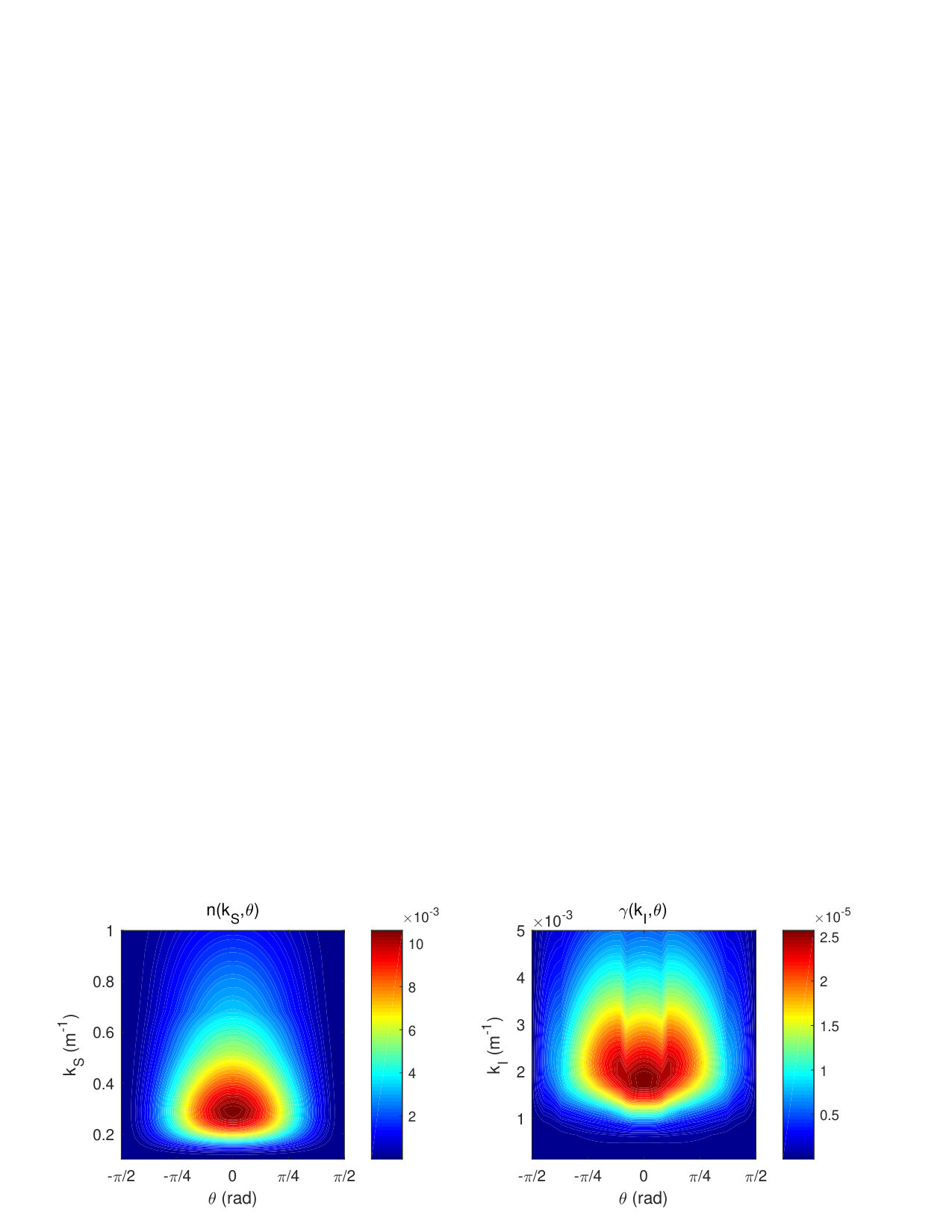 Figure 1
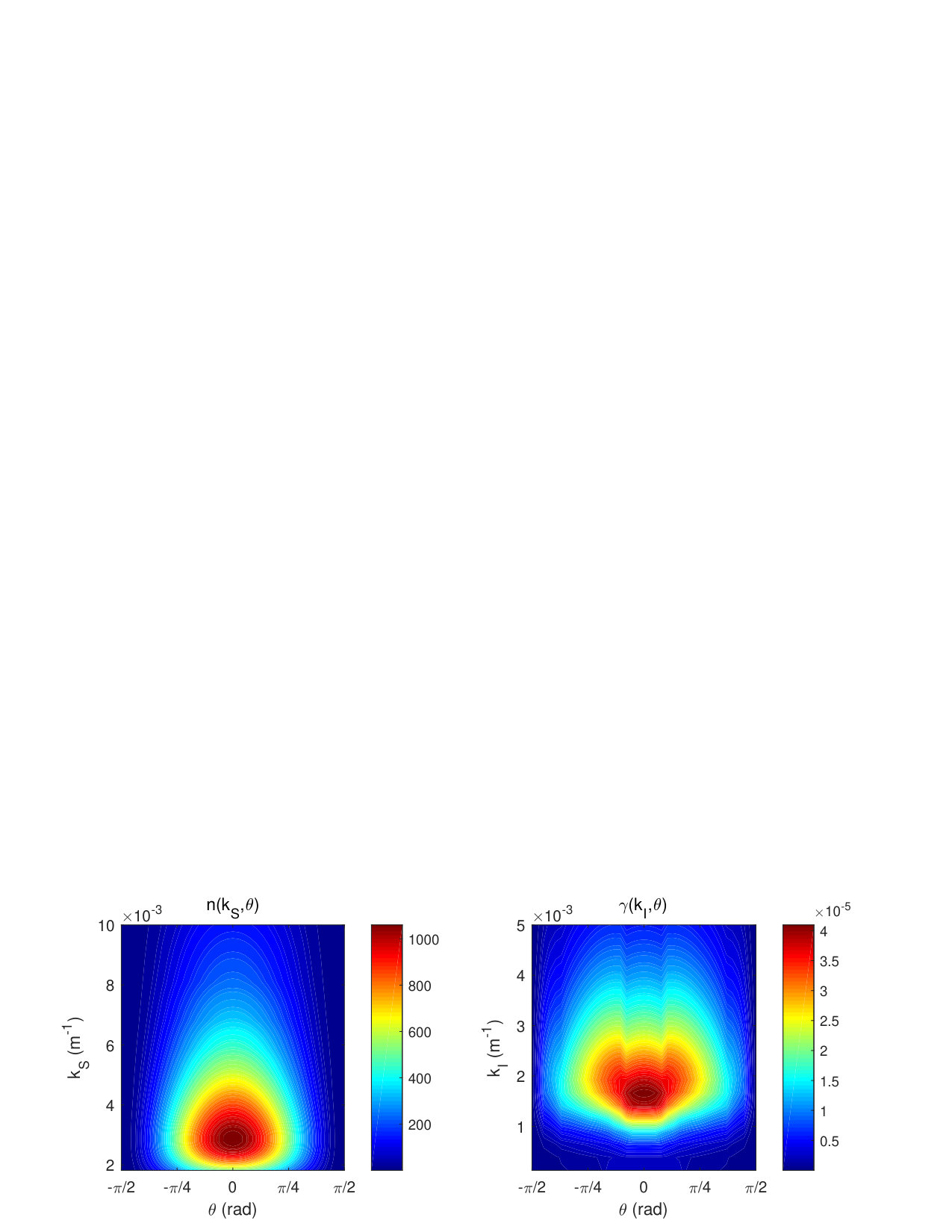 Figure 2
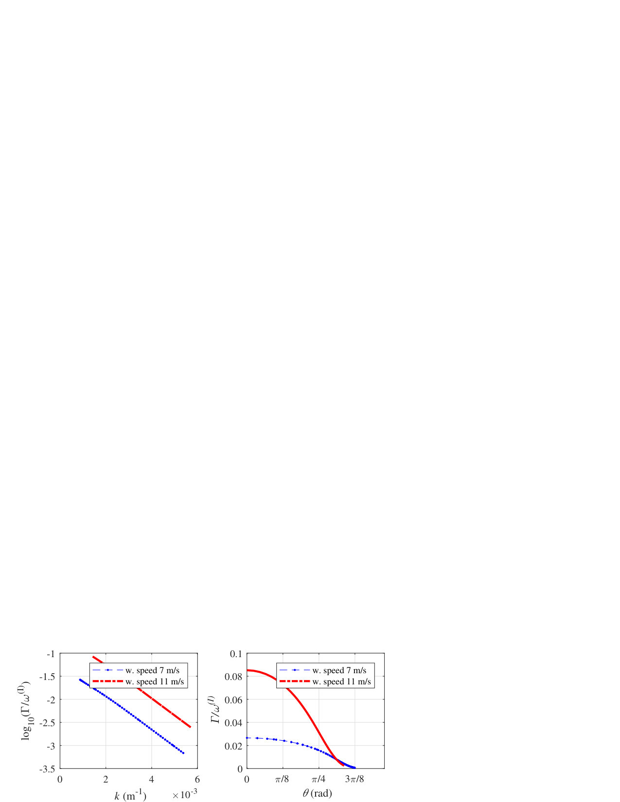 Figure 3
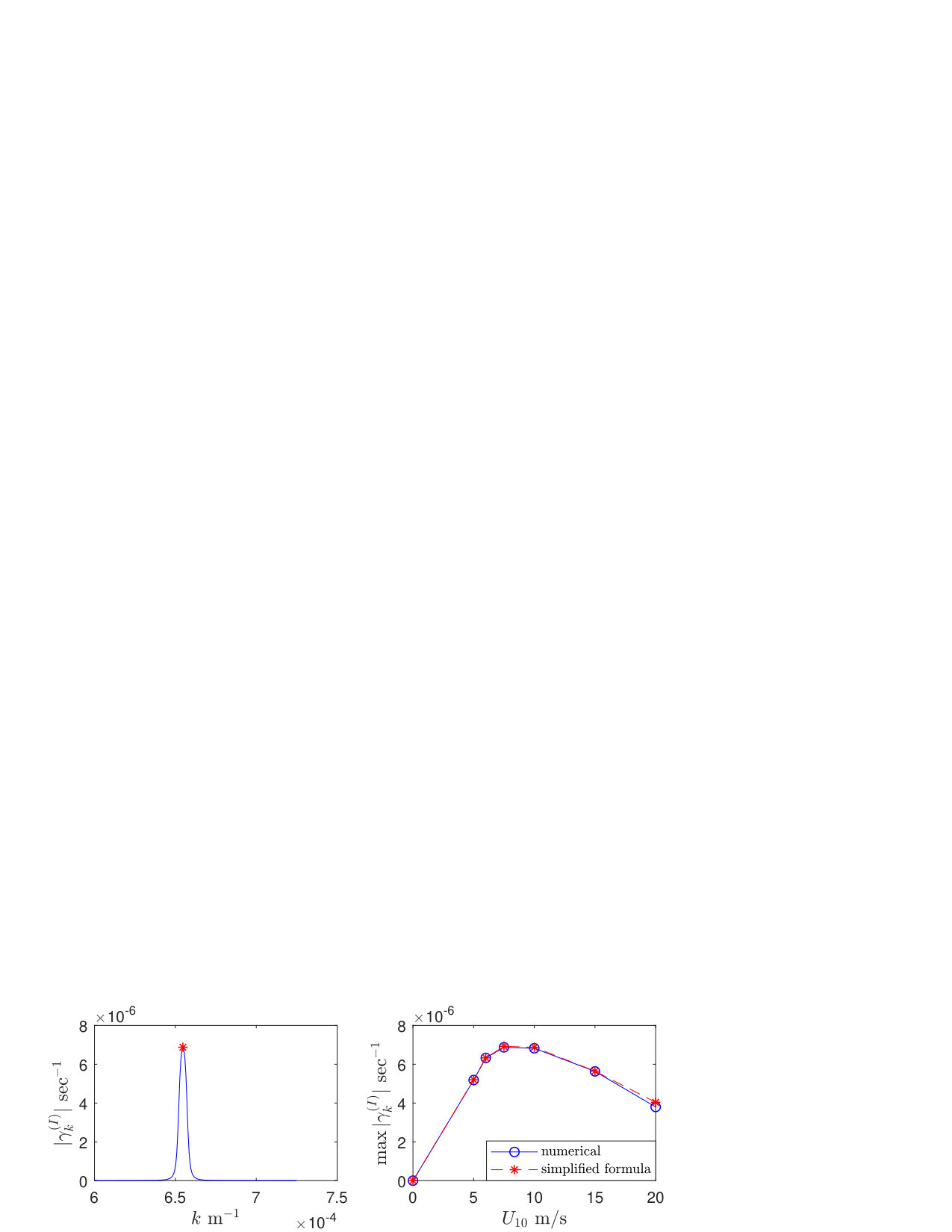 Figure 4
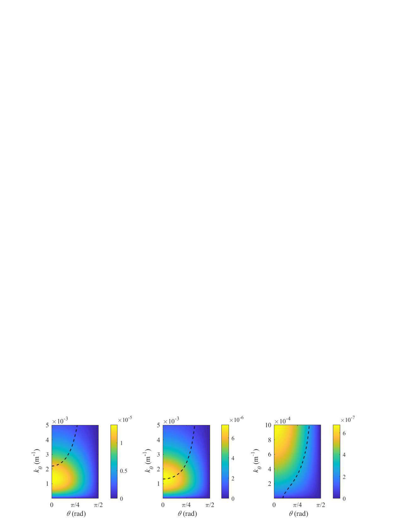 Figure 5
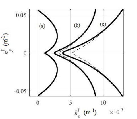 Figure 6
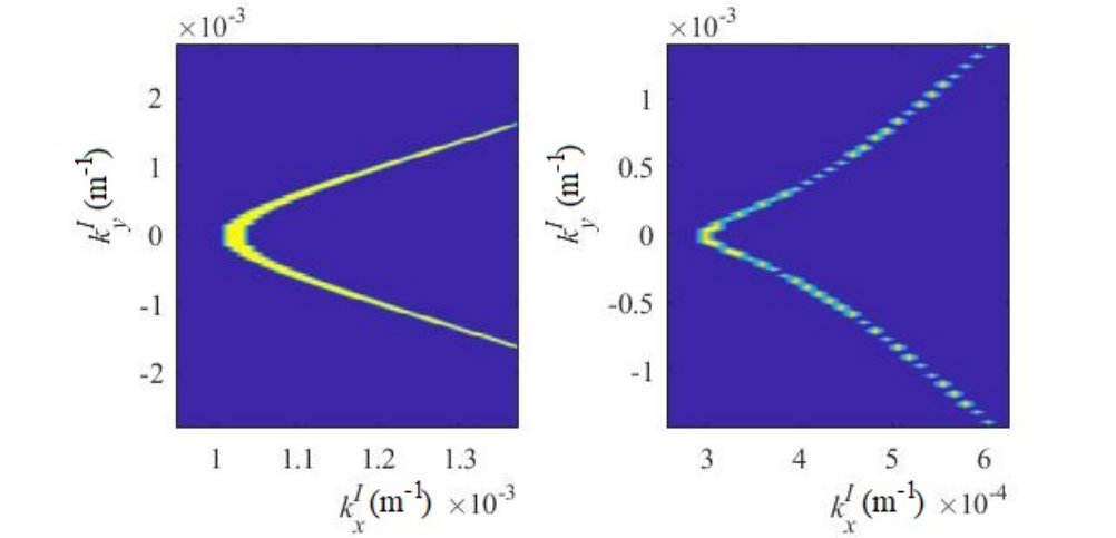 Figure 7
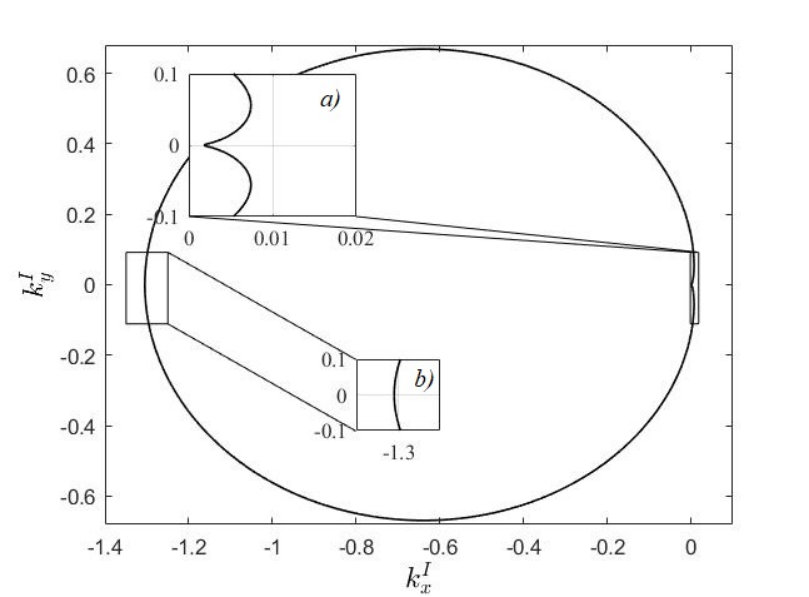 Figure 8
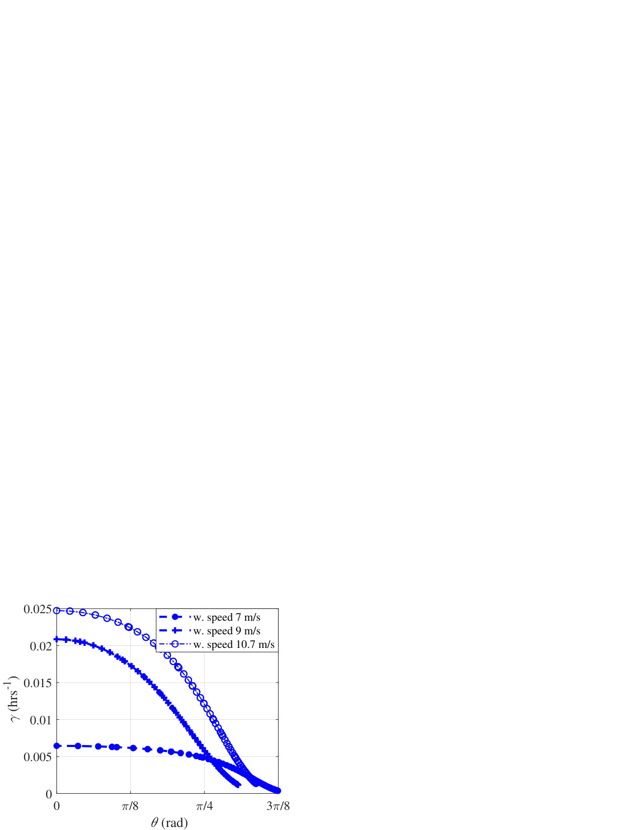 Figure 9
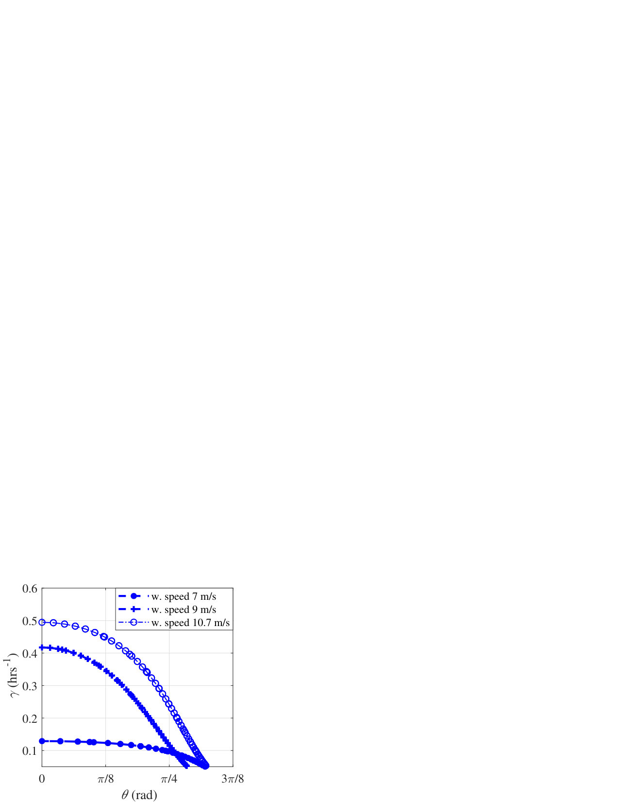 Figure 10
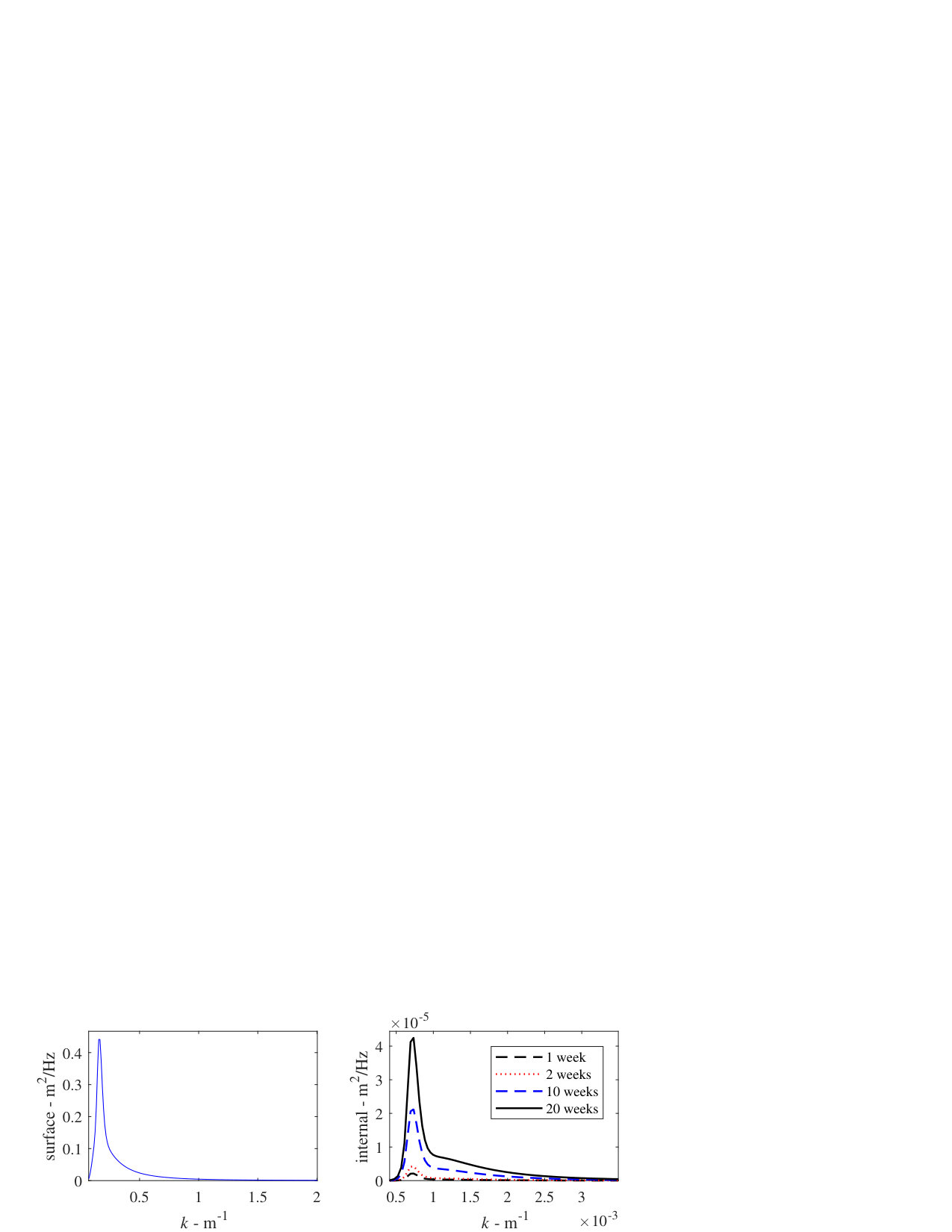 Figure 11
Peer Reviews
No public reviews on file for this paper yet. If you reviewed it on a platform where reviews are public (OpenReview, ICLR, NeurIPS, ICML), you can paste yours below so the community can read it here.
Videos
No videos yet. Explain this paper in a talk, walkthrough, or lecture? Add one.
Taxonomy
TopicsOcean Waves and Remote Sensing · Coastal and Marine Dynamics · Oceanographic and Atmospheric Processes
Excitation of interfacial waves via surface—interfacial wave interactions
Joseph Zaleski \aff1
Philip Zaleski \aff2
Yuri V. Lvov \aff1 \corresp
\aff1Department of Mathematics, Rensselaer Polytechnic Institute, NY 12180, USA \aff2Department of Mathematics, New Jersey Institute of Technology, Newark, NJ 07102, USA
Abstract
We consider interactions between surface and interfacial waves in the two layer system. Our approach is based on the Hamiltonian structure of the equations of motion, and includes the general procedure for diagonalization of the quadratic part of the Hamiltonian. Such diagonalization allows us to derive the interaction crossection between surface and interfacial waves and to derive the coupled kinetic equations describing spectral energy transfers in this system. Our kinetic equation allows resonant and near resonant interactions. We find that the energy transfers are dominated by the class III resonances of Alam (2012). We apply our formalism to calculate the rate of growth for interfacial waves for different values of the wind velocity. Using our kinetic equation, we also consider the energy transfer from the wind generated surface waves to interfacial waves for the case when the spectrum of the surface waves is given by the JONSWAP spectrum and interfacial waves are initially absent. We find that such energy transfer can occur along a timescale of hours; there is a range of wind speeds for the most effective energy transfer at approximately the wind speed corresponding to white capping of the sea. Furthermore, interfacial waves oblique to the direction of the wind are also generated.
keywords:
1 Introduction
1.1 Background
The term “ocean waves” typically evokes images of surface waves shaking ships during storms in the open ocean, or breaking rhythmically near the shore. However, much of the ocean wave action takes place far underneath the surface, and consists of surfaces of constant density being disturbed and modulated.
When wind blows over the ocean, it excites surface waves. These surface waves in turn excite the internal waves. Therefore the coupling between surface and interfacial waves provide a key mechanism of coupling an atmosphere and the ocean. The simplest conceptual model describing such interaction is a two layer model figure (1), with the lighter fluid with free surface being on top of the heavier fluid with the rigid bottom. This two layer model has been actively studied in the last few decades from the angle of weakly nonlinear resonant interactions between surface and interfacial layers Ball (1964); Thorpe (1966); Gargettt & Hughes (1972); Watson et al. (1976); Olbers & Herterich (1979); Segur (1980); Dysthe & Das (1981); Watson (1989, 1994); Alam (2012); Tanaka & Wakayama (2015); Constantin & Ivanov (2015); Olbers & Eden (2016).
The strength of such nonlinear interactions has been the subject of long debate. Earlier approaches include the calculations of Thorpe (1966); Olbers & Herterich (1979). Most recently, Olbers & Eden (2016) found the annual mean energy flux integrated globally over the oceans to be about terawatts.
Ball (1964) showed the existence of a closed curve of triad resonances for two dimensional wave vectors corresponding to interactions between waves of all possible orientations. He emphasized the cases in which two counter propagating surface waves drive an interfacial wave, and two counter propagating interfacial waves drive a surface wave. Later, these classes of resonances were referred to as class I and class II interactions. In class I, two surface waves counter propagate with roughly equal wavelength, with the interfacial wave having shorter wavelength. In class II, the interfacial waves counter propagate with the surface wave having roughly twice the frequency of the interfacial waves Alam (2012).
Chow (1983) analyzed class I resonances for a two layer model under the assumptions that the bottom layer is of infinite depth and the top layer is shallow. These assumptions allowed to formulate the triad resonance condition in a more general way, namely that the group speed of a surface wave envelope matches the phase speed of the interfacial wave. Using this condition, Chow derived evolution equations for a surface wave train coupled to interfacial waves. He found a band of wavenumbers that are unstable, thus facilitating energy transfer from the surface waves to the interfacial waves. However, he found that the energy transfer rate was smaller than the transfer rate for resonant triad interactions.
Watson (1989) considered surface-interfacial waves interaction, taking into account both surface wave dissipation, and broadening of the three wave resonances, using WKB theory.
Alam (2012) considered resonances in the one-dimensional case with collinear waves. He discovered what is now called class III resonances, where the wavelength of the resonant interfacial wave is much longer than that of the two co-propagating surface waves, making it physically relevant in describing the formation of long interfacial waves. Alam showed that these resonances cause a cascade of resonant and near-resonant interactions between surface and interfacial waves and thus could be a viable energy exchange mechanism. He also obtained expressions for the amplitude growth of an interfacial wave in a system with a large number of interacting waves.
Tanaka & Wakayama (2015) considered the two layer system and modeled numerically the primitive equations of motion in 2+1 dimensions (horizontal and vertical direction and time) for the case of a surface wave spectrum based on the Pierson—Moskowitz spectrum Pierson & Moskowitz (1964). Tanaka & Wakayama (2015) showed that the initially still interface experiences excitation with a flux of energy towards smaller wave numbers. For the case of large difference in density between layers, they noticed that the shape of the surface spectrum changes significantly. They noted that this cannot be explained by resonant wave interaction theory because resonant wave interaction theory predicts the existence of the critical surface wave number, below which there could not be any interactions. Consequently, there is a need of a theory not limited to only resonant, but also near resonant interactions.
Olbers & Eden (2016) used an analytical framework that directly derives the flux of energy radiating downward from the mixed layer base with a goal of providing a global map of the energy transfer to the interfacial wave field. They concluded that spontaneous wave generation, where two surface waves create an interfacial wave, becomes dominant over modulational interactions where a preexisting interfacial wave is modulated by a surface wave for wind speeds above 10-15 m/s.
1.2 Overview of the paper
In this paper we derive from first principle wave turbulence theory for wave-wave interactions in the two-layer model. Our theory is based on the recently derived Hamiltonian structure for this system Choi (2019). We derive the kinetic equations describing weakly nonlinear energy transfers between waves. The theory includes both resonant and near-resonant wave-wave interactions, and allows to quantitatively describe coupling between the atmosphere and the ocean.
The paper is written as follows: in section 2 we discuss the governing equations of motion and Hamiltonian structure derived by Choi (2019) for the case of 3+1 dimensions. Notably, the Hamiltonian is expressed explicitly in terms of the interface variables, forming the base needed for our analysis.
In section 3 we derive a canonical transformation to diagonalize the quadratic part of the Hamiltonian to obtain the normal modes. Such a diagonalization reduces the system to an ensemble of waves which are free to the leading order, thus making it amendable to Wave Turbulence theory as described in Zakharov et al. (1992); Nazarenko (2011).
In section 4 we apply Wave Turbulence theory to obtain the system of kinetic equations governing the time evolution of the wave action spectrum of waves (“number of waves”). Furthermore, we calculate the exact matrix elements (interaction crossections) governing such interactions. Our calculations are valid both on and near the resonant–manifold.
In section 5 we test our theory by considering the model problem with the surface described by a single plain wave with frequency being the peak frequency of the JONSWAP spectrum Hassleman et al. (1973). We obtain the Boltzmann rates and corresponding timescales of amplitude growth for excited interfacial waves. The frequencies of the excited interfacial waves are well within the experimental measurements given in buoyancy profiles of the ocean. Furthermore, we generalize the results in Alam (2012) by considering the general case where all wave vectors are two dimensional and not necessarily collinear. Notably, for conditions of long surface swell waves, the dominant interactions occur between surface and interfacial waves which are oblique, a case also noted by Haney & Young (2017). Inspired by Tanaka & Wakayama (2015), we also simulate the evolving spectra for the case when the surface is the 1-D JONSWAP spectrum and the interface is initially at rest.
In section 6 we conclude by summarizing our results and discussing future work.
2 Governing equations
2.1 Equations in physical space
We use a Cartesian coordinate system , with the -plane being the mean free surface and the -axis being directed upward. We consider a two-layer model with the free surface on top and the interface between the layers. We denote the respective depths of the upper and lower layers by and their densities by , , with the difference in density between layers to be , where subscript “u” refers to the upper and subscript “l” to lower layers. We assume the fluid is homogeneous, incompressible, immersible, inviscid, and irrotational in both layers.
To derive the closed set of coupled equations for the surface velocity potential and displacement and interfacial velocity potential and displacement we start from the Euler equations, incompressibility condition, and kinematic boundary conditions for velocity and pressure continuity along the surface/interface. We then introduce a nonlinearity parameter , the slope of the waves, and make a formal assumption that . This allows us to iterate the resulting equations for a solution representing a wavetrain with wave number . This procedure was recently executed in Choi (2019), and leads to the following system of equations, truncated at the second order of nonlinearity parameter,
[TABLE]
with the nonlocal linear operators and , whose Fourier kernels are given in Appendix (A).
2.2 Hamiltonian
We use the Fourier transformations of the interface variables for the two layer system depicted in figure (1)
[TABLE]
The equations of motion (1) can then be represented by canonically conjugated Hamilton’s equations for the Hamiltonian , given by Choi (2019)
[TABLE]
This is a generalization for two layers of the Hamiltonian formulation described in Zakharov (1968) for surface waves. Here the Hamiltonian, , is a sum of a quadratic Hamiltonian, describing linear noninteracting waves, and a cubic Hamiltonian, describing wave–wave interactions, , where
[TABLE]
where the coupling coefficients are given in Appendix (B). Here denotes the wavenumber and we use the notation that subscripts represent vector arguments, i.e. .
This Hamiltonian is expressed explicitly in terms of the variables at the surfaces of the fluids, and is a significant step forward over the Hamiltonian structure of the two layer system derived in Ambrosi (2000), where the implicit form of the Hamiltonian was obtained.
The Hamiltonian provides the firm theoretical foundation to develop the theory of weak nonlinear interactions of surface and interfacial waves. However to describe the time evolution of the spectral energy density of the waves, the quadratic part of the Hamiltonian of the system (LABEL:H2) needs to be diagonalized, so that the linear part of equations of motion corresponds to distinct noninteracting linear waves. In other words, we need to calculate the normal modes of the system. This task is done in the next section.
3 Canonical transformation to normal modes
In this paper we use the wave turbulence formalism Benney & Newell (1969); Newell (1968); Benney & P.Saffmann (1966); Kadomtsev (1965); Zakharov et al. (1992); Nazarenko (2011) to derive the coupled set of kinetic equations, describing the spectral energy transfers in the coupled system of surface and interfacial waves. First we need to diagonalize the Hamiltonian equations of motion in wave action variables so that waves are free to the leading order. This is done via two canonical transformations; the first being a transformation from interface variables to complex action density variables done in subsection (3.1), the second being a transformation to diagonalize the quadratic Hamiltonian, giving waves which are free to the leading order, performed in Section (3.2). The final form of the Hamiltonian in terms of the normal modes is also derived in subsection (3.2).
3.1 Transformation to complex field variable
We start from the surface variables for the Fourier image of displacement of the upper and lower layers and the Fourier image of the velocity potential on upper and lower surfaces , where denotes the layer, with being the upper, and being the lower layers. We then perform a canonical transformation to complex action variables describing the complex amplitude of wave with wavenumber ,
[TABLE]
In these variables the Hamiltonian takes the form
[TABLE]
[TABLE]
This is the standard form of the Wave Turbulence Hamiltonian of the spatially homogeneous nonlinear system with two types of waves and with the quadratic nonlinearity. The corresponding canonical equations of motion assume standard canonical form Zakharov et al. (1992),
[TABLE]
Here the coefficient functions are given by
[TABLE]
with the matrix elements and given in appendix C.
3.2 Hamiltonian in terms of normal modes amplitudes
We now need to diagonalize quadratic part of the resulting Hamiltonian. We perform this task by finding a canonical transformation that would decouple linear waves of the Hamiltonian (6). In other words, we are seeking a canonical transformation to remove the term from the Hamiltonian (6). The transformation is given by the equation (26) of the Appendix (C). As a result we obtain the normal modes of the system while maintaining the canonical structure of the equations of motion. Finding such a transformation to determine the normal modes of the system appears to be nontrivial task, since we needed to solve over determined system of nonlinear algebraic equations. Details of this procedure are explained in Appendix (C). Applying the transformation (26) to equation (LABEL:H2), the quadratic part of the Hamiltonian assumes the desired form
[TABLE]
where the superscripts and correspond to the respective surface or interfacial normal modes.
The linear dispersion relationships of the surface and interfacial normal modes are given by
[TABLE]
which can be shown to be equivalent to those in Choi (2019) and Alam (2012). The transformation (26) also alters the higher order terms of the Hamiltonian due to three-wave interactions
[TABLE]
Here and are the interaction matrix elements, also called scattering crossections. These matrix elements describe the strength of the nonlinear coupling between wave numbers of , and of the normal modes of types , and . Calculation of these matrix elements is a tedious but straightforward task completed in Appendix (D). An alternative, but equivalent, formulation is described in detail for both the resonant and near–resonant cases in Choi (2019). Knowledge of these matrix elements and the linear dispersion relations allows us to use the wave turbulence formalism to derive the kinetic equations describing the time evolution of the spectral energy density of interacting waves. This is done in the next Section.
4 Statistical approach via wave turbulence theory
In wave turbulence the system is represented as a superposition of large waves with the complex amplitudes, , , interacting with each other. In its essence, the classical wave turbulence theory is a perturbation expansion of the complex wave amplitudes in terms of the nonlinearity, yielding, at the leading order, linear waves, with amplitudes slowly modulated at higher orders by resonant nonlinear interaction. This modulation leads to a resonant or near-resonant redistribution of the spectral energy density among length-scales, and is described by a system of kinetic equations, the time evolution equations for the wave spectra of surface and interfacial waves, respectively
[TABLE]
where denotes an ensemble average over all possible realizations of the systems.
Wave turbulence theory has led to spectacular success in predicting spectral energy densities in the ocean, atmosphere, and plasma, see Zakharov et al. (1992); Nazarenko (2011) for review.
4.1 Kinetic equations
The kinetic equation is the classical analog of the Boltzmann collision integral. The basic ideas for writing down the kinetic equation to describe how weakly interacting waves share their energies go back to Peierls. The modern theory has its origin in the works of Hasselmann, Benney and Saffmann, Kadomtsev, Zakharov, and Benney and Newell.
There are many ways to derive the kinetic equation which are well understood and well studied, Benney & P.Saffmann (1966); Zakharov et al. (1992); Choi et al. (2005b, 2004, a); Lvov & Nazarenko (2004); Nazarenko (2011). Here we use the slightly more general approach for the derivation of the kinetic equations, which allows not only for resonant, but also for near resonant interactions, as it was done in Lvov et al. (1997, 2012). We generalize Lvov et al. (1997, 2012) for the case of a system of two types of interacting waves, namely surface and interfacial waves. The resulting system of kinetic equations is
[TABLE]
where is the kernel three-wave kinetic equation kernel for two types of waves
[TABLE]
The frequency conserving Dirac Delta function is replaced by the its broadened version, the Lorenzian
[TABLE]
Here is the total broadening of a given resonance between wavenumbers , and is the Boltzmann rate for wavevector .
The principle new feature of this system of kinetic equations is that instead of the resonant interactions taking place along Dirac-delta functions, the near-resonances appear acting along the broadened resonant manifold that includes not only resonant, but also near resonant interactions, as it was done in Lvov et al. (1997, 2012).
The interpretation of this formula is the following: nonlinear wave-wave interactions lead to the change of wave amplitude, which in turn makes the lifetime of the waves to be finite. Consequently, interactions can be near-resonant. A self-consistent evaluation of requires the iterative solution of (LABEL:KE) and (LABEL:gamma) over the entire field. Indeed, one can see from (LABEL:gamma) that the width of the resonance depends on the lifetime of an individual wave, which in turn depends on the resonance width over which wave interactions occur.
We define our characteristic time for interfacial wave growth to be , i.e. the e-scaling rate of the action density variable . Together (LABEL:KE)—(LABEL:gamma) form a closed set of equations which can be iteratively solved to obtain the time evolution of the energy spectrum of surface and interfacial waves.
4.2 Three wave resonances
Wave turbulence theory considers the resonant wave-wave interactions. The rationale for this is that out of all possible interactions of three wave numbers it is only resonant and near-resonant interactions that lead to the effective irreversible energy exchange between wave numbers. Consequently, we seek wave numbers that satisfy the following resonances of the form
[TABLE]
In figure (2) we plot an example of the 2-D resonant set as described in Ball (1964); Thorpe (1966). We first fix the surface wave number to be a fixed, given number. We arbitrarily choose , and calculate wave numbers and so that the conditions and are satisfied. We then plot the corresponding values of the interfacial wave number . Schematically, this construction process is depicted in figure (3).
The intercept (a) in figure (2) corresponds to the case when the interfacial wave copropagates in the direction of surface waves; this precisely corresponds to the class III of resonances studied in Alam (2012). We note that in this case the interfacial waves excited are much longer and slower than the surface wave, because comparatively it takes much less energy to distort the interface between the layers than it does to lift and disturb the upper layer. In the interfacial wave case the heavier fluid is lifted in slightly less dense fluid, while for the surface waves the water is lifted into the air.
Similarly, the intercept (b) in figure (2) corresponds to counter-propagating waves in class I resonance. Notably, the resonance curves are not scale invariant; figure (4) depicts the resonance curve for the cases of fixed surface wave number , , with the dotted lines depicting the first resonance curve scaled by the respective factors of three and five. While the resonant manifold is approximately scale invariant for large wavenumbers, scale invariance is particularly violated near the class III collinear resonance. This change in structure results in a different regime of dynamics for longer surface wavelengths, as we will see in section (5.1),
5 Energy transfer in the JONSWAP spectrum
5.1 Surface plane wave
5.1.1 Formulation of the problem
Let us now consider a model problem of a single plane wave on the surface of the top layer and an interfacial layer that is at rest initially at . While this problem may seem to be oversimplified, it is motivated by real oceanographic scenarios. Indeed, when wind blows on top of the ocean, the spectral energy density of the generated surface gravity waves have a prominent narrow peak for a specific wave number. We denote this wavevector of the initial surface wave distribution by , and assume the lower interface is undisturbed except for small amplitude noise . Such a choice corresponds to the initial conditions
[TABLE]
In physical space such choice corresponds to
[TABLE]
In the calculations below, we take the surface wavenumber to correspond to the peak wavenumber of the JONSWAP spectrum Hassleman et al. (1973). Here, the 1-D JONSWAP spectrum can be expressed in terms of , the wind speed 19.5 m above the ocean surface, and is given by
[TABLE]
Consequently, the peak wavenumber and wave amplitude, , we use are determined solely by the speed of the wind. Due to the surface spectrum being unidirectional, the dominant energy exchange from the surface to interfacial spectrum occurs on and near the class III resonance Alam (2012).
Substituting (15) into (LABEL:gamma), dropping terms of order , and keeping only the resonant and near resonant terms, we obtain the following algebraic equations for the Boltzmann rates of the interfacial and surface wave fields at ,
[TABLE]
5.1.2 Unidirectional wave propagation
We now consider the unidirectional wave propagation. We find the self-consistent value for by numerically solving the version of the algebraic equation (18). The numerical solution for the growth rate of interfacial waves collinear to the surface wave is shown in figure (5a) for a surface wavenumber of meters*-1*. Here the results were obtained by iterating (18). The value of is appears to be narrowly peaked around the resonant frequency . We now vary the value of the wind speed and plot the magnitude of the value of the peak of as a function of the wind speed. Results are shown on figure (5b). We see that for a wind speed of roughly m/s there is a much more effective transfer of energy to the interfacial waves, than at lower or higher wind speeds. Interestingly, this wind speed is around the wind speed at which whitecapping starts to occur. Here the parameters used are , , m and m. We can actually analytically estimate the amplitude of the peak by the following arguments: If we choose the interfacial wave number so that the resonance condition is satisfied, i.e. , and assume that , we obtain the following estimate for the growth rate of the resonant interfacial wavenumber :
[TABLE]
The amplitude of gamma found by this equation are shown as red dots in figures (5 a),(5b); the result agrees with the peak values given by iterating (18), plotted in blue.
Now that we have numerically evaluated the resonance width function , we can visualize the broadening of the resonant manifold. So we broaden the resonant manifold (14) by allowing not only resonant, but also near resonant interactions. We therefore replace resonant condition (14) by a more general condition
[TABLE]
The results are depicted in in figure (6), for the cases of the surface being a plane wave of wavelength 20 meters and 80 meters. This figure replaces the inset on figure (2), and the figure (4). Here the amplitude of the plane wave is determined from the JONSWAP spectrum. We observe that the biggest broadening of the resonant curves occur at and around the class III collinear resonance.
5.1.3 Unidirectional surface wave can generate oblique
interfacial waves
We now remove the constraint of surface and interfacial waves being collinear and consider the more general case of arbitrary angle between them. Indeed, we observe that (19) can be evaluated for resonant 2-D interfacial wavenumbers which are not necessarily collinear to . Consequently, we calculate the peak growth rate for interfacial waves all along the resonance curve, of which the general shape is depicted in figure (2).
In figures (7a),(7b) we plot the ratio of the resonance width and the frequency of the interfacial wave which is excited, along the entire resonance curve for the wind speeds 7 m/s and 10.7 m/s. We observe that for both wind speeds the low collinear wave numbers experience the most resonance broadening, and that the resonance width decreases roughly exponentially as a function wavenumber. Similarly, in figure (7c), (7d) we plot the ratio of resonance width and frequency as a function of the angle between the excited interfacial wave number and the fixed surface wave number, verifying that it is largest when the angle is small, though nonzero for other angles.
In figure (8) we plot the Boltzmann growth rate of interfacial wave numbers along the 2-D resonance curve as a function of the angle between the interfacial wave and the fixed surface wave. We see that a band of angles is excited on a timescale similar to that of the peak collinear wave. Furthermore, as the wind speed increases, the band of excited angles gets broader, so in addition to the colinear waves in the direction of the wind speed, the oblique waves are generated as well, making the mechanism of transfer of energy from the wind to the internal waves much more effective.
5.2 Analysis of matrix element
The principle new feature of this paper is that we provide first principle derivation of the magnitude of the strength of interactions between the surface and interfacial waves. The value of such interaction is called the matrix element, or interaction crossection in wave turbulence theory. In figure (9) we plot the interaction coefficient which governs interaction strength along resonances of the form depicted in figure (2) for the cases of surface wavelengths meters. Here we fix the second surface wave number so that the resonance condition on wave number (13) is satisfied, plotting as a function of the free wave number . The overlaid white curve shows the resonant values of determined by the resonance condition on frequency. Combined, the contour plot shows the interaction strength, with the resonance curve showing where interactions are restricted to occur. Notably, the interaction coefficient is approximately scale invariant, as the structure remains nearly the same for the case of surface waves with wavelength 9 meters and surface swell waves with wavelength 150 meters. In contrast, the shape of the resonance curve experiences changes dependent on the magnitude of the surface wave numbers, meaning that varying regimes occur depending on where the resonance curve lies with respect to the interaction coefficient. For surface wavelength of approximately m the resonance curve aligns with the maximum value of the matrix element, as seen in figure (9b). In this regime, interactions as a whole seem most efficient. Further beyond this range the collinear resonance becomes less dominant, and for long surface wavelengths, as in the case when m, the maximum growth rate is along noncollinear interfacial waves, as seen in figure (9c).
5.3 Excitation of interfacial waves by the JONSWAP surface wave spectrum, kinetic approach
5.3.1 Collinear Waves
The main motivation for this paper is to predict the transfer of energy from the wind generated surface waves to the depth of the ocean. Here we fix the spectrum of the surface waves to be JONSWAP spectrum in the direction and homogeneous in the direction for the wind speed of 15 m/s. We assume that initially there are no interfacial waves, i.e. . To calculate the growth rates, we iterate formula (LABEL:gamma) until a self consistent value is obtained. We perform iterations until an iterate is within of the previous iterate. After obtaining self consistent values for the growth rates of each wavenumber, we then evolve in time equations (LABEL:KE) and plot the resulting spectrum of the interfacial waves as a function of time in figure (10). Here the interfacial waves under wavelengths of meters are damped, the typical meter cut off for the internal wave breaking. We see that the surface wave spectrum excites interfacial waves on a time scale of days. Furthermore, the relative growth of the interfacial wave spectrum slows down over a period of twenty weeks, with no visual difference between week nineteen and week twenty other than near the peak frequency.
It appears that the spectral energy density of interfacial waves is a “resoannt reflection” of the spectra of the surface waves. Indeed, the spectrum on figure (10) is defined solely by class III resonances with the surface waves, and contributions from the interfacial wave interactions is subdominant. It therefore appears that the interactions between the interfacial waves is not an effective mechanism for the redistribution of energy in the interfacial waves, at least in the parameters chosen here. The spectral energy transfers in the field of internal waves have been studied extensively Muller et al. (1986); Polzin & Lvov (2017, 2011); Lvov et al. (2010); Lvov & Yokoyama (2009); Lvov & Tabak (2004); Lvov et al. (2004); Lvov & Tabak (2001). It is now understood that spectral energy transfer in internal waves is dominated by the special class of nonlocal wave wave interactions, called Induced Diffusion. These mechanism is absent in our model, since it is a two layer system.
5.4 Simulation of growth rates for continuous 2-D surface spectrum
For the case when the surface spectrum is a more general 2-D spectrum, we resort to numerically iterating (LABEL:gamma). Here we consider the 2D version of equation (17) the JONSWAP spectrum. Introducing simple angular dependence via a directional spreading function as described in Janssen (2004), we consider
[TABLE]
where the spectrum is renormalized so that the total energy is the same as in the 1-D case, i.e. . We now substitute (21) into (LABEL:gamma) and find the self-consistent solution for ; the results are shown in figure (11).
We obtain self consistent values for the growth rate of interfacial waves excited for the case of a 2-D P-M spectrum corresponding to a wind speed of m/s in figure (11), and m/s in figure (12). Note that while these two pictures may look similar, the scales of the figures are different. Higher wind speed generates much larger band width of excited wave numbers, and the growth rates are higher. Notably, the structure of the growth rate of interfacial waves does not match the structure of the surface spectrum. There is a peak interfacial wave analogous to the peak of the surface spectrum, but there are three lobes corresponding to interactions where long surface waves are in resonance with oblique interfacial waves.
Having calculated matrix element , and the growth rates of internal waves as a function of their wave number and direction , we are now in a position to simulate the full evolving 2-D interfacial wave spectrum governed by (LABEL:KE). This is the subject of future work.
6 Discussion
In the present paper we revisit the problem of the coupling of surface gravity waves and an interfacial waves in a two layer system. We use the recently developed Hamiltonian structure of the system Choi (2019) and systematically develop wave turbulence theory that describes the time evolution of the spectral energy density of waves. To achieve this goal, we first need to diagonalize quadratic part of the Hamiltonian. It appears to be a nontrivial task, which we perform by a series of two canonical transformations. We end up with a highly nontrivial over determined system of equations, which we solve, thus finding normal modes of the system. We therefore set up a stage for developing wave turbulence kinetic equations that describe nonlinear spectral energy transfers between surface and interfacial waves.
We then derive wave turbulence kinetic equations for the time evolution of the spectral energy densities of such a two layer system. Our kinetic equation allows not only resonant, but also near resonant interactions. We revisit the question of possible three wave resonances, and confirm that for normal sea conditions the resonant picture developed in Ball (1964); Thorpe (1966); Alam (2012) holds. Interestingly, the resonance condition still holds even for hurricane wind speeds and the case of long surface swell; for long surface wavelengths, the characteristic wavelength of the collinear interfacial waves becomes much longer. This leads to resonant noncollinear interactions being dominant, as evidenced by numerically studying the coupling coefficient.
The Kinetic equation allows us to estimate the time scales of excitation of interfacial waves by a single plain surface wave. We find that under the assumption of the magnitude of the interfacial waves being small, the growth rate is on the order of hours. Notably, we consider resonant interfacial waves in all directions, seeing that the growth rate is maximized for the class III collinear resonance and decreases with growing angle. By using surface frequencies and amplitudes estimated by the JONSWAP spectrum, we see a nonlinear threshold of roughly 9 meters/second where energy transfer becomes more effective, perhaps corresponding to conditions where the surface waves transition into white capping.
We also consider the case when the spectrum of surface waves is given by the continuous set of frequencies described in the JONSWAP spectrum. We numerically solve the system of kinetic equations, and find that interfacial waves are generated at a characteristic time scale of days, and they eventually will reach a steady state at a characteristic time of months.
Our future work will be focused on investigating in more detail the interactions of interfacial and surface waves for the case of strong wind, without limiting ourselves to collinear vectors. We also will attempt to use observations of internal waves and surface waves for quantitative comparison with results given by the kinetic equation. Lastly, we will attempt to generalize our kinetic equation to three or more layers of the fluid.
Acknowledgments
The authors are grateful Dr. Kurt L Polzin, Professor Wooyoung Choi and Professor Gregor Kovacic for multiple useful discussions. JZ and YL acknowledge support from NSF OCE grant 1635866. YL acknowledges support from ONR grant N00014-17-1-2852.
Appendix A Nonlocal operator Choi (2019)
Here we list the components of the nonlocal operator and interaction matrix elements derived in Choi (2019). These operators are constructed by multiplying the Fourier transform of the quantity by the kernels given below, then calculating the inverse Fourier transform. The Fourier kernels of operators as a function of wavenumber , derived by Choi (2019), are
[TABLE]
Appendix B Matrix elements in Fourier space Choi (2019)
The coupling coefficients of the quadratic and cubic Hamiltonians from Choi (2019) are given by
[TABLE]
[TABLE]
Appendix C Canonical transformation
C.1 Linear transformation
The linearized equations of motion for
[TABLE]
can be written in the form
[TABLE]
We seek a canonical transformation to normal modes of the system. The condition of the linear transformation to be canonical is that it is representable as
[TABLE]
with and such that each are diagonalizable via unitary similarity transformations. However, for the system under consideration this is not possible, and we substitute a more general linear transformation in the complex action variables of the form Zakharov et al. (1992)
[TABLE]
In order to preserve the Hamiltonian structure during the transformation of the Hamiltonian, the transformation should be canonical. Conditions for transformations to be canonical are given by Zakharov et al. (1992):
[TABLE]
In order to diagonalize the quadratic part of the system, we further require that terms of the form , , and and their complex conjugates vanish, which lead to the the additional conditions
[TABLE]
We note that these conditions give a transformation of a form analogous to that of the Bogoliubov—Valatin transformation widely used to diagonalize Hamiltonians in quantum mechanics Bogoljubov (1958); Valatin (1958).
We solve for the coefficients of the transformation—the full system (23a)—(24d) to obtain the Hamiltonian of the system in the diagonal form. This system contains eight complex and two real nonlinear coupled equations for eight complex unknowns, which makes this task nontrivial. It might seem that the the system is overdetermined; yet it turns out this is not the case. Namely, under the additional assumption that
[TABLE]
equations (23c) are trivially satisfied. We then are left with six complex equations and two real equations for eight complex unknowns. We obtain a particular solution to (23a)—(24d),
[TABLE]
Here and are given by (28)—(29). Additional detailed analyses shows that the general solution has an additional six complex random phases, which are taken here to be zero. Nonzero phases alters the phases of and , but do not change the corresponding linear dispersion relationships or the strength of coupling of the normal modes.
We emphasize that the transformation is expressed in closed form in terms of and , and that this approach works for a general system with two types of interacting waves and quadratic coupling term.
C.2 Transformation coefficients
Define the following functions:
[TABLE]
[TABLE]
Then we obtain
[TABLE]
[TABLE]
Thus for the Hamiltonian to be diagonalizible we have the condition that
[TABLE]
Appendix D Matrix elements for normal mode interactions
Define the following functions written in terms of the matrix elements from Choi (2019),
[TABLE]
Then the matrix elements before applying the canonical transformation (26) are
[TABLE]
To calculate the matrix elements after applying transformation (26) we make use of the following permutation operator to shorten notation,
[TABLE]
where the summation is taken for . Furthermore, to shorten expressions involving products of the transformation coefficients (22b) we use the shorthand notation .
We obtain the coupling coefficients
[TABLE]
[TABLE]
The reference list from the paper itself. Each links out to its DOI / PubMed record.
- 1Alam (2012) Alam, M. R. 2012 A new triad resonance between co-propagating surface and interfacial waves. J. Fluid Mechanics 691 , 267–278.
- 2Ambrosi (2000) Ambrosi, D. 2000 Hamiltonian formulation for surface waves in a layered fluid. Wave Motion 31 , 71–76.
- 3Ball (1964) Ball, F. K. 1964 Energy transfer between external and internal gravity waves. J. Fluid Mechanics 19 , 465–478.
- 4Benney & P.Saffmann (1966) Benney, D.J. & P.Saffmann 1966 Nonlinear interaction of random waves in a dispersive medium. Proc Royal. Soc 289 , 301–320.
- 5Benney & Newell (1969) Benney, J. & Newell, A.C. 1969 Random wave closure. Studies in Appl. Math. 48 , 1.
- 6Bogoljubov (1958) Bogoljubov, N. N. 1958 Radiation of internal waves from groups of surface gravity waves. Nuovo Cim 7 (6), 794.
- 7Choi (2019) Choi, Wooyoung 2019 Nonlinear interaction between surface and internal waves. Part I: Nonlinear models and spectral formulation. Submitted to J. of Fluid Mechanics .
- 8Choi et al. (2004) Choi, Y., Lvov, Y.V. & Nazarenko, S. 2004 Probability densities and preservation of randomness in wave turbulence. Physics Letters A 332 , 230.