Indirect Inference for Time Series Using the Empirical Characteristic Function and Control Variates
Richard A. Davis, Thiago do R\^ego Sousa, Claudia Kl\"uppelberg

TL;DR
This paper introduces a novel indirect inference method for stationary time series using the empirical characteristic function and control variates, improving estimation accuracy through variance reduction techniques.
Contribution
It develops new estimators based on Monte Carlo approximation and control variates, with proven consistency and asymptotic normality for a broad class of time series.
Findings
Estimators are consistent and asymptotically normal.
Control variates significantly reduce variance.
Method outperforms existing techniques in simulations.
Abstract
We estimate the parameter of a stationary time series process by minimizing the integrated weighted mean squared error between the empirical and simulated characteristic function, when the true characteristic functions cannot be explicitly computed. Motivated by Indirect Inference, we use a Monte Carlo approximation of the characteristic function based on iid simulated blocks. As a classical variance reduction technique, we propose the use of control variates for reducing the variance of this Monte Carlo approximation. These two approximations yield two new estimators that are applicable to a large class of time series processes. We show consistency and asymptotic normality of the parameter estimators under strong mixing, moment conditions, and smoothness of the simulated blocks with respect to its parameter. In a simulation study we show the good performance of these new simulation…
Click any figure to enlarge with its caption.
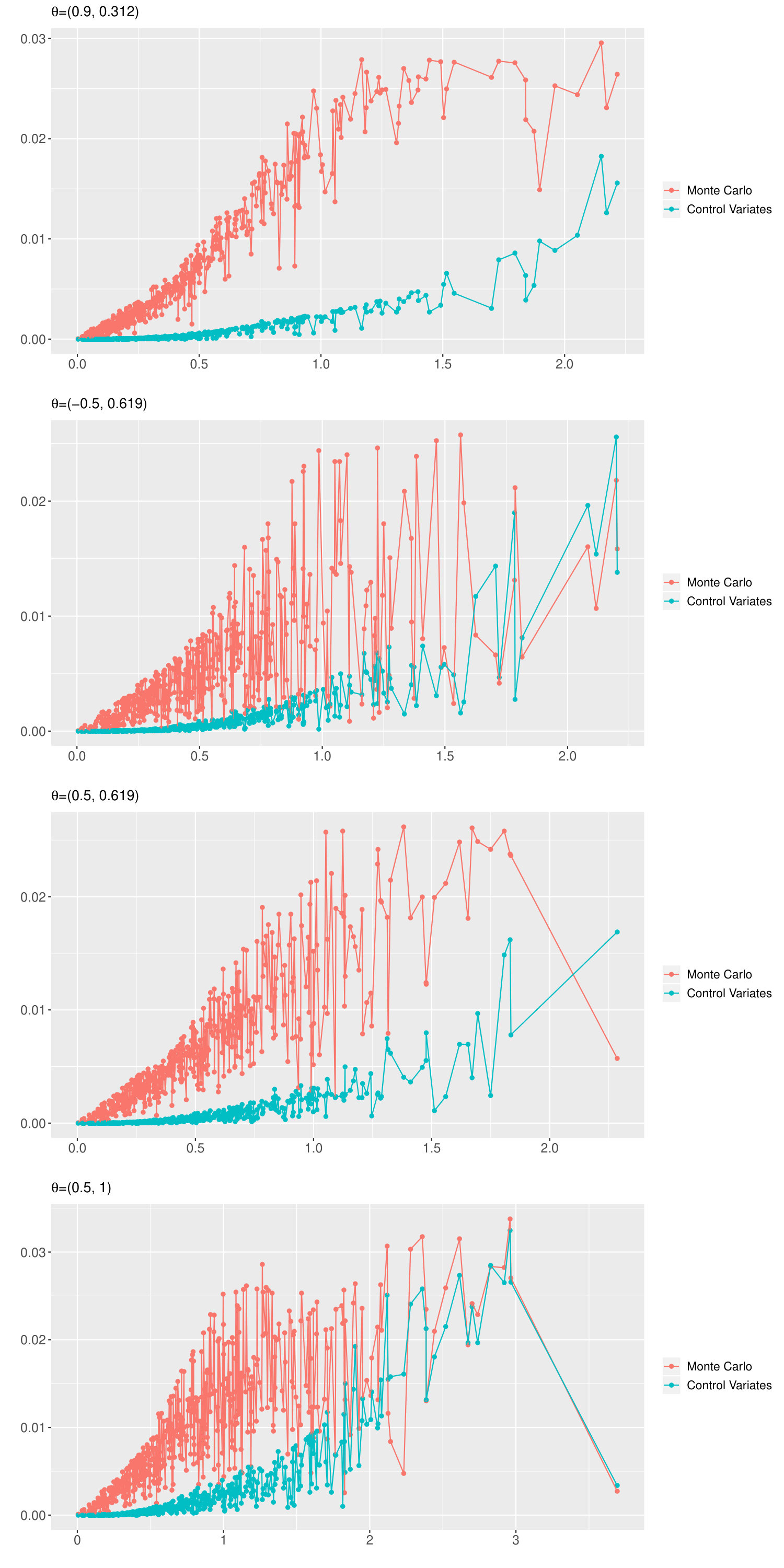 Figure 1
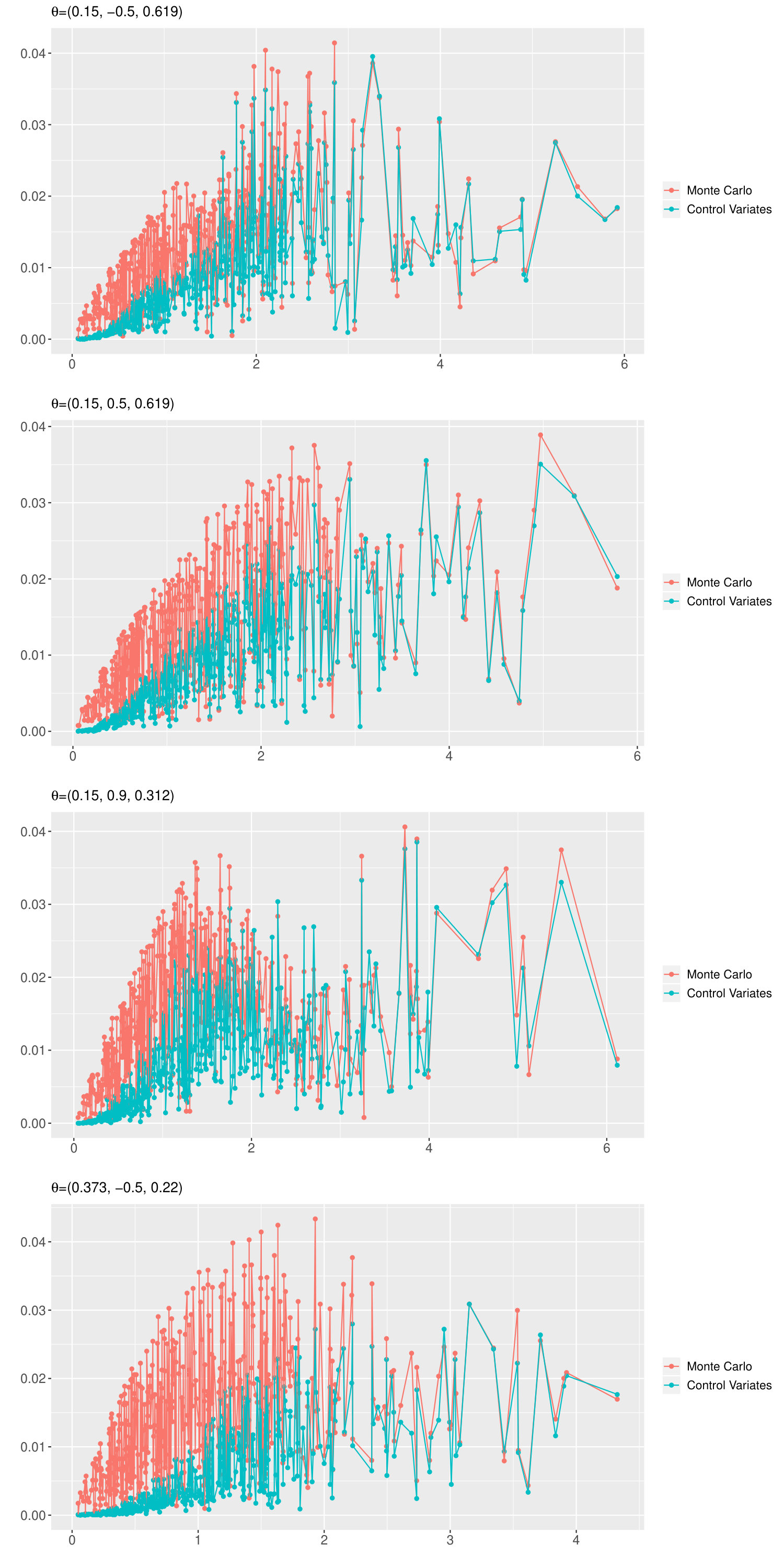 Figure 2
| Bias | Std | RMSE | Bias | Std | RMSE | Bias | Std | RMSE | |
| 0.000 | 0.056 | 0.056 | 0.002 | 0.054 | 0.054 | 0.004 | 0.049 | 0.049 | |
| -0.005 | 0.050 | 0.050 | -0.004 | 0.047 | 0.047 | -0.004 | 0.044 | 0.045 | |
| MLE | -0.015 | 0.040 | 0.043 | -0.015 | 0.040 | 0.043 | -0.016 | 0.040 | 0.043 |
| Bias | Std | RMSE | Bias | Std | RMSE | Bias | Std | RMSE | |
| 0.003 | 0.047 | 0.047 | 0.000 | 0.046 | 0.046 | -0.003 | 0.048 | 0.048 | |
| -0.004 | 0.045 | 0.045 | -0.006 | 0.044 | 0.044 | -0.007 | 0.046 | 0.047 | |
| MLE | -0.016 | 0.040 | 0.043 | -0.017 | 0.039 | 0.043 | -0.017 | 0.039 | 0.043 |
| Bias | Std | RMSE | Bias | Std | RMSE | Bias | Std | RMSE | |
| -0.006 | 0.050 | 0.051 | -0.013 | 0.051 | 0.052 | -0.022 | 0.047 | 0.052 | |
| -0.009 | 0.049 | 0.050 | -0.013 | 0.051 | 0.052 | -0.021 | 0.048 | 0.052 | |
| MLE | -0.019 | 0.039 | 0.043 | -0.021 | 0.037 | 0.043 | -0.027 | 0.034 | 0.043 |
| Bias | Std | RMSE | Bias | Std | RMSE | Bias | Std | RMSE | |
| -0.004 | 0.062 | 0.062 | -0.003 | 0.060 | 0.060 | 0.004 | 0.054 | 0.054 | |
| -0.005 | 0.051 | 0.051 | -0.003 | 0.049 | 0.049 | 0.001 | 0.048 | 0.047 | |
| QMLE | -0.012 | 0.043 | 0.045 | -0.013 | 0.043 | 0.045 | -0.013 | 0.043 | 0.045 |
| 0.008 | 0.049 | 0.050 | 0.012 | 0.051 | 0.053 | 0.012 | 0.049 | 0.051 | |
| 0.005 | 0.047 | 0.047 | 0.009 | 0.046 | 0.047 | 0.010 | 0.046 | 0.047 | |
| QMLE | -0.014 | 0.042 | 0.044 | -0.014 | 0.042 | 0.044 | -0.015 | 0.042 | 0.044 |
| 0.009 | 0.045 | 0.046 | -0.004 | 0.042 | 0.042 | -0.022 | 0.037 | 0.043 | |
| 0.006 | 0.044 | 0.044 | -0.004 | 0.040 | 0.040 | -0.023 | 0.035 | 0.042 | |
| QMLE | -0.016 | 0.041 | 0.044 | -0.019 | 0.039 | 0.044 | -0.025 | 0.035 | 0.043 |
| Bias | Std | RMSE | Bias | Std | RMSE | Bias | Std | RMSE | |
| -0.002 | 0.063 | 0.063 | 0.005 | 0.059 | 0.060 | 0.008 | 0.053 | 0.054 | |
| -0.002 | 0.052 | 0.052 | -0.001 | 0.050 | 0.050 | 0.000 | 0.048 | 0.048 | |
| QMLE | -0.012 | 0.039 | 0.041 | -0.012 | 0.039 | 0.041 | -0.013 | 0.039 | 0.041 |
| 0.008 | 0.049 | 0.050 | 0.004 | 0.050 | 0.050 | 0.008 | 0.050 | 0.050 | |
| 0.001 | 0.047 | 0.047 | 0.002 | 0.047 | 0.047 | 0.001 | 0.047 | 0.047 | |
| QMLE | -0.013 | 0.039 | 0.041 | -0.014 | 0.039 | 0.041 | -0.014 | 0.039 | 0.041 |
| 0.002 | 0.049 | 0.049 | -0.009 | 0.043 | 0.044 | -0.029 | 0.038 | 0.048 | |
| -0.004 | 0.046 | 0.046 | -0.014 | 0.043 | 0.045 | -0.031 | 0.038 | 0.049 | |
| QMLE | -0.016 | 0.038 | 0.041 | -0.018 | 0.037 | 0.041 | -0.024 | 0.033 | 0.041 |
| TRUE | -0.613 | -0.500 | 1.236 | -0.613 | 0.500 | 1.236 | -0.613 | 0.900 | 0.622 |
|---|---|---|---|---|---|---|---|---|---|
| Bias() | -0.015 | 0.025 | 0.002 | -0.012 | 0.014 | -0.032 | -0.016 | -0.010 | 0.002 |
| RMSE() | 0.096 | 0.101 | 0.119 | 0.148 | 0.107 | 0.120 | 0.298 | 0.054 | 0.128 |
| Bias() | 0.023 | 0.031 | -0.007 | 0.006 | 0.002 | -0.018 | 0.061 | -0.007 | -0.036 |
| RMSE() | 0.102 | 0.129 | 0.122 | 0.138 | 0.098 | 0.098 | 0.285 | 0.049 | 0.132 |
| TRUE | 0.150 | -0.500 | 0.619 | 0.150 | 0.500 | 0.619 | 0.150 | 0.900 | 0.312 |
| Bias() | -0.004 | 0.024 | -0.016 | -0.006 | 0.005 | -0.023 | -0.016 | -0.033 | 0.028 |
| RMSE() | 0.057 | 0.144 | 0.088 | 0.074 | 0.141 | 0.081 | 0.147 | 0.084 | 0.095 |
| Bias() | 0.003 | -0.011 | -0.017 | 0.001 | 0.023 | -0.019 | 0.003 | -0.009 | -0.012 |
| RMSE() | 0.055 | 0.124 | 0.085 | 0.071 | 0.102 | 0.069 | 0.145 | 0.062 | 0.087 |
| TRUE | 0.373 | -0.500 | 0.220 | 0.373 | 0.500 | 0.220 | 0.373 | 0.900 | 0.111 |
| Bias() | -0.011 | 0.032 | -0.045 | -0.015 | -0.322 | -0.036 | -0.019 | -0.517 | 0.044 |
| RMSE() | 0.043 | 0.408 | 0.098 | 0.047 | 0.657 | 0.102 | 0.066 | 0.801 | 0.099 |
| Bias() | -0.002 | 0.056 | -0.044 | -0.003 | -0.120 | -0.038 | -0.004 | -0.310 | 0.031 |
| RMSE() | 0.042 | 0.482 | 0.112 | 0.045 | 0.504 | 0.108 | 0.062 | 0.555 | 0.090 |
Peer Reviews
No public reviews on file for this paper yet. If you reviewed it on a platform where reviews are public (OpenReview, ICLR, NeurIPS, ICML), you can paste yours below so the community can read it here.
Videos
No videos yet. Explain this paper in a talk, walkthrough, or lecture? Add one.
Indirect Inference for Time Series Using the Empirical Characteristic Function and Control Variates
Richard A. Davis Department of Statistics, Columbia University, 1255 Amsterdam Avenue, New York, NY 10027, USA, email: [email protected]
Thiago do Rêgo Sousa Center for Mathematical Sciences, Technical University of Munich, 85748 Garching, Boltzmannstr. 3, Germany, email: [email protected], [email protected]
Claudia Klüppelberg22footnotemark: 2
Abstract
We estimate the parameter of a stationary time series process by minimizing the integrated weighted mean squared error between the empirical and simulated characteristic function, when the true characteristic functions cannot be explicitly computed. Motivated by Indirect Inference, we use a Monte Carlo approximation of the characteristic function based on iid simulated blocks. As a classical variance reduction technique, we propose the use of control variates for reducing the variance of this Monte Carlo approximation. These two approximations yield two new estimators that are applicable to a large class of time series processes. We show consistency and asymptotic normality of the parameter estimators under strong mixing, moment conditions, and smoothness of the simulated blocks with respect to its parameter. In a simulation study we show the good performance of these new simulation based estimators, and the superiority of the control variates based estimator for Poisson driven time series of counts.
AMS 2010 Subject Classifications: 62F12, 62G20, 62M10, 65C05, 91G70 ,
Keywords: Asymptotic normality, Characteristic function, Control variates, Indirect Inference estimation, Time series of counts, SLLN, Variance reduction
1 Introduction
Let be a stationary time series, whose distribution depends on for some . Denote by the true parameter, which we want to estimate from observations of the time series. Maximum likelihood estimation (MLE) has been extensively used for parameter estimation, since under weak regularity conditions it is known to be asymptotically efficient. For many models, however, MLE is not always feasible to carry out, due to a likelihood that may be intractable to compute, or maximization of the likelihood is difficult, or because the likelihood function is unbounded on . To overcome such problems, alternative methods have been developed, for instance, the generalized method of moments (GMM) in Hansen (1982), the quasi-maximum likelihood estimation (QMLE) in White (1982), and composite likelihood methods in Lindsay (1988).
In a similar vein, Feuerverger (1990) proposed an estimator based on matching the empirical characteristic function (chf) computed from blocks of the observed time series and the true chf. More specifically, given a fixed , the observed blocks of are
[TABLE]
where . In that paper, a finite set of points in needs to be chosen as arguments for which the true and the empirical chf are compared. However, the practical choice of this set depends on the problem at hand and the asymptotic results derived in Feuerverger (1990) do not offer practical guidance for choosing these points. To overcome this limitation Yu (1998) and Knight and Yu (2002) considered a integrated weighted squared distance between the empirical and the true chfs.
This method has been used in a variety of applications; an interesting review paper, Yu (2004) contains a wealth of examples and references. More recent publications, where the method has been successfully applied to discrete-time models include Knight, Satchell, and Yu (2002), Meintanis and Taufer (2012), Kotchoni (2012), Milovanovic, Popovic, and Stojanovic (2014), Francq and Meintanis (2016), and Ndongo et al. (2016). The method also applies to continuous-time processes after discretization and has been used prominently for Lévy-driven models. The book Belomestny et al. (2015) provides additional insight and references in this field.
The principal goal of this paper is to extend the ideas of these papers to a more general setting. For example, we do not assume the idealized situation for which the chf has an explicit expression as a function of . We propose two new estimators of , which are based on replacing the true chf with estimates that are constructed from a functional approximation of the chf constructed from simulated sample paths of .
While much attention has been given to the choice of the integrated distance used when computing such estimators, which under some regularity conditions can achieve the Cramér-Rao efficiency bound (see eq. (2.3) of Knight and Yu (2002) and Proposition 4.2 of Carrasco et al. (2007)), the focus of our paper is on the practical and theoretical aspects that emerge when it is required to approximate the theoretical chf for parameter estimation. For more details on the search for efficient estimators we refer to Carrasco et al. (2007); Carrasco and Florens (2014); Carrasco and Kotchoni (2017).
Our first estimator is computed from a simple Monte Carlo approximation to replace the true, but unknown chf. This is similar to the simulated method of moments of McFadden (1989) and of the indirect inference method (Smith (1993) and Gourieroux et al. (1993)). In particular, indirect inference has been successfully applied in a variety of situations: parameter estimation of continuous time models with stochastic volatility (Bianchi and Cleur (1996), Jiang (1998), Raknerud and Skare (2012), Laurini and Hotta (2013) and Wahlberg, Welsh, and Ljung (2015)), robust estimation (de Luna and Genton (2001) and Fasen-Hartmann and Kimmig (2020)), and finite sample bias reduction (Gourieroux, Renault, and Touzi (2000, 2010) and Do Rêgo Sousa, Haug, and Klüppelberg (2019)).
More precisely, for many different , we simulate an iid sample of blocks denoted by
[TABLE]
for , and define a simulation based parameter estimator, which minimizes the integrated weighted mean squared error, which is the integrated distance we use, between the empirical chf computed from the blocks (1.2) of the observed time series and its simulated version computed from a large number of simulated paths of the time series.
This is in contrast to the simulation based estimator defined in Section 5.2 of Carrasco et al. (2007), which is computed from one long time series path instead of the iid sample of blocks in (1.2) (a similar method has been applied by Forneron (2018) to estimate the structural parameters and the distribution of shocks in dynamic models). Since we compute the Monte Carlo approximation of the chf from independent blocks, it should have smaller variance than the corresponding one for dependent blocks. Our method gives a chf approximation which yields strongly consistent and asymptotically normal parameter estimators. We also report their small sample properties for different models.
Furthermore, as the Monte Carlo approximation of the chf is computed from iid blocks of a time series, control variates techniques (see Glynn and Szechtman (2002) and Robert and Casella (2004)) provide an even more accurate approximation for the chf. Control variates techniques are classical variance reduction methods in simulation. The idea is to use a set of control variates, which are correlated with the chf. The method then approximates the joint covariance matrix of the control variates and the chf, and uses it to construct a new Monte Carlo approximation of the chf. We choose the first two terms in the Taylor expansion of the complex exponential , and for as control variates, where denotes the usual Euclidean inner product in . This requires knowing the mean and covariance matrix of for .
In assessing the performance of both the Monte Carlo approximation and the control variates approximation of the chf, two trends emerge. First, both the Monte Carlo and the control variates approximations work better for small values of the argument. Second, the control variates approximation performs much better than the Monte Carlo approximation, in particular, for small values of the argument. As a consequence, we propose a control variates based parameter estimator whose integrated mean squared error distinguishes between small and large values of the argument.
Under regularity conditions we prove strong consistency of the proposed parameter estimators and asymptotic normality of the simulation based parameter estimator. We find that the simulation based parameter estimator is asymptotically normal with asymptotic covariance matrix equal to the one of the oracle estimator as derived in Knight and Yu (2002). From this we conclude that there cannot be any improvement in the limit law for the asymptotic normality of the control variates based estimator. However, we prove that it is computed from a better approximation of the chf. Thus, the control variates estimator improves the finite sample performance compared to the simulation based parameter estimator.
It is assumed throughout that is a stationary time series. This ensures that the blocks of random variables in (1.1) are stationary, from which we obtain convergence of the empirical chf to the joint chf. Now in some restricted cases, our method can be adapted to special types of nonstationarity. For example, if is nonstationary, but the differenced process is stationary, then our methodology can be applied directly to . Similarly, if , where is stationary and is a mean function that can be estimated consistently say by , then the methodology can be applied to . We do not pursue this line of investigation here.
The finite sample performance of the estimators are investigated for two important models. We begin with a stationary Gaussian ARFIMA model, whose chf is explicitly known so that we can use the oracle estimator and compare its performance with the simulated based estimator. Their performance is comparable and also very close to the MLE, so in this model there is no need to use control variates. The second example is a nonlinear model for time series of counts, which has been proposed originally in Zeger (1988) and applied, for instance, for modeling disease counts (see also Campbell (1994), Chan and Ledolter (1995) and Davis, Dunsmuir, and Wang (1999)).
In the second example, the oracle estimator does not apply, since the chf of a Poisson-AR process cannot be computed in closed form. For this model and different parameter sets, both the simulation based and the control variates based estimators perform satisfactorily, and the control variates based estimator improves the performance of the simulation based estimator considerably. When compared with the composite pairwise likelihood estimator in Davis and Yau (2011), the control variates based estimator has comparable or even smaller bias.
Our paper is organized as follows. In Section 2 we present the oracle estimator, and the estimators computed from a Monte Carlo approximation and from a control variates approximation of the chf in detail. Here we also motivate the choice of the control variates used. The asymptotic properties of the two new estimators are established in Section 3. As all estimators are computed from true or approximated chf’s we assess their performance in Section 4, first for a Gaussian AR(1) process and then for the Poisson-AR process. Practical aspects of calculating the weighted least squares function are discussed in Section 5, as well as the estimation results for finite samples. In Section 5.1 we compare the oracle estimator, the simulation based parameter estimator and the MLE for a Gaussian ARFIMA model, whereas in Section 5.2 we compare the simulation based parameter estimator and the control variates based estimator for the Poisson-AR process. The proofs of the main results in Section 3, of Lemma 1 of Section 5, and the Tables discussed in Sections 5.1 and 5.2 are provided in the Appendix.
2 Parameter estimation based on the empirical characteristic function
Throughout we use the following notation. For we use the -norm: , where is the complex conjugate of . For and we denote by the -norm, but recall that in all norms are equivalent. For the symbols and denote its real and imaginary part. For a function its Jacobi matrix is given by and .
2.1 The oracle estimator
Let be a stationary time series process, whose distribution depends on for some . Denote by the true parameter, which we want to estimate, and suppose that we observe . Given a fixed , define for the -dimensional blocks
[TABLE]
where . For the observed blocks correspond to , which can be used to calculate the empirical characteristic function (chf), defined as
[TABLE]
Under mild conditions such as ergodicity, converges a.s. pointwise to the true chf for all . We assume that is chosen in such a way that uniquely identifies the parameter of interest . The idea of estimating from a single time series observation by matching the empirical chf of blocks of the observed time series and the true one has been proposed in Yu (1998) and Knight and Yu (2002), and we use the one in Knight and Yu (2002), where the oracle estimator of is defined as
[TABLE]
where
[TABLE]
with suitable weight function such that the integral is well-defined, and chf
[TABLE]
In an ideal situation, has an explicit expression, which is known for all .
2.2 Estimator based on a Monte Carlo approximation of
Unfortunately, a closed form expression of the chf is for many time series processes not available. However, it can be approximated by a Monte Carlo simulation, and an idea borrowed from the simulated method of moments (McFadden (1989), see also Smith (1993) and Gourieroux, Monfort, and Renault (1993) for a similar idea in the context of indirect inference) is to replace by its functional approximation constructed from simulated sample paths of . For many different , we simulate, independent of the observed time series, an iid sample of the blocks in (2.1) denoted by
[TABLE]
for , and define the Monte Carlo approximation of based on these simulations as
[TABLE]
If we replace in (2.4) by , we obtain the simulation based parameter estimator
[TABLE]
where
[TABLE]
with suitable weight function such that the integral is well-defined.
Remark 2.1**.**
An alternative approximation to (2.7) of the chf is based on generating one long time series path and use the empirical chf of the consecutive blocks of -dimensional random variables constructed as in (2.1) (see Carrasco et al. (2007)). While being unbiased, the approximation will generally have larger variance than the approximation (2.7). Nevertheless, when it is expensive to generate realizations even of dimension , for instance, when a long burn-in time is required to achieve stationarity, it may be computationally more efficient to generate one long time series. While we do not pursue this approach here, the technical aspects of working with one long time series are not much different than the estimate based on independent replicates as in (2.7), but might require a much larger sample size than desired to control the variance of the estimate. This is especially true for long-memory time series.
Since is based on iid time series blocks, we can reduce its variance further using control variates to produce an even more accurate approximation for the chf. This will result in an improved version of .
2.3 Estimator based on a control variates approximation of
The estimator in (2.8) requires only that the stationary time series process can be simulated, and is therefore easily applicable to a large class of models. When computing of (2.9), it is very important that the error
[TABLE]
in approximating the true chf is small, since it propagates to . In order to reduce the variance of the empirical chf , we use the method of control variates, an often used variance reduction technique in the context of Monte Carlo integration (Glynn and Szechtman (2002), Oates, Girolami, and Chopin (2017), Portier and Segers (2019)).
We construct a control variates approximation of from the iid sample , , as in (2.6). We also require explicit expressions for the moments for and .
Recall that for all , so that both random variables have the same moments. As in Portier and Segers (2019), we denote by the distribution of the block and by its empirical version. For example, if for , we want to provide a good approximation for for . To apply the control variates technique, we need control functions, which are correlated with and whose expectations are known. In the time series context, it is often that we know the first and second order structure of the process in closed form. Even for complicated models, e.g., models defined in terms of stochastic integrals (see e.g. Brockwell (2001); Klüppelberg et al. (2004); Brockwell et al. (2006); Stelzer (2010)) these expressions are available. The first and second order of appear in the Taylor series of and therefore they are natural choices of control functions. We also remark that if the time series process also allows for the computation of additional moments expressions in closed form, which are correlated with , then we encourage using them as control functions while approximating the chf. We describe now the construction of the control variates approximation in detail.
We use the first two terms in the Taylor series of the complex function , which suggests the vector of control functions , where for ,
[TABLE]
so that , the zero vector in . The Monte Carlo approximation of based on the iid sample , , is then
[TABLE]
Since , the Monte Carlo approximation is unbiased and has variance
[TABLE]
Then for every vector , we have that is also an unbiased estimator of . Since , , is an independent sample, and, if we differentiate the map with respect to and set it equal to zero, we obtain (cf. Approach 1 in Glynn and Szechtman (2002)) the theoretical optimum
[TABLE]
provided the inverse exists. In this case, the estimator
[TABLE]
has minimal asymptotic variance. In order to investigate the existence of the above inverse note that for each fixed and , the determinant of is
[TABLE]
Since by the Cauchy-Schwarz inequality,
[TABLE]
it follows (see e.g. Klenke (2013), Theorem 5.8) that
[TABLE]
for some with . As the scalar product is random, universal coefficients to satisfy the right-hand side of (2.15) exist only in degenerate cases, which we do not consider.
Since is unknown, it needs to be estimated (e.g. by one of the methods in Glynn and Szechtman (2002), and we use the one described in eqs. (6) and (7) in Portier and Segers (2019)):
[TABLE]
For the iid sample , as in (2.6) we obtain the control variates approximation of given by
[TABLE]
where
[TABLE]
Recall from (2.11) that , so we could simply replace in (2.9) by as given in (2.17). However, as we shall see in Section 4, the control variates approximation provides superior approximations of only for values of , for which is small. Thus, we replace in (2.9) by a combination of and . More precisely, we propose the following control variates based estimator:
[TABLE]
where for appropriate ,
[TABLE]
, with suitable weight function such that the integral is well-defined.
It is worth mentioning that, for a fixed weight function , the weight function can always be computed since depends only on the time series data. The downside of using the control variates based estimator (2.19) is that one needs to resort to numerical integration. However, the procedure is feasible for moderate dimension . As illustrated in the Poisson-AR example of Section 4.2, the control variates based estimator has improved the performance over the simulation based estimator (2.8) considerably.
Note that where with
[TABLE]
and . The choice of the indicator function is justified by the fact that, when estimating the parameter , we focus on approximations of for close to .
3 Asymptotic behavior of the parameter estimators
Before performing the parameter estimation we need to make sure that the parameters are identifiable from the model.
In the following we assume that the model parameters are identifiable from the chf. In our examples, the dimension must be at least 2. For a specific choice of , the minimum in (2.19) may not be unique giving an identifiability problem of the estimated model. This may be remedied by increasing the dimension .
In the sequel, we will make various assumptions on different aspects of the underlying process, smoothness of the model, moments of the process, and properties of the weight function. We group these assumptions into the following categories.
Assumptions A** (Parameter space and time series process).**
**
* is a compact subset of and , the interior of .* 2.
* is a stationary and ergodic sequence.* 3.
* is -mixing with rate function satisfying for some .*
Assumptions B** (Continuity and differentiability in ).**
**
For each , the map is continuous on . 2.
For each , the map is twice continuously differentiable in an open neighborhood around .
Assumptions C** (Moments).**
**
, where with being such that holds. 2.
* for some where with being such that holds.* 3.
. 4.
For each , . 5.
* and for some .*
Assumptions D** (Weight function).**
**
. 2.
. 3.
* for some .* 4.
.
Assumption B is indeed satisfied by many linear and non-linear time series processes, in particular, when they have a representation or
for iid noise variables , and is a measurable function. Prominent examples are the MA and AR representations of a causal or invertible ARMA model (see e.g. eqs. (3.1.15) and (3.1.18) in Brockwell and Davis (2013)) or the ARCH representation of a GARCH model (see e.g. Francq and Zakoïan (2011), Theorem 2.8). In this case, assumptions and will hold whenever the map is continuously differentiable for . For example, if is Lipschitz-continuous for , then the continuity assumption holds.
The key asymptotic properties, consistency and asymptotic normality of our estimates are stated in the following theorems. The proofs of these results are presented in the Appendix.
We formulate first the strong consistency results of the parameters.
Theorem 3.1** (Consistency of ).**
Assume that , , , and hold. Let as . Then as
Theorem 3.2** (Consistency of ).**
Assume that the conditions of Theorem 3.1 hold, and additionally , , and . Let as . Then as
The asymptotic normality of the simulation based parameter estimator reads as follows.
Theorem 3.3** (Asymptotic normality of ).**
Assume that Assumptions A and B, and the moment conditions , , and hold. Furthermore, assume that the weight function satisfies , and . Set and as and define
[TABLE]
and
[TABLE]
If is a non-singular matrix, then
[TABLE]
where
[TABLE]
Theorem 3.3 shows that is asymptotically normal and achieves the same asymptotic efficiency as the oracle estimator from (2.3) (see Theorem 2.1 in Knight and Yu (2002)). Therefore, there cannot be any improvement in the limit law for the asymptotic normality of . However, as we show in Section 4, is based on a better approximation of the chf than that used for . Thus, the control variates estimator improves the finite sample performance compared to the simulation based estimator .
Remark 3.4**.**
As pointed out in (Knight and Yu, 2002, Remark 2.3), the asymptotic variance of in (3.3) can be approximated by replacing by in (3.2) and (3.4) and by replacing the infinite sum in (3.4) by an approximating sum with a kernel and a convenient bandwidth using the methods suggested in Andrews (1991) and Newey and West (1994).
4 Assessing the quality of the estimated chf
In this section we compare the performance of both the Monte Carlo approximation and the control variates approximation of the chf as defined in (2.7) and (2.17), respectively. We start with the following comparison of the two chf approximations.
Remark 4.1**.**
[Comparison of and ] Assume that holds, and let and be as defined in (2.14) and (2.17), respectively. We use that as with limit given in (2.13). This follows from the representation of as
[TABLE]
and the almost sure convergence of both terms. The quantities needed to compute the estimator in (2.16) are, for each :
[TABLE]
Hence, strong consistency of follows from the SLLN. This together with implies by Theorem 1 in Glynn and Szechtman (2002) that, as ,
[TABLE]
[TABLE]
with
[TABLE]
[TABLE]
with as defined in (2.12). Therefore, provides an approximation of the integral in (2.4) with smaller variance than . As a consequence, this favors the control variates estimator over the simulation based estimator for large sample sizes .
For all forthcoming examples we choose and . We begin with a stationary Gaussian AR(1) process, where we know the chf explicitly, and then proceed to the Poisson-AR process, where we approximate the true unknown chf by a precise simulated version.
4.1 The Gaussian AR(1) process
We start with a stationary Gaussian AR(1) process to show how the method of control variates improves the Monte Carlo approximation of its chf. Let be the AR(1) process
[TABLE]
with parameter space being a compact subset of . Then the true chf of is given by for where the covariance matrix is explicitly known and identifies the parameter uniquely; see e.g. Brockwell and Davis (2013), Example 3.1.2. For a fixed and many we compute the absolute errors
[TABLE]
where is the Monte Carlo approximation of the chf of and its control variates approximation. To understand how well we can approximate , we plot in Figure 1, and against for different parameters . These quantities are computed from an iid sample as in (2.6). To simulate iid observations from the model (4.3), we use the fact that the one-dimensional stationary distribution is , and then use the recursion in (4.3) to simulate and . We chose randomly generated values of from the -dimensional Laplace distribution with chf given in (5.2).
It is clear from Figure 1 that both the Monte Carlo and the control variates approximations work better when is small, and also that the control variates approximations are best for small values of . The superiority of the control variates approximation for all and all parameter settings is clearly visible, and already expected from Remark 4.1.
4.2 The Poisson-AR model
We consider a nonlinear time series process for time series of counts, which has been proposed originally in Zeger (1988). A prototypical Poisson-AR(1) model suggested in Davis and Rodriguez-Yam (2005) assumes that the observations are independent and Poisson-distributed with means where the process is a latent stationary Gaussian AR(1) process, given by the equations
[TABLE]
with parameter space being a compact subset of . The parameter is uniquely identifiable from the second order structure, which has been computed in Section 2.1 of Davis, Dunsmuir, and Wang (2000).
For this model, the true chf of cannot be computed in closed form. To mimic the assessment of the errors in eq. (4.4), we simulate iid observations from by first simulating a Gaussian AR(1) process (as described in Section 4.1) and then simulating independent Poisson random variables with means , and , respectively. From this we compute the empirical characteristic function and take it as in the absolute error terms (4.4).
We compare the performance of both the Monte Carlo approximation and the control variates approximation of the chf. Figure 2 presents the results. The plots in Figure 2 are also in favor of the control variates approximation, when compared to the Monte Carlo approximation.
5 Practical aspects and simulation results
Our objective is to obtain a simple expression of the integrated mean squared error in (2.9), which is needed to compute the estimator in (2.8). For a weight function in (2.9), we write
[TABLE]
for its Fourier transform. Our preference is on weight functions such that (5.1) is known explicitly.
Example 5.1**.**
[Weight functions and their characteristic functions]
(i) Laplace: is a multivariate Laplace density with chf
[TABLE]
(ii) Cauchy: is a multivariate Cauchy density with chf
[TABLE]
(iii) Gaussian: is a standard multivariate Gaussian density with chf
[TABLE]
Lemma 5.2**.**
Let be as in (2.9) and a weight function with Fourier transform . Then
[TABLE]
Formula (5.4) is very useful, since it avoids the computation of a -dimensional integral. Additionally, since the first double sum on the right-hand side of (5.4) does not depend on the argument , for the optimization it can be ignored.
Remark 5.3**.**
When evaluating the integrated weighted mean squared errors (2.9), (2.20), or (5.4) in practice, they need to be deterministic functions of . This is enforced by taking a fixed seed for every , when simulating for different values of .
In the following two examples we study the finite sample behavior of the estimators and . We begin with a stationary Gaussian ARFIMA model, whose chf is explicitly known so that we can use the oracle estimator from Section 2.1. Afterwards we come back to the Poisson-AR process. We choose , since the 3-dimensional chf contains sufficient information to identify the parameter of interest. We also choose .
5.1 The ARFIMA model
Let be the stationary Gaussian ARFIMA model
[TABLE]
where is the backshift operator, with parameter space being a compact subset of . Then the true chf of is given by for where the covariance matrix is explicitly known and identifies the parameter uniquely; see e.g. Pipiras and Taqqu (2017), Corollary 2.4.4.
For the long-memory case, for each value of we compare the new estimators with the MLE method as implemented in the R package arfima. Thus, for many , we generate iid Gaussian random vectors with mean zero and covariance and use them to construct the simulation based estimator .
Since the chf is known in closed form, we are able to compute the oracle estimator from (2.4). In order to compute the integral appearing in (2.4) in closed form, we choose the weight function .
Then the integral in (2.4), which needs to be minimized with respect to the parameter , can be evaluated similarly as in (5.4), giving for the chf being known, that can be written as
[TABLE]
We compare in Table 1.1 the performance of the simulation based estimator , the oracle estimator in (2.3) based on the minimization of (5.1), and the MLE. We fixed for all simulated sample paths used in the simulation study. For both and , we also estimate but report only the performance for the estimator of which is the key parameter of interest in long-range dependence models. We notice that is comparable to the oracle estimator, so in this model there is no need to use control variates. When comparing both simulation based estimators, the RMSEs are almost the same for all . The MLE has a smaller RMSE, but both and have a smaller bias than the MLE. In the simulations, the density plots for the estimates of with look reasonably normal. On the other hand, the estimates when is closer to are rather skewed, which is expected due to the constraint . In this case a larger sample is needed in order to obtain more normal looking densities.
Remark 5.4**.**
We also investigate the feasibility of our new estimation procedures for misspecified models. We take a Gaussian ARFIMA as the true model, but for the data we modify the distribution of its innovations. Specifically, we consider the two cases of ARFIMA models driven by noise with a Laplace distribution and with a Student- distribution with 6 degrees of freedom. The estimation results under the two misspecification scenarios are shown in Tables 1.2 and 1.3 of the Appendix. The quasi-oracle estimator is based on the Gaussian chf, and the quasi-MLE (QMLE) is found by maximizing the Gaussian likelihood, even though the data are in fact nonGaussian. For both noise distributions, we see very little difference in the performance of the three estimators (QMLE compared with MLE) from the Gaussian ARFIMA scenario in Table 1.1. In particular, our estimator continues to have small bias and RMSE that is comparable to the oracle estimator and only slightly larger than that of the QMLE. Of course, it is known that the QMLE estimators behave asymptotically the same as the MLE when the data is Gaussian.
5.2 The Poisson-AR process
The Poisson-AR model has been defined in Section 4.2. We conduct a simulation experiment in the same setting as in Table 5 in Davis and Rodriguez-Yam (2005) and Table 3 in Davis and Yau (2011). The results are shown in Table 1.4 of the Appendix for and nine different parameter settings, where we also classify the models by the corresponding index of dispersion of the random variable , which assumes values in as shown in Davis and Rodriguez-Yam (2005).
We compare both the simulation based estimator and control variates based estimator . We fix , and the -dimensional Laplace density as in (5.2) for . To simulate iid observations of we proceed as explained in Section 4.2. The simulation based estimator in (2.8) is computed via (5.4). Unfortunately, such a formula cannot be obtained for the control variates based estimator , since the introduction of the correction in (2.18) introduces additional polynomial terms into in (2.20). Thus, we resort to numerical integration to evaluate .
Our findings are as follows. For , the control variates based estimator for presents smaller bias and RMSE than the simulation based estimator in most cases, in all others it is comparable. The smallest RMSE values are shaded in Table 4. Additionally, a significant improvement in the bias for estimating is noticeable for and . This example shows the advantage of using control variates to improve the estimation of the model parameters. This is not surprising in view of the improved performance of estimating the characteristic function as seen in all three panels of Figure 2.
We compare now the control variates based estimator in Table 2 of the Appendix, with the results for the consecutive pairwise likelihood (CPL) from Table 3 in Davis and Yau (2011), which is referred to as CPL1 in that paper. The bias of is smaller than that of CPL1 for the estimated and for almost all cases, in all others it is comparable. For the bias of and CPL1 are comparable, except that shows poor performance for estimating for the true parameter . This is due to the fact that the simulated sample paths contain a large number of zeros, giving very little information for the parameter estimation. The estimated values for look normal for all parameter choices. The sampling distributions of the other parameter estimates look close to normal, except in the boundary. In particular, the density for the estimates of when or and estimates of when show some asymmetry, deviating from normality. This is not unexpected because they are close to the boundary.
Appendix A Appendix
Here we present the proofs of the main Theorems, as well as tables of results on the simulation study. Then, in Section A.1 we provide the proofs of Theorems 3.1, 3.2, and 3.3. Finally, we present in Section A.2 the tables summarizing the finite sample behavior of the simulation based estimators for ARFIMA models driven by noise from Gaussian, Laplace, and Student- distributions, and the Poisson-AR(1) model discussed in Section 5.
A.1 Proofs of the main results
In the following we define and , but omit the argument for notational simplicity. Throughout the letter stands for any positive constant independent of the respective argument. Its value may change from line to line, but is not of particular interest. For a matrix with only real eigenvalues denotes the smallest eigenvalue.
We often use the uniform SLLN, which guarantees for a continuous stochastic process satisfying that
as for every compact set . More precisely, we use the SLLN on the separable Banach space , the space of continuous functions on the compact set , endowed with the sup norm (see e.g. Theorem 16(a) in Ferguson (1996) or Theorem 9.4 in Parthasarathey (1967)).
Proof of Theorem 3.1: Let
[TABLE]
be the candidate limiting function of . For define the set
[TABLE]
Since for all and , and the random elements are iid, the uniform SLLN holds giving
[TABLE]
In particular, for we also have
[TABLE]
Applying the inequality for gives
[TABLE]
Applying on both sides of (A.4), using (A.2) combined with , and taking the limit for gives
[TABLE]
Now we prove that if and only if . Obviously . If , then the distributions of and are different and thus also their characteristic functions are different. Since characteristic functions are continuous, it follows that they are different at least on an interval with positive Lebesgue measure; hence . Therefore, is uniquely minimized at and this fact together with (A.5) gives strong consistency of .
Proof of Theorem 3.2: We have that , with being the -dimensional empirical covariance matrix of the observed time series as in (2.21). Let be fixed and
[TABLE]
be the candidate limiting function of in (2.20), where is the theoretical -dimensional covariance matrix of the time series process .
Based on the definition of in (2.20), we divide the domain of integration in the integrated mean squared error into and , equivalently into and its complement .
Recall also (2.17) and (2.18). Using for all , together with for gives for the integral on :
[TABLE]
[TABLE]
By and it follows from Theorem 3(a) in Section 1.2.2 of Doukhan (1994) that
[TABLE]
Since , it follows from (A.7) combined with Proposition 5.1.1 in Brockwell and Davis (2013) that , and therefore, the minimum eigenvalue of is positive. Thus, for all ,
[TABLE]
By and the ergodic theorem and, since the eigenvalues of a matrix are continuous functions of its entries (cf. Bernstein (2009), Fact 10.11.2), also . It follows from (A.8) and from the a.s. convergence of the eigenvalues that there exists such that
[TABLE]
Thus, for we obtain
[TABLE]
This together with (A.10) gives the following upper bound for the right-hand side of (A.6):
[TABLE]
The first integral can be estimated as in (A.4) which tends to 0 uniformly for provided that holds. Since , also the second integral in (A.11) tends 0 a.s. as .
We turn to the integrated mean squared error on . Let . The control variates correction used in (2.20) can be regarded as a continuous function whose entries are the arithmetic means defined in (4.1)-(4.2). By and the uniform SLLN, each of these arithmetic means converge a.s. uniformly on as and . Thus, it follows from the continuity of and the continuous mapping theorem that
[TABLE]
For it follows from (A.9) that and thus using the inequality
[TABLE]
valid for with gives
[TABLE]
From (A.8), (A.12), (A.2), and (A.3) with for ) ,and it follows that as . Finally,
by similar arguments as used in (A.10) and (A.11), since for , also applying ,
[TABLE]
and
[TABLE]
Proof of Theorem 3.3: By the definition of in (2.8) and under assumptions and we have
[TABLE]
A Taylor expansion of order 1 of around gives
[TABLE]
where as . Therefore, asymptotic normality of will follow by the delta method, if we prove that as :
converges weakly to a multivariate normal random variable, and 2.
converges in probability to a non-singular matrix.
We start with the first point and compute the partial derivatives of :
[TABLE]
Recall that and denote the empirical characteristic functions of the observed blocks as in (2.2) and of its Monte Carlo approximation as in (2.7), respectively. Define the partial derivatives of the real and imaginary part of :
[TABLE]
and summarize them into
[TABLE]
Then consider
[TABLE]
Abbreviate and . Then it follows from (A.13), (A.15) and (A.16) that
[TABLE]
We analyze the asymptotic behavior of the first term in (A.17) in Lemma A.3. More precisely, we show there that for as in (A.1) converge in distribution to a -dimensional Gaussian vector. Afterwards, Lemmas A.4 and A.5 show that as , componentwise in ,
[TABLE]
and
[TABLE]
where is a zero mean -valued Gaussian field. The formula given in (A.17) tells us that the term will appear in the asymptotic covariance formula of the limiting distribution of the estimator. Therefore it is worth writing it in terms of the chf (2.5).
Remark A.1**.**
For each and , it follows from (A.14) that
[TABLE]
Since both and are bounded by we can use to interchange expectation and differentiation in (A.18). This combined with (A.15) gives
[TABLE]
This remark will be used later in the proof of Theorem 3.3.
We show by a standard Chebyshev argument that the second term in (A.17) converges in probability componentwise to 0 in (A.48). The convergence of the second derivatives will be the topic of Lemma A.6. For the scalar products above we use the following bounds several times below.
Lemma A.2**.**
Let , , and be fixed and assume that holds.Then the following bounds hold true.
- (a)
If for , then there exists a constant such that
[TABLE]
- (b)
If for , then there exists a constant such that
[TABLE]
The same bounds hold uniformly, taking expectations over or over for some compact at both sides of (A.20) and (A.21), provided the corresponding expectations exist.
Proof.
(a) Applying the Cauchy-Schwarz inequality for the inner product, the fact that , bounding the -norm by the -norm, employing the inequality valid for and gives
[TABLE]
Part (b) follows by analogous calculations. ∎
Lemma A.3**.**
Under assumptions , , , and we have on the Borel sets of ,
[TABLE]
where is an -valued Gaussian field.
Proof.
Under assumptions and , it follows from Lemma 4.1(2) in Davis et al. (2018) that convergences in distribution on compact subsets of to a complex-valued Gaussian field , equivalently the vector of real and imaginary part converge to a bivariate Gaussian field . Since the random elements are iid and the partial derivatives exist by , also are iid. Then it follows from the definitions (A.14), (A.15), and Lemma A.2 with in combination with that
[TABLE]
Hence, the uniform SLLN guarantees that
[TABLE]
Slutsky’s theorem gives then convergences in distribution on compact subsets of to as . The result in (A.23) follows from the continuity of the integral by another application of the continuous mapping theorem on . ∎
Lemma A.4**.**
Under assumptions , and we have componentwise in ,
[TABLE]
Proof.
Since and are independent and , we have for all . An application of the Cauchy-Schwartz inequality for integrals gives
[TABLE]
We first obtain a bound for the product between the first component of and the first component of . Define for
[TABLE]
Then,
[TABLE]
Under it follows from Theorem 3(a) in Section 1.2.2 of Doukhan (1994) that for fixed ,
[TABLE]
where and, thus, it follows from the stationarity of combined with (A.28) and the fact that that
[TABLE]
where the bound is independent of . Recall that . Under , it follows from the iid property of
[TABLE]
Using the fact that \Big{|}\frac{1}{n}\sum_{j=1}^{n}U_{j}(t)\Big{|}\leq 2, adding and subtracting with the inequality , and (A.30) gives
[TABLE]
The calculations in (A.29), (A.30), and (A.31) can now be applied to show that for all ,
[TABLE]
and, thus, it follows from (A.26) together with and that
[TABLE]
∎
Lemma A.5**.**
[TABLE]
Proof.
It follows from (A.14), (A.15), , and (A.24)
Now we find an upper bound for the variance of each component of for a fixed . Let be as defined at the left-hand side of (A.27) and notice that the first component of is the distributional limit of . Since is -mixing by , we can apply the CLT in Ibragimov and Linnik (1971) (Theorem 18.5.3 with ) and find that the variance of the first component of is given by
[TABLE]
This combined with Theorem 3(a) in Section 1.2.2 of Doukhan (1994) and the fact that and for all gives by and (A.28)
[TABLE]
A similar calculation shows that the variance of the second component of is also bounded by a finite constant, which does not depend on . Therefore, . This combined with (A.24) and assumption gives
[TABLE]
Since -convergence implies convergence in probability the result follows. ∎
This proves part (1) of the delta method. We now turn to part (2). In order to calculate the second derivatives of , which exist by , we rewrite (A.13) as
[TABLE]
For the second derivatives we calculate for every ,
[TABLE]
where we summarize all quantities used in the following list:
[TABLE]
[TABLE]
Lemma A.6**.**
If the assumptions , , , , hold and satisfying , then for every , as
[TABLE]
Proof.
We first prove that as
[TABLE]
Step 1: Uniform convergence on : It follows from the iid property of the random elements that the sequence
is iid. Lemma A.2 together with gives the uniform bound
[TABLE]
and it follows from the uniform SLLN that for every fixed
[TABLE]
Similarly,
[TABLE]
Because of the ergodic theorem gives
[TABLE]
Therefore, (A.37) combined with (A.38) and the triangle inequality imply
[TABLE]
Step 2: Pointwise convergence of : The triangle inequality implies
[TABLE]
Since and the map is continuous in , (by and ) it follows that the second term on the right-hand side of (A.40) converges a.s. to zero. Additionally, since the uniform convergences on (A.36) and (A.39) imply the uniform convergence of the product on it follows that the first term on the right-hand side of (A.40) also converges a.s. to zero.
Step 3: -convergence: Since we have already shown a.s. convergence, it follows from Theorems 6.25(iii) and 6.19 in Klenke (2013) (with ) that -convergence follows provided that
[TABLE]
for some . Using the fact that and the inequality , , we obtain
[TABLE]
since . Now we use the inequality for , assumption for the uniform bound in Lemma A.2 and the fact that the sequence is iid to continue
[TABLE]
Step 4: Convergence of the random integrals: Define the sequence of functions
[TABLE]
and recall that from the -convergence showed in Step 3, for every we have as . From the definition of the function in the last line of (A.42) it follows that . Additionally, assumption implies that
[TABLE]
Therefore, it follows from Fubini’s Theorem and dominated convergence that
[TABLE]
and therefore the convergence in probability of (A.35) follows from the -convergence in (A.43).
The proofs for the other three remaining integrals on the right-hand side of (A.33) follow along the same lines. The result in (A.34) is then a consequence of the fact that for all , . ∎
Proof of Theorem 3.3: We handle each term in (A.17) separately. As a direct consequence of Theorem 3.1 and Lemmas A.3-A.6,
[TABLE]
where with
[TABLE]
[TABLE]
and being the -valued Gaussian field from Lemma A.3. For arbitrary we have
[TABLE]
Since is -mixing by , we can apply the CLT in Ibragimov and Linnik (1971) (Theorem 18.5.3 with ) and find that
[TABLE]
where
[TABLE]
Substituting (A.46) and (A.47) into (A.45) gives with Fubini’s Theorem
[TABLE]
which combined with Remark A.1 gives (3.4). By the same arguments of interchanging expectation and differentiation from Remark A.1 we obtain
[TABLE]
This together with (A.44) gives
[TABLE]
leading to (3.2).
The second term in (A.17) is, up to a constant,
[TABLE]
It follows from the fact that combined with (A.32) that
[TABLE]
as . Thus (3.3) follows from Chebyshev’s inequality.
A.2 Finite sample behavior of the estimators
A.2.1 ARFIMA models driven by noise from Gaussian, Laplace, and Student- distributions
A.2.2 Poisson-AR model
Data sharing: Data sharing is not applicable to this article as no datasets were analyzed or used in this study.
Acknowledgement
Thiago do Rêgo Sousa gratefully acknowledges support from the National Council for Scientific and Technological Development (CNPq - Brazil) and the TUM Graduate School. He also thanks the Statistics Department at Columbia University for its hospitality during his visit and takes pleasure to thank Viet Son Pham and Thibaut Vatter for helpful discussions. Davis’ research was partially supported by NSF grant DMS 2015379 to Columbia University.
The reference list from the paper itself. Each links out to its DOI / PubMed record.
- 1Andrews (1991) D. W. Andrews. Heteroskedasticity and autocorrelation consistent covariance matrix estimation. Econometrica: Journal of the Econometric Society , pages 817–858, 1991.
- 2Belomestny et al. (2015) D. Belomestny, F. Comte, V. Genon-Catalot, H. Masuda, and M. Reiß. Estimation for Discretely Observed Lévy Processes . Lévy Matters IV (LN in Mathematics, Vol. 2128). Springer, Cham, 2015.
- 3Bernstein (2009) D. S. Bernstein. Matrix Mathematics: Theory, Facts, and Formulas . Princeton University Press, Princeton, 2009.
- 4Bianchi and Cleur (1996) C. Bianchi and E. M. Cleur. Indirect estimation of stochastic differential equation models: some computational experiments. Computational Economics , 9(3):257–274, 1996.
- 5Brockwell et al. (2006) P. Brockwell, E. Chadraa, A. Lindner, et al. Continuous-time garch processes. The Annals of Applied Probability , 16(2):790–826, 2006.
- 6Brockwell (2001) P. J. Brockwell. Lévy-driven carma processes. Annals of the Institute of Statistical Mathematics , 53(1):113–124, 2001.
- 7Brockwell and Davis (2013) P. J. Brockwell and R. A. Davis. Time Series: Theory and Methods . Springer, New York, 2013.
- 8Campbell (1994) M. Campbell. Time series regression for counts: an investigation into the relationship between sudden infant death syndrome and environmental temperature. Journal of the Royal Statistical Society. Series A , pages 191–208, 1994.