An Analysis of Speech Enhancement and Recognition Losses in Limited Resources Multi-talker Single Channel Audio-Visual ASR
Luca Pasa, Giovanni Morrone, Leonardo Badino

TL;DR
This paper investigates how joint training of speech enhancement and recognition models impacts performance in multi-talker audio-visual scenarios, revealing complex interactions and improvements in phone error rates.
Contribution
It introduces and analyzes joint end-to-end models for speech enhancement and recognition in multi-talker settings, highlighting training strategies and their effects.
Findings
Joint optimization reduces Phone Error Rate significantly.
Speech enhancement capability decreases during ASR training.
Models trained jointly outperform baseline models trained separately.
Abstract
In this paper, we analyzed how audio-visual speech enhancement can help to perform the ASR task in a cocktail party scenario. Therefore we considered two simple end-to-end LSTM-based models that perform single-channel audio-visual speech enhancement and phone recognition respectively. Then, we studied how the two models interact, and how to train them jointly affects the final result. We analyzed different training strategies that reveal some interesting and unexpected behaviors. The experiments show that during optimization of the ASR task the speech enhancement capability of the model significantly decreases and vice-versa. Nevertheless the joint optimization of the two tasks shows a remarkable drop of the Phone Error Rate (PER) compared to the audio-visual baseline models trained only to perform phone recognition. We analyzed the behaviors of the proposed models by using two…
Click any figure to enlarge with its caption.
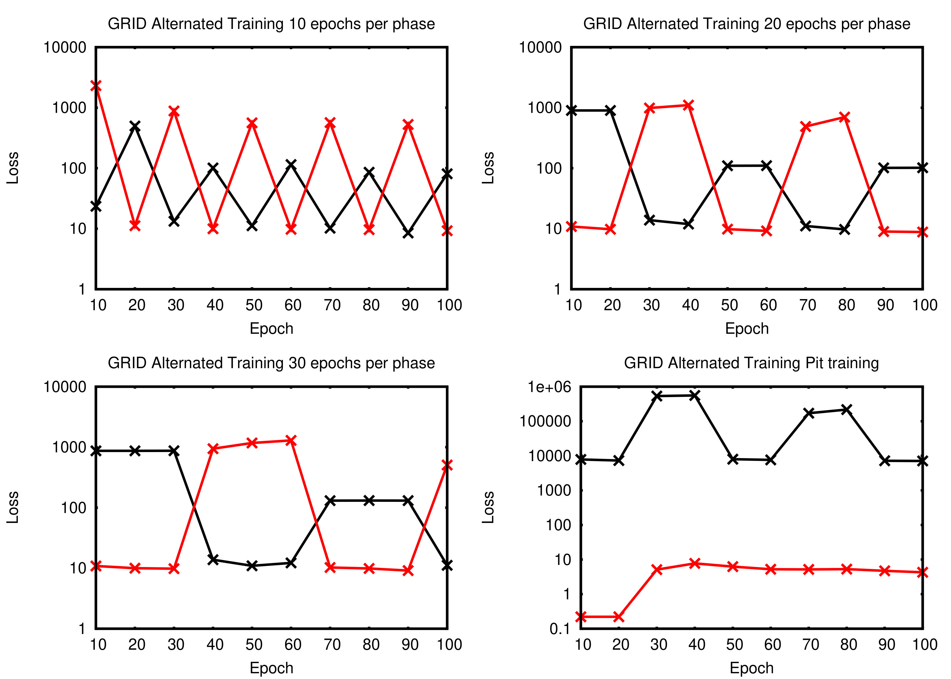 Figure 1
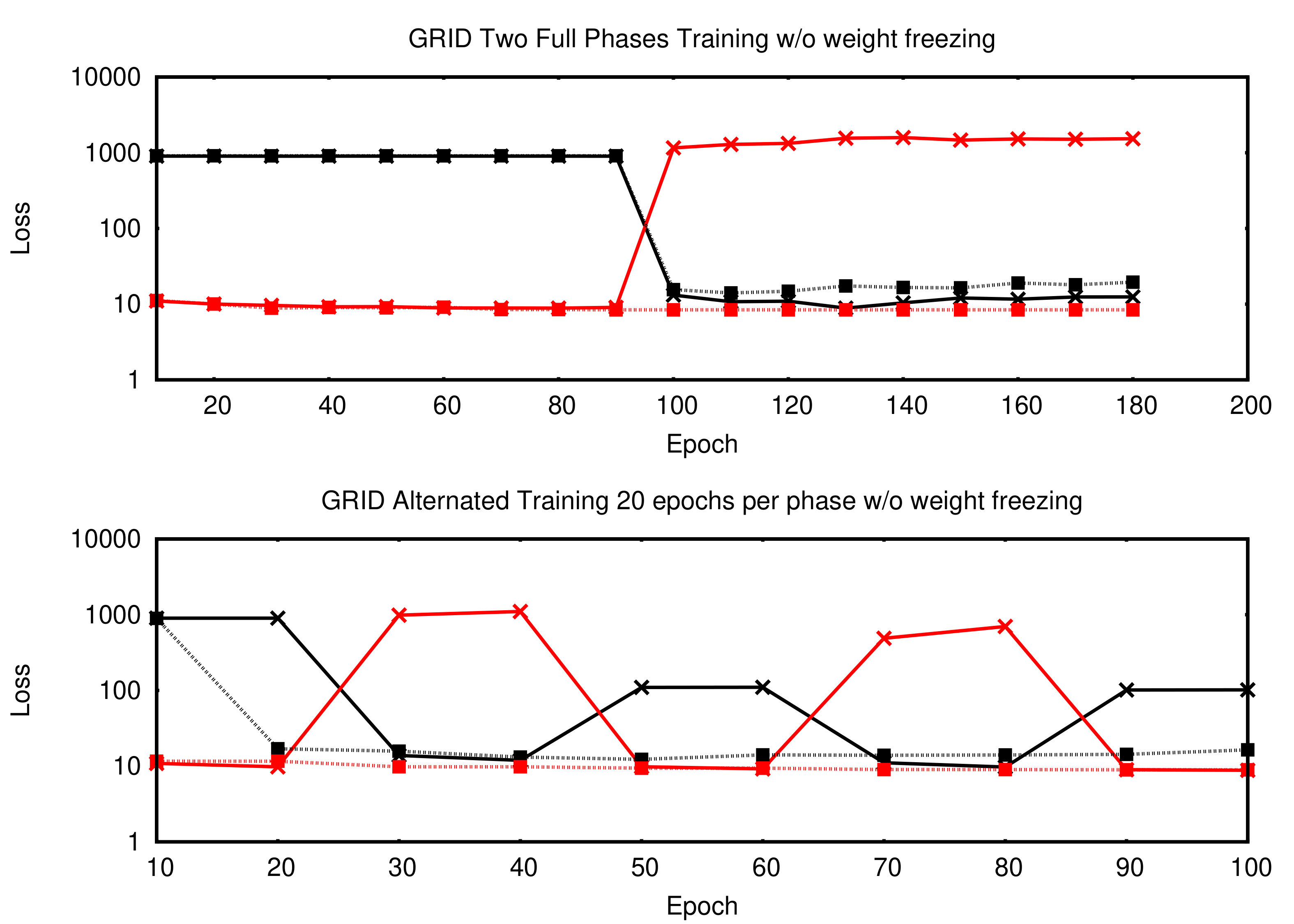 Figure 2
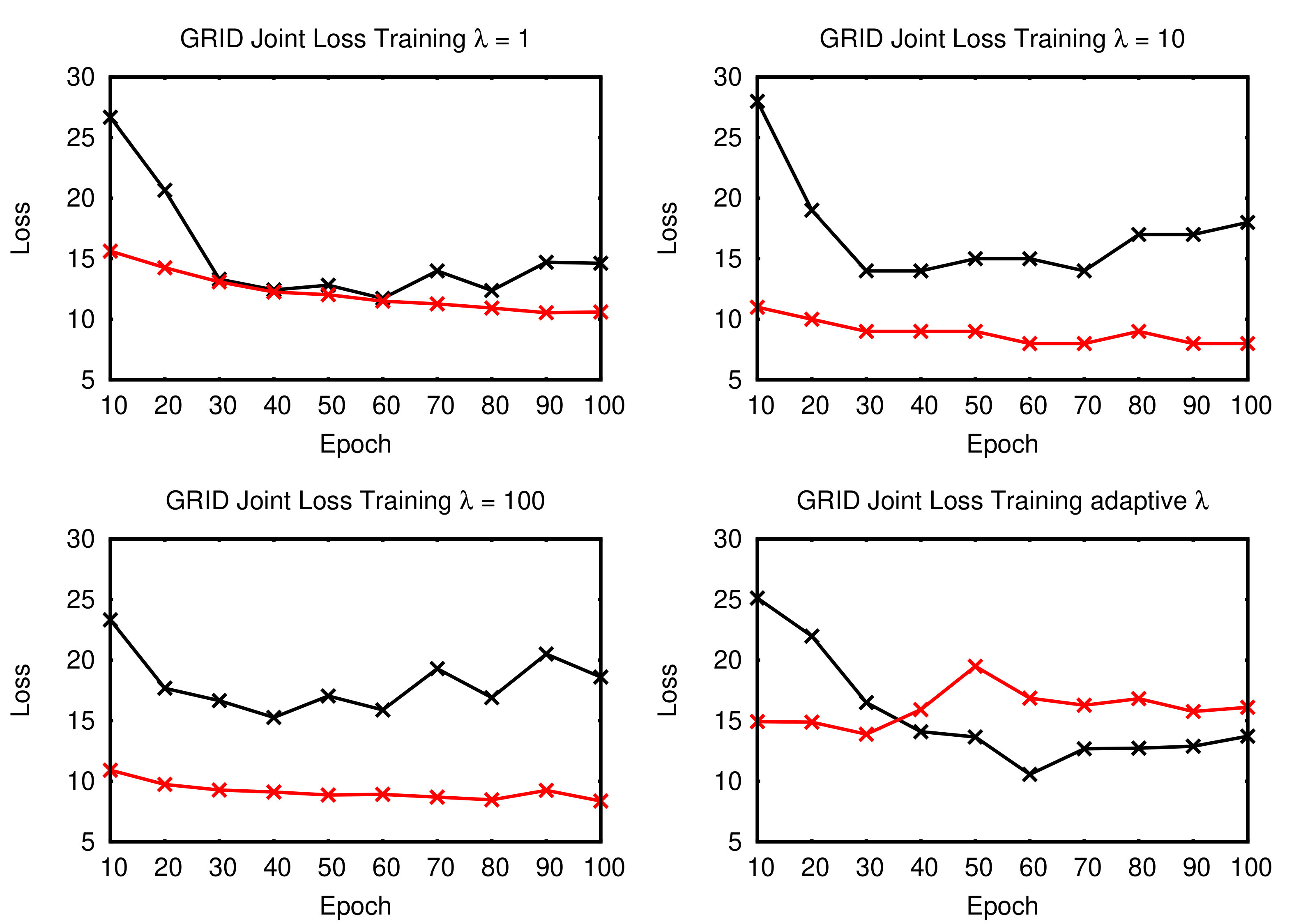 Figure 3
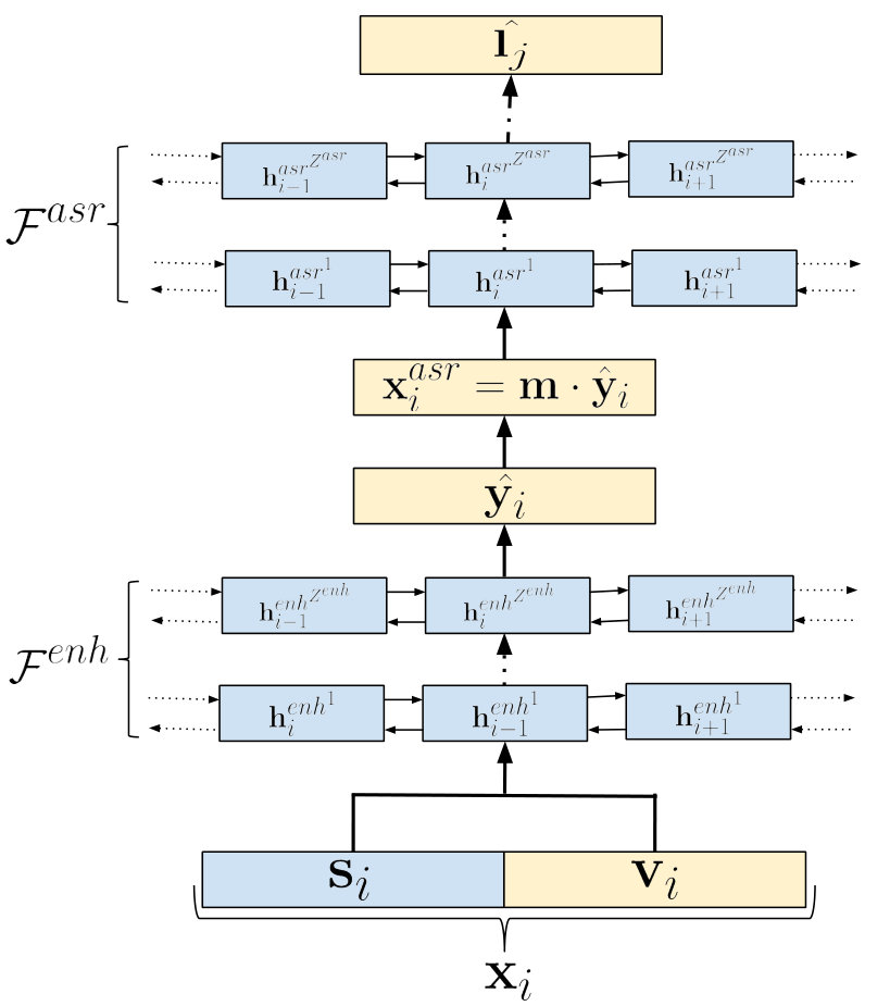 Figure 4
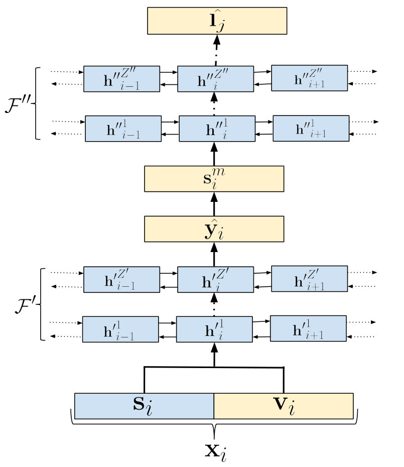 Figure 5
 Figure 6
 Figure 7
| GRID | TCD-TIMIT | ||
|---|---|---|---|
| Training Method | PER | PER-61 | PER-39 |
| ASR-Mod. Clean-Audio | |||
| ASR-Mod. Mixed-Audio | |||
| ASR-Mod. Mixed-A/V | |||
| ASR-Mod. Visual | |||
| Joint-Mod. Joint loss | |||
| Joint-Mod. Alt. 2 full | |||
| Joint-Mod. Alt. 2 full freeze | |||
| Joint-Mod. Alt. | |||
| Joint-Mod. Alt. freeze | |||
| Joint-Mod. PIT Alt. | |||
Peer Reviews
No public reviews on file for this paper yet. If you reviewed it on a platform where reviews are public (OpenReview, ICLR, NeurIPS, ICML), you can paste yours below so the community can read it here.
Videos
No videos yet. Explain this paper in a talk, walkthrough, or lecture? Add one.
An Analysis of Speech Enhancement and Recognition Losses in Limited Resources Multi-talker Single Channel Audio-Visual ASR
Abstract
In this paper, we analyzed how audio-visual speech enhancement can help to perform the ASR task in a cocktail party scenario. Therefore we considered two simple end-to-end LSTM-based models that perform single-channel audio-visual speech enhancement and phone recognition respectively. Then, we studied how the two models interact, and how to train them jointly affects the final result.
We analyzed different training strategies that reveal some interesting and unexpected behaviors. The experiments show that during optimization of the ASR task the speech enhancement capability of the model significantly decreases and vice-versa. Nevertheless the joint optimization of the two tasks shows a remarkable drop of the Phone Error Rate (PER) compared to the audio-visual baseline models trained only to perform phone recognition. We analyzed the behaviors of the proposed models by using two limited-size datasets, and in particular we used the mixed-speech versions of GRID and TCD-TIMIT.
**Index Terms— ** speech recognition, speech enhancement, cocktail party, multi-task learning, audio-visual.
1 Introduction
Although state-of-the-art speech recognition systems have reached very high accuracy, their performance drops significantly when the signal is recorded in challenging conditions (e.g. mismatched noises, low SNR, reverberation, multiple voices). On the other hand, humans show a remarkable ability in recognizing speech in such conditions (cocktail party effect [1]).
Some robust ASR systems process the audio signal through a speech enhancement or separation stage before passing it to the recognizer [2]. An alternative approach is to train the ASR model in a multi-task fashion where speech enhancement/separation and recognition modules are concatenated and jointly trained [3, 4, 5].
Several recent works showed significant advancements in speech separation [6, 7, 8, 9] and target speaker extraction [10, 11] from mixed-speech mixtures.
These works proposed end-to-end models and training strategies that are exploited to perform multi-speaker [12, 13] and target speaker speech recognition [14].
The aim of the paper is to study how the speech enhancement task can help in recognizing the phonetic transcription of the utterance spoken by target speaker from single-channel audio of several people talking simultaneously. Note that this is an ill-posed problem in that many different hypotheses about what the target speaker says are consistent with the mixture signal. We addressed this problem by exploiting the visual information associated to the speaker of interest in order to extract her speech from input mixed-speech signal. In [15] we demonstrated that face landmark’s movements are very effective visual features for the enhancement task when the size of the training dataset is limited.
In the last few years many audio-visual approaches have shown remarkable results by using neural networks to solve speech-related tasks with different modalities of the speech signal. These include audio-visual speech recognition [16, 17], audio-visual speech enhancement [18, 19, 20] and audio-visual speech separation [21, 22, 23].
It is well know that simultaneously learning multiple related tasks from data can be more advantageous rather than learning these tasks independently [24]. The class of these methods belong to Multi-Task Learning (MTL) [25].
Several speech processing applications are tightly related, so MTL methods can improve performance and reduce generalization error. In particular, robust ASR models show better accuracy when they are trained with other tasks [3, 5, 26].
An MTL LSTM-based model is proposed in [5], where the cost function is the weighted sum of ASR and speech enhancement losses. Some of these methods differ from the most common MTL approaches, where the differentiation of tasks is made only in the last layers of the network. These methods are also referred to as “joint learning”.
We study how the speech enhancement and recognition tasks interact using an approach that belongs to this class of methods. The approach is equivalent to merging two different models with different loss functions: one to optimize the speech enhancement, and one for the phone recognition task. Our aim is to analyze the interaction between the ASR and enhancement tasks, and understand whether (and how) it is advantageous to train them jointly. For this reason, we firstly train and analyze a simple ASR model, then we study whether adding a preliminary speech enhancement stage helps in performing the ASR task. In order to analyze how the two tasks (and the respective loss functions) interact we propose three different training techniques that allow to unveil the strengths and the weaknesses of this approach. In particular we focused our attention on a very common audio-visual setting where the quantity of available data for training the model is limited.
2 Models Architecture
In this section we present the models used to analyze and study how speech enhancement and recognition tasks can be combined to perform phone recognition in a cocktail party scenario. In order to perform a fair analysis, we use very simple and common architectures based on deep Bi-directional Long Short-Term Memory (BLSTM) [27]. These models are fed with the sequence where and/or the sequence . represents a spectrogram of the mixed-speech audio input, is the number of frames of the spectrogram and v is the motion vector computed from the video face landmarks [28] of the speaker of interest.
2.1 ASR Model
The ASR model consists of a deep-BLSTM. It first computes the mel-scale filter bank representation derived from the spectrogram :
[TABLE]
where is the matrix that warps the spectrogram to the mel-filter banks representation.
We developed 3 different versions of this model that differ by the input used to perform the ASR task. The first version only uses acoustic features, therefore .
The second version uses both audio and visual features, thus:
The last version of the ASR models only fed with motions vector computed from face landmarks: .
All the models map to the phone label by using BLSTM layers. The output of the last BLSTM layer is linearly projected onto in order to use the CTC loss. This ASR model can be defined as follows: . Where is the set of parameters of the ASR model. The model uses a CTC loss function to optimize the phone recognition task: .
2.2 Enhancement Model
The Enhancement model is developed with the goal of denoising the speech of the speaker of interest given the mixed-speech input. The model input at time step is: The speech enhancement task target is where is a slice of the spectrogram of the clean utterance spoken by the speaker of interest. The enhancement model consists of BLSTM layers and a final layer that projects the output onto . This last layer uses sigmoid as activation function and, in order to obtain values in a scale comparable to the speech enhancement target, it multiplies the output by , where is a constant and is a vector that contains the standard deviations of each output feature. The enhancement model can be defined as a function: , where is the sigmoidal function and is the set of parameters of the model. As loss function the model uses the Mean Squared Error (MSE):
2.3 Joint Model
In order to evaluate whether and how speech enhancement can help in performing ASR in cocktail party scenario, we developed a model that is the combination of the Enhancement model and the ASR model: . Note that only the enhancement part of the model exploits the visual information, while the ASR part receives in input only the output of the audio enhancement module .
2.4 Training Strategies
Our aim is to explore and study the behaviors of the two losses and . Therefore, we explored different techniques to perform training in order to analyze how the two losses interact.
The first training technique, henceforth referred to as joint loss, consists of using a loss that is a weighted sum of the two loss functions, ,
where is the coefficient that multiplies .
During training we observed that the ratio of the two losses significantly changes. To keep both the two losses at the same level of magnitude we also experimented with an adaptive coefficient
[TABLE]
The second training method, alternated training, consists of alternation of the speech enhancement and ASR training phases. This training procedure performs a few steps of each phase several times. The speech enhancement phase will use as loss function and therefore only parameters will be updated during this phase. During the ASR phase the loss function will be . A particular case of the alternated training is the alternated two full phases training where the two phases are performed only one time each for a large number of epochs.
In alternated training and alternated two full phases training, the optimization phase updates both and parameters. For both techniques we also developed a weight freezing version that optimize by only updating .
3 Experimental Setup
In this section, we report and discuss all the results obtained during the analysis.
3.1 Dataset
We decided to focus our analysis on a challenging and common scenario where the quantity of available data and resources is limited. Indeed, we performed the analysis by using the GRID [29] and TCD-TIMIT [30] audio-visual limited-size datasets. We used the mixed-speech speaker-independent versions of these two datasets proposed in [15] as a starting point and then added the phone transcriptions for the speaker of interest. The GRID and TCD-TIMIT dataset were respectively split into disjoint sets of // and // speakers for training/validation/testing respectively.
For both datasets we used standard TIMIT phone dictionary. In particular in GRID the number of used phones is limited to 33 (as the vocabulary is limited to few tens of words), while in TCD-TIMIT all the 61 TIMIT phones are present. Similarly to what is usually done with TIMIT, the 61 phones were mapped to 39 phones after decoding, when computing the Phone Error Rate (PER).
3.2 Baseline and Model Setup
In order to create a strong baseline to evaluate the performance of the joint model, we tested the various versions of the ASR model. All these baseline models consist of 2 layers of 250 hidden units and were trained by using back-propagation through time (BPTT) with Adam optimizer. For what concerns the joint model, we used the same number of layers for both ASR and enhancement components: . Each layer consists of 250 hidden units with activation function. We performed a limited random search-based hyper-parameter tuning, therefore all reported results may be slightly improved.
3.3 Phone Error Rate Evaluation
Table 1 reports PER of all baseline models and of the joint models with different training strategies. Note that the results on GRID obtained by using visual input can not be compared with the results obtained in [31] since our model was trained with a significantly smaller version of the dataset.
It is also important to point out that in the ASR-Model fed with Mixed-Audio/Video input the visual information does not help to reach better results, while in [15] we show that the visual information is very effective in performing speech enhancement.
The joint model achieved on TCD-TIMIT a PER that is comparable with the clean-audio baseline, while results on GRID are slightly worse but still much better than baseline results. Note that the difference in the achieved PER between the two datasets is mainly due to the difference of vocabulary size (GRID has a tiny 52 word vocabulary), phonotactics (as in GRID the word sequences are more constrained) and utterance lengths, indeed, the length of the sequences is variable in TCD-TIMIT, while it is fixed in GRID.
In both datasets, the joint model significantly outperforms baselines with mixed-speech input. In particular, the alternated training reaches better results in GRID while in TCD-TIMIT it is slightly outperformed by the alternated two full phases training with weight freezing. We evaluated the joint model also by substituting the loss by an MSE-based loss function trained by removing visual input information and by using permutation invariant training (PIT) optimization [8], a very effective audio-only technique. We reported the results in the last row of the Table 1 and in Figure 3 that show PIT performs worse than audio-visual counterparts.
3.4 Result Analysis
In this section, we analyze the trends of and during training, and in particular, we focus on their ratio. Due to space limitations, we only report, the loss curves computed on the GRID validation set, Figures 1, 2 and 3. However, we observed an analogous behavior on TCD-TIMIT.
The first method that we analyze is the alternated two full phases training. It first updates parameters to minimize the loss, until it reaches a plateau in terms of speech enhancement on the validation set.
Figure 1 shows that the alternated two full phases strategy from epoch 90, when the minimization of starts (and involves both and ) the speech enhancement loss function remarkably diverges in few epochs. This behavior suggests that the de-noised representation is not optimal to perform the phone recognition task, as observed in previous works [3, 4, 5], although we did not expect to observe such a strong divergence. The and curves obtained by using alternated two full phases training with weight freezing unveil another effect of this issue. Here parameters are forced to not change during the ASR training phase, and hence does not diverge but at the same time does not reach results as good as in the previous case. Figure 1 shows a similar behaviour of alternate training when weight freezing is applied.
The dramatic drop of the enhancement performance drove us to explore how the two losses evolve if they are trained together by using a joint loss method. Figure 2 shows the trends of and when using different fixed values of and the adaptive of equation 2. In this case while decreases, (after a certain point) tends to increase. For higher values of the gap between the two loss functions increases, indeed tends to diverge rapidly during training. The best result for is obtained using the adaptive value (also for TCD-TIMIT). The enhancement capability continually grows as the epochs pass, while PER optimization has a substantial slowdown after 40 epochs. This deceleration coincides with the start of the faster decrease of the enhancement loss. The joint loss training shows the interesting property of obtaining fair good results for both the metrics, but, in terms of ASR capability (that is the main goal of the model) the results turn out to be lower than the ones obtained with the some other training methods.
Figure 3 shows the trends of the two losses during alternated training, with different number of epochs per phase. Even in this case the decrease of coincides with a large increase of the value of and vice-versa. Moreover, every repetition of the two phases leads to a smaller gap between the two loss functions.
4 Conclusion
In this paper we studied how audio-visual single channel speech enhancement can help speech recognition when several people are talking simultaneously. The analysis unveils that jointly minimizing the speech enhancement loss and the CTC loss may not the best strategy to improve ASR. Then we explored the trends of the loss functions when the training strategy consists of an alternation of the speech enhancement and ASR training phases.We observed that the loss function that was not considered for the training phase tends to diverge. Finally, we found that the interaction between the two loss functions can be exploited in order to obtain better results. In particular, the alternated training method shows that PER can be gradually reduced by wisely alternating the two training phases.
The reference list from the paper itself. Each links out to its DOI / PubMed record.
- 1[1] Josh H Mc Dermott, “The cocktail party problem,” Current Biology , vol. 19, no. 22, pp. R 1024–R 1027, 2009.
- 2[2] Arun Narayanan and De Liang Wang, “Investigation of speech separation as a front-end for noise robust speech recognition,” IEEE/ACM Transactions on Audio, Speech, and Language Processing , vol. 22, no. 4, pp. 826–835, 2014.
- 3[3] Zhong-Qiu Wang and De Liang Wang, “Joint training of speech separation, filterbank and acoustic model for robust automatic speech recognition,” in Interspeech , 2015.
- 4[4] Arun Narayanan and De Liang Wang, “Improving robustness of deep neural network acoustic models via speech separation and joint adaptive training,” IEEE/ACM transactions on audio, speech, and language processing , vol. 23, no. 1, pp. 92–101, 2015.
- 5[5] Zhuo Chen, Shinji Watanabe, Hakan Erdogan, and John R Hershey, “Speech enhancement and recognition using multi-task learning of long short-term memory recurrent neural networks,” in Interspeech , 2015.
- 6[6] Z. Chen, Y. Luo, and N. Mesgarani, “Deep attractor network for single-microphone speaker separation,” in 2017 IEEE International Conference on Acoustics, Speech and Signal Processing (ICASSP) , March 2017, pp. 246–250.
- 7[7] Yusuf Isik, Jonathan Le Roux, Zhuo Chen, Shinji Watanabe, and John R. Hershey, “Single-channel multi-speaker separation using deep clustering,” in Interspeech , 2016.
- 8[8] Morten Kolbaek, Dong Yu, Zheng-Hua Tan, and Jesper Jensen, “Multitalker speech separation with utterance-level permutation invariant training of deep recurrent neural networks,” IEEE/ACM Trans. Audio, Speech and Lang. Proc. , vol. 25, no. 10, pp. 1901–1913, Oct. 2017.