TL;DR
This paper reviews and compares methods for effectively estimating deep variational auto-encoders in language modeling, addressing the challenge of posterior collapse with new techniques and practical recommendations.
Contribution
It provides a comprehensive survey, introduces novel techniques, and offers empirical insights and best practices for training deep probabilistic language models.
Findings
Many techniques perform similarly given sufficient resources
A convenient technique can be preferred for practical use
Empirical observations guide best practices in model estimation
Abstract
Advances in variational inference enable parameterisation of probabilistic models by deep neural networks. This combines the statistical transparency of the probabilistic modelling framework with the representational power of deep learning. Yet, due to a problem known as posterior collapse, it is difficult to estimate such models in the context of language modelling effectively. We concentrate on one such model, the variational auto-encoder, which we argue is an important building block in hierarchical probabilistic models of language. This paper contributes a sober view of the problem, a survey of techniques to address it, novel techniques, and extensions to the model. To establish a ranking of techniques, we perform a systematic comparison using Bayesian optimisation and find that many techniques perform reasonably similar, given enough resources. Still, a favourite can be named based…
Click any figure to enlarge with its caption.
 Figure 1
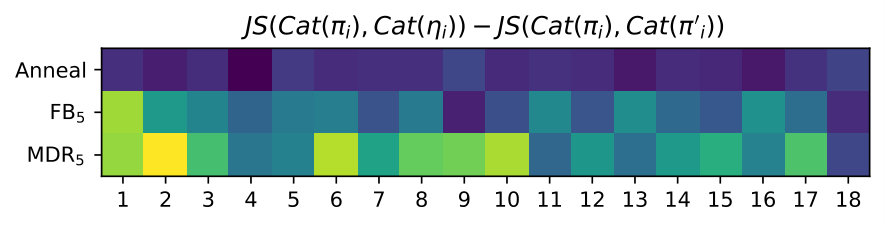 Figure 2
 Figure 3
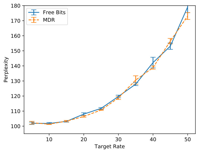 Figure 4
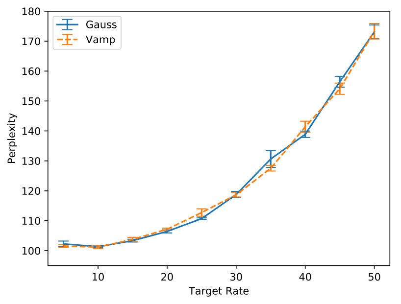 Figure 5
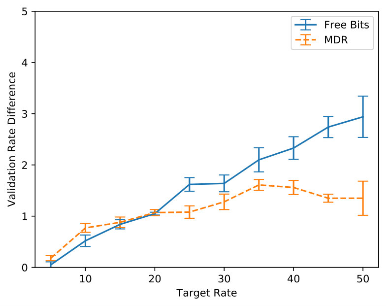 Figure 6
 Figure 7
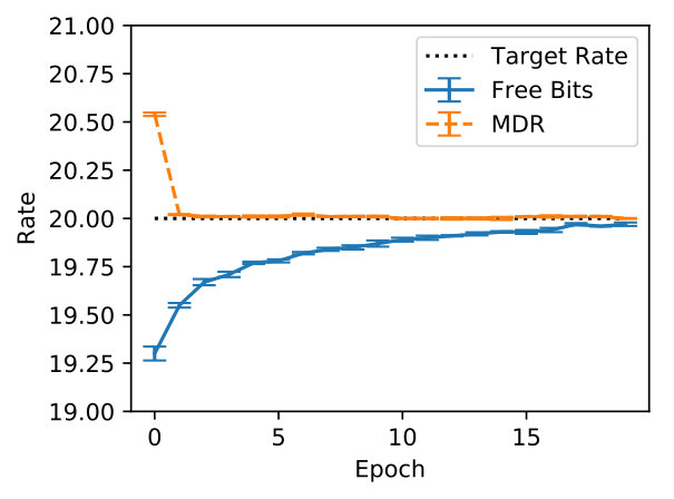 Figure 8
 Figure 9
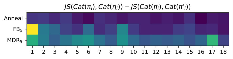 Figure 10
 Figure 11
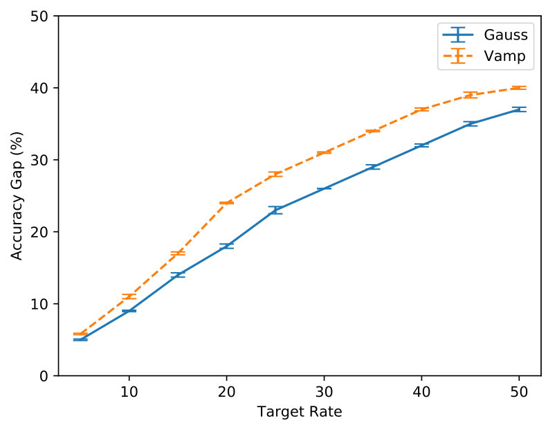 Figure 12
 Figure 13
 Figure 14
 Figure 15
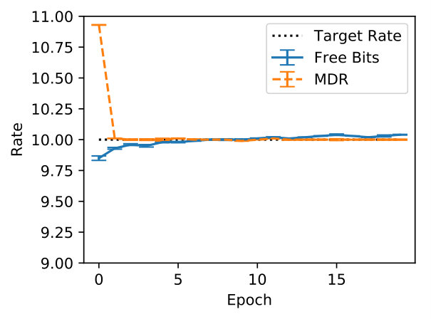 Figure 16
 Figure 17
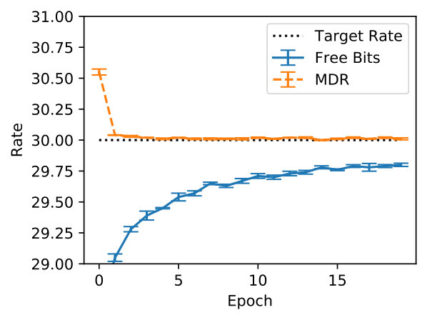 Figure 18
| Technique | Hyperparameters |
|---|---|
| KL annealing | increment () |
| Word dropout (WD) | decrement () |
| FB and MDR | target rate () |
| SFB | (), (), (), () |
| -VAE | KL weight () |
| InfoVAE | (), () |
| LagVAE | (), target MMD () |
| target -ELBO () |
| Mode | PPL | AU | Acc | ||||
|---|---|---|---|---|---|---|---|
| RnnLM | - | - | 107.10.5 | - | - | ||
| Vanilla | 118.4 | 0.0 | 105.70.4 | 0 | 0.0 | ||
| Annealing | 115.3 | 3.3 | 103.70.3 | 17 | 6.0 | ||
| WD | 117.6 | 0.0 | 102.50.6 | 0 | 0.0 | ||
| FB | 113.3 | 5.0 | 101.90.8 | 14 | 5.8 | ||
| SFB | 112.0 | 6.4 | 101.00.5 | 18 | 7.0 | ||
| MDR | 113.5 | 5.0 | 102.10.5 | 13 | 6.2 | ||
| -VAE | 113.0 | 5.3 | 101.70.5 | 11 | 6.1 | ||
| InfoVAE | 113.5 | 4.3 | 100.80.4 | 10 | 5.2 | ||
| LagVAE | 112.1 | 6.5 | 101.60.7 | 24 | 6.9 |
| Model | PPL | AU | Acc | |||
|---|---|---|---|---|---|---|
| RnnLM | - | - | 84.5 0.5 | - | - | |
| / | 103.5 | 5.0 | 81.5 0.5 | 13 | 5.4 | |
| MoG/ | 103.3 | 5.0 | 81.4 0.5 | 32 | 5.8 | |
| Vamp/ | 103.1 | 5.0 | 81.2 0.4 | 22 | 5.8 |
| Yahoo | Yelp | ||||||||
| Model | NLL | PPL | AU | NLL | PPL | AU | |||
| RnnLM | - | - | - | - | - | - | |||
| Lagging | - | - | |||||||
| -VAE () | - | - | |||||||
| Annealing | - | - | |||||||
| Vanilla | |||||||||
| / | |||||||||
| MoG/ | |||||||||
| Parameter | Value |
|---|---|
| Optimizer | Adam |
| Optimizer Parameters | |
| Learning Rate | 0.001 |
| Batch Size | 64 |
| Decoder Dropout Rate () | 0.4 |
| Weight Decay | |
| Maximum Sentence Length | 59 |
| Maximum Gradient Norm | 1.5 |
| Model | Parameter | Value |
|---|---|---|
| A | embedding units () | 256 |
| A | vocabulary size () | 25643 |
| R and S | decoder layers () | 2 |
| R and S | decoder hidden units () | 256 |
| S | encoder hidden units () | 256 |
| S | encoder layers () | 1 |
| S | latent units () | 32 |
| MoG | mixture components () | 100 |
| VampPrior | pseudo inputs () | 100 |
| Model | PPL | PPL |
|---|---|---|
| Dyer et al. (2016) | ||
| RnnLM | 84.5 0.52 |
| Parameter | Value |
|---|---|
| Objective Function | Validation NLL |
| Kernel | Matern52 |
| Acquisition Function | Expected Improvement |
| Parameter Inference | MCMC |
| MCMC Samples | 10 |
| Leapfrog Steps | 20 |
| Burn-in Samples | 100 |
Peer Reviews
No public reviews on file for this paper yet. If you reviewed it on a platform where reviews are public (OpenReview, ICLR, NeurIPS, ICML), you can paste yours below so the community can read it here.
Code & Models
Videos
No videos yet. Explain this paper in a talk, walkthrough, or lecture? Add one.
Effective Estimation of Deep Generative Language Models
Tom Pelsmaeker
ILCC
University of Edinburgh
&Wilker Aziz
ILLC
University of Amsterdam
[email protected] Work done while the first author was at the University of Amsterdam. Code is available at https://github.com/tom-pelsmaeker/deep-generative-lm
Abstract
Advances in variational inference enable parameterisation of probabilistic models by deep neural networks. This combines the statistical transparency of the probabilistic modelling framework with the representational power of deep learning. Yet, due to a problem known as posterior collapse, it is difficult to estimate such models in the context of language modelling effectively. We concentrate on one such model, the variational auto-encoder, which we argue is an important building block in hierarchical probabilistic models of language. This paper contributes a sober view of the problem, a survey of techniques to address it, novel techniques, and extensions to the model. To establish a ranking of techniques, we perform a systematic comparison using Bayesian optimisation and find that many techniques perform reasonably similar, given enough resources. Still, a favourite can be named based on convenience. We also make several empirical observations and recommendations of best practices that should help researchers interested in this exciting field.
1 Introduction
Deep generative models (DGMs) are probabilistic latent variable models parameterised by neural networks (NNs). Specifically, DGMs optimised with amortised variational inference and reparameterised gradient estimates (Kingma and Welling, 2014; Rezende et al., 2014), better known as variational auto-encoders (VAEs), have spurred much interest in various domains, including computer vision and natural language processing (NLP).
In NLP, VAEs have been developed for word representation (Rios et al., 2018), morphological analysis (Zhou and Neubig, 2017), syntactic and semantic parsing (Corro and Titov, 2018; Lyu and Titov, 2018), document modelling (Miao et al., 2016), summarisation (Miao and Blunsom, 2016), machine translation (Zhang et al., 2016; Schulz et al., 2018; Eikema and Aziz, 2019), language and vision (Pu et al., 2016; Wang et al., 2017), dialogue modelling (Wen et al., 2017; Serban et al., 2017), speech modelling (Fraccaro et al., 2016), and, of course, language modelling (Bowman et al., 2016; Goyal et al., 2017). One problem remains common to the majority of these models, VAEs often learn to ignore the latent variables.
We investigate this problem, dubbed posterior collapse, in the context of language models (LMs). In a deep generative LM (Bowman et al., 2016), sentences are generated conditioned on samples from a continuous latent space, an idea with various practical applications. For example, one can constrain this latent space to promote generalisations that are in line with linguistic knowledge and intuition (Xu and Durrett, 2018). This also allows for greater flexibility in how the model is used, for example, to generate sentences that live—in latent space—in a neighbourhood of a given observation (Bowman et al., 2016). Despite this potential, VAEs that employ strong generators (e.g. recurrent NNs) tend to ignore the latent variable. Figure 1 illustrates this point: neighbourhood in latent space does not correlate to patterns in data space, and the model behaves just like a standard LM.
Recently, many techniques have been proposed to address this problem (§3 and §7) and they range from modifications to the objective to changes to the actual model. Some of these techniques have only been tested under different conditions and under different evaluation criteria, and some of them have only been tested outside NLP. This paper contributes: (1) a novel strategy based on constrained optimisation towards a pre-specified upper-bound on mutual information; (2) multimodal priors that by design promote increased mutual information between data and latent code; last and, arguably most importantly, (3) a systematic comparison—in terms of resources dedicated to hyperparameter search and sensitivity to initial conditions—of strategies to counter posterior collapse, including some never tested for language models (e.g. InfoVAE, LagVAE, soft free-bits, and multimodal priors).
2 Density Estimation for Text
Density estimation for written text has a long history (Jelinek, 1980; Goodman, 2001), but in this work we concentrate on neural network models (Bengio et al., 2003), in particular, autoregressive ones (Mikolov et al., 2010). Following common practice, we model sentences independently, each a sequence of tokens.
2.1 Language models
A language model (LM) prescribes the generation of a sentence as a sequence of categorical draws parameterised in context, i.e.
[TABLE]
To condition on all of the available context, a fixed NN maps from a prefix sequence (denoted ) to the parameters of a categorical distribution over the vocabulary. We estimate the parameters of the model by searching for a local optimum of the log-likelihood function via stochastic gradient-based optimisation (Robbins and Monro, 1951; Bottou and Cun, 2004), where the expectation is taken w.r.t. the true data distribution and approximated with samples from a data set of i.i.d. observations. Throughout, we refer to this model as RnnLM alluding to a particular choice of that employs a recurrent neural network (Mikolov et al., 2010).
2.2 Deep generative language models
Bowman et al. (2016) model observations as draws from the marginal of a DGM. An NN maps from a latent sentence embedding to a distribution over sentences,
[TABLE]
where follows a standard Gaussian prior.111We use uppercase for probability mass functions and lowercase for probability density functions. Generation still happens one word at a time without Markov assumptions, but now conditions on in addition to the observed prefix. The conditional is commonly referred to as generator or decoder. The quantity is the marginal likelihood, essential for parameter estimation.
This model is trained to assign a high (marginal) probability to observations, much like standard LMs. Unlike standard LMs, it employs a latent space which can accommodate a low-dimensional manifold where discrete sentences are mapped to, via posterior inference , and from, via generation . This gives the model an explicit mechanism to exploit neighbourhood and smoothness in latent space to capture regularities in data space. For example, it may group sentences according to latent factors (e.g. lexical choices, syntactic complexity, etc.). It also gives users a mechanism to steer generation towards a specific purpose. For example, one may be interested in generating sentences that are mapped from the neighbourhood of another in latent space. To the extent this embedding space captures appreciable regularities, interest in this property is heightened.
Approximate inference
Marginal inference for this model is intractable and calls for variational inference (VI; Jordan et al., 1999), whereby an auxiliary and independently parameterised model approximates the true posterior . When this inference model is itself parameterised by a neural network, we have a case of amortised inference (Kingma and Welling, 2014; Rezende et al., 2014) and an instance of what is known as a VAE. Bowman et al. (2016) approach posterior inference with a Gaussian model
[TABLE]
whose parameters, i.e. a location vector and a scale vector , are predicted by a neural network architecture from an encoding of the complete observation .222We use boldface for deterministic vectors and for elementwise multiplication. In this work, we use a bidirectional recurrent encoder. Throughout the text we will refer to this model as SenVAE.
Parameter estimation
We can jointly estimate the parameters of both models (i.e. generative and inference) by locally maximising a lower-bound on the log-likelihood function (ELBO)
[TABLE]
For as long as we can reparameterise samples from using a fixed random source, automatic differentiation (Baydin et al., 2018) can be used to obtain unbiased gradient estimates of the ELBO (Kingma and Welling, 2014; Rezende et al., 2014).
3 Posterior Collapse
In VI, we make inferences using an approximation to the true posterior and choose as to minimise the KL divergence . The same principle yields a lower-bound on log-likelihood used to estimate jointly with , thus making the true posterior a moving target. If the estimated conditional can be made independent of , which in our case means relying exclusively on to predict the distribution of , the true posterior will be independent of the data and equal to the prior.333This follows trivially from the definition of posterior: . Based on such observation, Chen et al. (2017) argue that information that can be modelled by the generator without using latent variables will be modelled that way—precisely because when no information is encoded in the latent variable the true posterior equals the prior and it is then trivial to reduce to [math]. This is typically diagnosed by noting that after training for most : we say that the true posterior collapses to the prior. Alemi et al. (2018) show that the rate, , is an upperbound to , the mutual information (MI) between and . Thus, if is close to zero for most training instances, MI is either [math] or negligible. They also show that the distortion, , relates to a lower-bound on MI (the lower-bound being , where is the unknown data entropy).
A generator that makes no Markov assumptions, such as a recurrent LM, can potentially achieve , and indeed many have noticed that VAEs whose observation models are parameterised by such strong generators (or strong decoders) tend to ignore the latent representation (Bowman et al., 2016; Higgins et al., 2017; Sønderby et al., 2016; Zhao et al., 2018b). For this reason, a strategy to prevent posterior collapse is to weaken the decoder (Yang et al., 2017; Semeniuta et al., 2017; Park et al., 2018). In this work, we are interested in employing strong generators, thus we do not investigate weaker decoders. Other strategies involve changes to the optimisation procedure and manipulations to the objective that target local optima of the ELBO with non-negligible MI.
Annealing
Bowman et al. (2016) propose “KL annealing”, whereby the term in the is incorporated into the objective in gradual steps. This way the optimiser can focus on reducing distortion early on in training, potentially by increasing MI. They also propose to drop words from at random to weaken the decoder—intuitively the model would have to rely on to compensate for missing history. We experiment with a slight modification of word dropout whereby we slowly vary the dropout rate from . In a sense, we “anneal” from a weak to a strong generator.
Targeting rates
Another idea is to target a pre-specified rate (Alemi et al., 2018). Kingma et al. (2016) replace the term in the ELBO with , dubbed free bits (FB) because it allows encoding the first nats of information “for free”. As long as , this does not optimise a proper ELBO (it misses the term), and the introduces a discontinuity. Chen et al. (2017) propose soft free bits (SFB), that instead multiplies the term in the ELBO with a weighing factor that is dynamically adjusted based on the target rate : is incremented (or reduced) by if (or ). Note that this technique requires hyperparameters (i.e. ) besides to be tuned in order to determine how is updated.
Change of objective
We may also seek alternatives to the as an objective and relate them to quantities of interest such as MI. A simple adaptation of the ELBO weighs its KL-term by a constant factor (-VAE; Higgins et al., 2017). Setting promotes increased MI. Whilst being a useful counter to posterior collapse, low might lead to variational posteriors becoming point estimates. InfoVAE (Zhao et al., 2018b) mitigates this with a term aimed at minimising the divergence from the aggregated posterior to the prior. Following Zhao et al. (2018b), we approximate this with an estimate of maximum mean discrepancy (MMD; Gretton et al., 2012) in our experiments. Lagrangian VAE (LagVAE; Zhao et al., 2018a) casts VAE optimisation as a dual problem; it targets either maximisation or minimisation of (bounds on) under constraints on the InfoVAE objective. In MI-maximisation mode, LagVAE maximises a weighted lower-bound on MI, , under two constraints, a maximum -ELBO and a maximum MMD, that prevent from degenerating to a point mass. Reasonable values for these constraints have to be found empirically.
4 Minimum Desired Rate
We propose minimum desired rate (MDR), a technique to attain ELBO values at a pre-specified rate that does not suffer from the gradient discontinuities of FB, and does not introduce the additional hyperparameters of SFB. The idea is to optimise the ELBO subject to a minimum rate constraint :
[TABLE]
Because constrained optimisation is generally intractable, we optimise the Lagrangian (Boyd and Vandenberghe, 2004)
[TABLE]
where is a positive Lagrangian multiplier. We define the dual function and solve the dual problem . Local minima of the resulting min-max objective can be found by performing stochastic gradient descent with respect to and stochastic gradient ascent with respect to .
4.1 Relation to other techniques
It is insightful to compare MDR to the various techniques we surveyed in terms of the gradients involved in their optimisation. The losses minimised by annealing, -VAE, and SFB have the form , where . FB minimises the loss , where is the target rate. Last, with respect to and , MDR minimises the loss , where is the Lagrangian multiplier. And with respect to , MDR minimises .
[TABLE]
[TABLE]
5 Expressive Priors
Suppose we employ a multimodal prior , e.g. a mixture of Gaussians, and suppose we employ a unimodal posterior approximation, e.g. the typical diagonal Gaussian. This creates a mismatch between the prior and the posterior approximation families that makes it impossible for to be precisely [math]. For the aggregated posterior to match the prior, the inference model would have to—on average—cover all of the prior’s modes. Since the inference network is deterministic, it can only do so as a function of the conditioning input , thus increasing . Admittedly, this conditioning might still only capture shallow features of , and the generator may still choose to ignore the latent code, keeping low, but the potential seems to justify an attempt. This view builds upon Alemi et al. (2018)’s information-theoretic view which suggests that the prior regularises the inference model capping . Thus, we modify SenVAE to employ a more complex, ideally multimodal, parametric prior and fit its parameters.
MoG
Our first option is a uniform mixture of Gaussians (MoG), i.e.
[TABLE]
where the Gaussian parameters are optimised along with other generative parameters. Note that though we give this prior up to modes, the optimiser might merge some of them (by learning approximately the same location and scale).
VampPrior
Motivated by the fact that, for a fixed posterior approximation, the prior that optimises the equals , Tomczak and Welling (2018) propose the VampPrior, a variational mixture of posteriors:
[TABLE]
where is a learned pseudo input—in their case a continuous vector. Again the parameters of the prior, i.e. , are optimised in the ELBO. In our case, the input to the inference network is a discrete sentence, which is incompatible with the design of the VampPrior. Thus, we propose to bypass the inference network’s embedding layer and estimate a sequence of word embeddings, which makes up a pseudo input. That is, is a sequence where has the dimensionality of our embeddings, and is the length of the sequence (fixed at the beginning of training). Note, however, that for this prior to be multimodal, the inference model must already encode information in , thus there is some gambling in its design.
6 Experiments
Our goal is to identify which techniques are effective in training VAEs for language modelling. Our evaluation concentrates on intrinsic metrics: negative log-likelihood (NLL), perplexity per token (PPL), rate (), distortion (), the number of active units (AU; Burda et al., 2015))555A latent unit (a single dimension of ) is denoted active when its variance with respect to is larger than 0.01. and gap in the accuracy of next word prediction (given gold prefixes) when decoding from a posterior sample versus decoding from a prior sample (Acc).
For VAE models, NLL (and thus PPL) can only be estimated. We use importance sampling (IS)
[TABLE]
with our trained approximate posterior as importance distribution (we use samples).
We first report on experiments using the English Penn Treebank (PTB; Marcus et al., 1993).666We report on Dyer et al. (2016)’s pre-processing, rather than Mikolov et al. (2010)’s. Whereas our findings are quantitatively similar, qualitative analysis based on generations are less interesting with Mikolov’s far too small vocabulary.
RnnLM
The baseline RnnLM generator is a building block for all of our SenVAEs, thus we validate its performance as a strong standalone generator. We highlight that it outperforms an external baseline that employs a comparable number of parameters (Dyer et al., 2016) and that this performance boost is mostly due to tying embeddings with the output layer.777Stronger RNN-based models can be designed (Melis et al., 2018), but those use vastly more parameters. Appendix A.1 presents the complete architecture and a comparison.
Bayesian optimisation
The techniques we compare are sensitive to one or more hyperparameters (see Table 1), which we tune using Bayesian optimisation (BO) towards minimising estimated NLL of the validation data. For each technique, we ran 25 iterations of BO, each iteration encompassing training a model to full convergence. This was sufficient for the hyperparameters of each technique to converge. See Appendix A.2 for details.
On optimisation strategies
First, we assess the effectiveness of techniques that aim at promoting local optima of SenVAE with better MI tradeoff. As for the architecture, the approximate posterior employs a bidirectional recurrent encoder, and the generator is essentially our RnnLM initialised with a learned projection of (complete specification in A.1). We train with Adam (Kingma and Ba, 2014) with default parameters and a learning rate of until convergence five times for each technique.
Results can be found in Table 2. First, note how the vanilla VAE (no special treatment) encodes no information in latent space (). Then note that all techniques converged to VAEs that attain better PPL than the RnnLM and vanilla VAE, and all but annealed word dropout did so at non-negligible rate. Notably, the two most popular techniques, word dropout and annealing, perform sub-par to the other techniques.888Though here we show annealed word dropout, to focus on techniques that do not weaken the generator, standard word dropout also converged to negligible rates. The techniques that work well at non-negligible rates can be separated into two groups: one based on a change of objective (i.e., -VAE, InfoVAE and LagVAE), another based on targeting a specific rate (i.e., FB, SFB, and MDR). InfoVAE, LagVAE and SFB all require tuning of multiple hyperparameters. InfoVAE and LagVAE, in particular, showed poor performance without this careful tuning. In the first group, consider LagVAE, for example. Though Zhao et al. (2018a) argue that the magnitude of is not particularly important (in MI-maximisation mode, they fixed it to ), we could not learn a useful SenVAE with LagVAE until we allowed BO to also estimate the magnitude of . Once BO converges to the values in Table 1, the method does perform quite well.
Generally, it is hard to believe that hyperparameters transfer across data sets, thus it is fair to expect that this exercise will have to be repeated every time. We argue that the rate hyperparameter common to the techniques in the second group is more interpretable and practical in most cases. For example, it is easy to grid-search against a handful of values. Hence, we further investigate FB and MDR by varying the target rate further (from to ). SFB is left out, for MDR generalises SFB’s handcrafted update rule. We observe that FB and MDR attain essentially the same PPL across rates, though MDR attains the desired rate earlier on in training, especially for higher targets (where FB fails at reaching the specified rate). Importantly, at the end of training, the validation rate is closer to the target for MDR. Appendix B supports these claims. Though Acc already suggests it, Figure 2 shows more visibly that MDR leads to output Categorical distributions that are more sensitive to the latent encoding. We measure this sensitivity in terms of symmetrised KL between output distributions obtained from a posterior sample and output distributions obtained from a prior sample for the same time step given an observed prefix.
On expressive priors
Second, we compare the impact of expressive priors. This time, prior hyperparameters were selected via grid search and can be found in Appendix A.1. All models are trained with a target rate of using MDR, with settings otherwise the same as the previous experiment. In Table 3 it can be seen that more expressive priors do not improve perplexity further,999Here we remark that best runs (based on validation performance) do show an advantage, which stresses the need to report multiple runs as we do. though they seem to encode more information in the latent variable—note the increased number of active units and the increased gap in accuracy. One may wonder whether stronger priors allow us to target higher rates without hurting PPL. This does not seem to be the case: as we increase rate to , all models perform roughly the same, and beyond performance degrades quickly.101010We also remark that, without MDR, the MoG model attains validation rate of about . The models did, however, show a further increase in active units (VampPrior) and accuracy gap (both priors). Again, Appendix B contains plots supporting these claims.
Generated samples
Figure 3 shows samples from a well-trained SenVAE, where we decode greedily from a prior sample—this way, all variability is due to the generator’s reliance on the latent sample. Recall that a vanilla VAE ignores and thus greedy generation from a prior sample is essentially deterministic in that case (see Figure 1(a)). Next to the samples we show the closest training instance, which we measure in terms of an edit distance (TER; Snover et al., 2006).111111This distance metric varies from [math] to , where indicates the sentence is completely novel and [math] indicates the sentence is essentially copied from the training data. This “nearest neighbour” helps us assess whether the generator is producing novel text or simply reproducing something it memorised from training. In Figure 4 we show a homotopy: here we decode greedily from points lying between a posterior sample conditioned on the first sentence and a posterior sample conditioned on the last sentence. In contrast to the vanilla VAE (Figure 1(b)), neighbourhood in latent space is now used to capture some regularities in data space. These samples add support to the quantitative evidence that our DGMs have been trained not to neglect the latent space. In Appendix B we provide more samples.
Other datasets
To address the generalisability of our claims to other, larger, datasets, we report results on the Yahoo and Yelp corpora Yang et al. (2017) in Table 4. We compare to the work of He et al. (2019), who proposed to mitigate posterior collapse with aggressive training of the inference network, optimising the inference network multiple steps for each step of the generative network.121212To enable direct comparison we replicated the experimental setup from He et al. (2019) and built our methods into their codebase.. We report on models trained with the standard prior as well as an MoG prior both optimised with MDR, and a model trained without optimisation techniques.131313We focus on MoG since the PTB experiments showed the VampPrior to underperform in terms of AU. It can be seen that MDR compares favourably to other optimisation techniques reported in He et al. (2019). Whilst aggressive training of the inference network performs slightly better in terms of NLL and leads to more active units, it slows down training by a factor of 4. The MoG prior improves results on Yahoo but not on Yelp. This may indicate that a multimodal prior does offer useful extra capacity to the latent space,141414We tracked the average KL divergence between any two components of the prior and observed that the prior remained multimodal. at the cost of more instability in optimisation. This confirms that targeting a pre-specified rate leads to VAEs that are not collapsed without hurting NLL.
Recommendations
We recommend targeting a specific rate via MDR instead of annealing (or word dropout). Besides being simple to implement, it is fast and straightforward to use: pick a rate by plotting validation performance against a handful of values. Stronger priors, on the other hand, while showing indicators of higher mutual information (e.g. AU and Acc), seem less effective than MDR. Use IS estimates of NLL, rather than single-sample ELBO estimates, for model selection, for the latter can be too loose of a bound and too heavily influenced by noisy estimates of KL.151515This point seems obvious to many, but enough published papers report exponentiated loss or distortion per token, which, besides unreliable, make comparisons across papers difficult. Use many samples for a tight bound.161616We use samples. Compared to a single sample estimate, we have observed differences up to perplexity points in non-collapsed models. From to samples, differences are in the order of suggesting our IS estimate is close to convergence. Inspect sentences greedily decoded from a prior (or posterior) sample as this shows whether the generator is at all sensitive to the latent code. Retrieve nearest neighbours to spot copying behaviour.
7 Related Work
In NLP, posterior collapse was probably first noticed by Bowman et al. (2016), who addressed it via word dropout and KL scaling. Further investigation revealed that in the presence of strong generators, the ELBO itself becomes the culprit (Chen et al., 2017; Alemi et al., 2018), as it lacks a preference regarding MI. Posterior collapse has also been ascribed to approximate inference (Kim et al., 2018; Dieng and Paisley, 2019). Beyond the techniques compared and developed in this work, other solutions have been proposed, including modifications to the generator (Semeniuta et al., 2017; Yang et al., 2017; Park et al., 2018; Dieng et al., 2019), side losses based on weak generators (Zhao et al., 2017), factorised likelihoods (Ziegler and Rush, 2019; Ma et al., 2019), cyclical annealing (Liu et al., 2019) and changes to the ELBO (Tolstikhin et al., 2018; Goyal et al., 2017).
Exploiting a mismatch in correlation between the prior and the approximate posterior, and thus forcing a lower-bound on the rate, is the principle behind -VAEs (Razavi et al., 2019) and hyperspherical VAEs (Xu and Durrett, 2018). The generative model of -VAEs has one latent variable per step of the sequence, i.e. , making it quite different from that of the SenVAEs considered here. Their mean-field inference model is a product of independent Gaussians, one per step, but they construct a correlated Gaussian prior by making the prior distribution over the next step depend linearly on the previous step, i.e. with hyperparameters and . Hyperspherical VAEs work on the unit hypersphere with a uniform prior and a non-uniform VonMises-Fisher posterior approximation (Davidson et al., 2018). Note that, though in this paper we focused on Gaussian (and mixture of Gaussians, e.g. MoG and VampPrior) priors, MDR is applicable for whatever choice of prescribed prior. Whether its benefits stack with the effects due to different priors remains an empirical question.
GECO (Rezende and Viola, 2018) casts VAE optimisation as a dual problem, and in that it is closely related to our MDR and the LagVAE. GECO targets minimisation of under constraints on distortion, whereas LagVAE targets either maximisation or minimisation of (bounds on) under constraints on the InfoVAE objective. Contrary to MDR, GECO focuses on latent space regularisation and offers no explicit mechanism to mitigate posterior collapse.
Recently Li et al. (2019) proposed to combine FB, KL scaling, and pre-training of the inference network’s encoder on an auto-encoding objective. Their techniques are complementary to ours in so far as their main finding—the mutual benefits of annealing, pre-training, and lower-bounding KL—is perfectly compatible with ours (MDR and multimodal priors).
8 Discussion
SenVAE is a deep generative model whose generative story is rather shallow, yet, due to its strong generator component, it is hard to make effective use of the extra knob it offers. In this paper, we have introduced and compared techniques for effective estimation of such a model. We show that many techniques in the literature perform reasonably similarly (i.e. FB, SFB, -VAE, InfoVAE), though they may require a considerable hyperparameter search (e.g. SFB and InfoVAE). Amongst these, our proposed optimisation subject to a minimum rate constraint is simple enough to tune (as FB it only takes a pre-specified rate and unlike FB it does not suffer from gradient discontinuities), superior to annealing and word dropout, and require less resources than strategies based on multiple annealing schedules and/or aggressive optimisation of the inference model. Other ways to lower-bound rate, such as by imposing a multimodal prior, though promising, still require a minimum desired rate.
The typical RnnLM is built upon an exact factorisation of the joint distribution, thus a well-trained architecture is hard to improve upon in terms of log-likelihood of gold-standard data. Our interest in latent variable models stems from the desire to obtain generative stories that are less opaque than that of an RnnLM, for example, in that they may expose knobs that we can use to control generation and a hierarchy of steps that may award a degree of interpretability to the model. The SenVAE is not that model, but it is a crucial building block in the pursue for hierarchical probabilistic models of language. We hope this work, i.e. the organised review it contributes and the techniques it introduces, will pave the way to deeper—in statistical hierarchy—generative models of language.
Acknowledgments
This project has received funding from the European Union’s Horizon 2020 research and innovation programme under grant agreement No 825299 (GoURMET).
Appendix A Architectures and Hyperparameters
In order to ensure that all our experiments are fully reproducible, this section provides an extensive overview of the model architectures, as well as model and optimisation hyperparameters.
Some hyperparameters are common to all experiments, e.g. optimiser and dropout, they can be found in Table 5. All models were optimised with Adam using default settings (Kingma and Ba, 2014). To regularise the models, we use dropout with a shared mask across time-steps (Zaremba et al., 2014) and weight decay proportional to the dropout rate (Gal and Ghahramani, 2015) on the input and output layers of the generative networks (i.e. RnnLM and the recurrent decoder in SenVAE). No dropout is applied to layers of the inference network as this does not lead to consistent empirical benefits and lacks a good theoretical basis. Gradient norms are clipped to prevent exploding gradients, and long sentences are truncated to three standard deviations above the average sentence length in the training data.
A.1 Architectures
This section describes the components that parameterise our models.171717All models were implemented with the PyTorch library (Paszke et al., 2017), using default modules for the recurrent networks, embedders and optimisers. We use mnemonic blocks to describe architectures. Table 6 lists hyperparameters for the models discussed in what follows.
RnnLM
At each step, an RnnLM parameterises a categorical distribution over the vocabulary, i.e. , where and
[TABLE]
We employ an embedding layer (), one (or more) cell(s) ( is a parameter of the model), and an layer to map from the dimensionality of the GRU to the vocabulary size. Table 7 compares our RnnLM to an external baseline with a comparable number of parameters.
Gaussian SenVAE
A Gaussian SenVAE also parameterises a categorical distribution over the vocabulary for each given prefix, but, in addition, it conditions on a latent embedding , i.e. where and
[TABLE]
Compared to RnnLM, we modify only slightly by initialising GRU cell(s) with computed as a learnt transformation of . Because the marginal of the Gaussian SenVAE is intractable, we train it via variational inference using an inference model where
[TABLE]
Note that we reuse the embedding layer from the generative model. Finally, a sample is obtained via where .
MoG prior
We parameterise diagonal Gaussians, which are mixed uniformly. To do so we need location vectors, each in , and scale vectors, each in . To ensure strict positivity for scales we make . The set of generative parameters is therefore extended with and , each in .
VampPrior
For this we estimate sequences of input vectors, each sequence corresponds to a pseudo-input. This means we extend the set of generative parameters with , each in , for . For each , we sample at the beginning of training and keep it fixed. Specifically, we drew samples from a normal, , which we rounded to the nearest integer. and are the dataset sentence length mean and variance respectively.
A.2 Bayesian optimisation
Bayesian optimisation (BO) is an efficient method to approximately search for global optima of a (typically expensive to compute) objective function , where is a vector containing the values of hyperparameters that may influence the outcome of the function (Snoek et al., 2012). Hence, it forms an alternative to grid search or random search (Bergstra and Bengio, 2012) for tuning the hyperparameters of a machine learning algorithm. BO works by assuming that our observations (for ) are drawn from a Gaussian process (GP; Rasmussen and Williams, 2005). Then based on the GP posterior, we can design and infer an acquisition function. This acquisition function can be used to determine where to “look next” in parameter-space, i.e. it can be used to draw for which we then evaluate the objective function . This procedure iterates until a set of optimal parameters is found with some level of confidence.
In practice, the efficiency of BO hinges on multiple choices, such as the specific form of the acquisition function, the covariance matrix (or kernel) of the GP and how the parameters of the acquisition function are estimated. Our objective function is the (importance-sampled) validation NLL, which can only be computed after a model convergences (via gradient-based optimisation of the ELBO). We follow the advice of Snoek et al. (2012) and use MCMC for estimating the parameters of the acquisition function. This reduced the amount of objective function evaluations, speeding up the overall search. Other settings were also based on results by Snoek et al. (2012), and we refer the interested reader to that paper for more information about BO in general. A summary of all relevant settings of BO can be found in Table 8. We used the GPyOpt library (authors, 2016) to implement this procedure.
Appendix B Additional Empirical Evidence
In Figure 5 we inspect how MDR and FB approach different target rates (namely, , , and ). Note how MDR does so more quickly, especially at higher rates. Figure 6(a) shows that in terms of validation perplexity, MDR and FB perform very similarly across target rates. However, Figure 6(b) shows that at the end of training the difference between the target rate and the validation rate is smaller for MDR.
Figure 7 compares variants of SenVAE trained with MDR for various rates: a Gaussian-posterior and Gaussian-prior (blue-solid) to a Gaussian-posterior and Vamp-prior (orange-dashed). They perform essentially the same in terms of perplexity (Figure 7(a)), but the variant with the stronger prior relies more on posterior samples for reconstruction (Figure 7(b)).
Finally, we list additional samples: Figure 8 lists samples from RnnLM, vanilla SenVAE and effectively trained variants (via MDR with target rate ); Figure 9 lists homotopies from SenVAE models.
The reference list from the paper itself. Each links out to its DOI / PubMed record.
- 1Alemi et al. (2018) Alexander Alemi, Ben Poole, Ian Fischer, Joshua Dillon, Rif A Saurous, and Kevin Murphy. 2018. Fixing a broken elbo. In International Conference on Machine Learning , pages 159–168.
- 2authors (2016) The G Py Opt authors. 2016. G Py Opt: A bayesian optimization framework in python. http://github.com/Sheffield ML/G Py Opt .
- 3Baydin et al. (2018) Atilim Gunes Baydin, Barak A Pearlmutter, Alexey Andreyevich Radul, and Jeffrey Mark Siskind. 2018. Automatic differentiation in machine learning: a survey. Journal of Marchine Learning Research , 18:1–43.
- 4Bengio et al. (2003) Yoshua Bengio, Réjean Ducharme, Pascal Vincent, and Christian Jauvin. 2003. A neural probabilistic language model. Journal of machine learning research , 3(Feb):1137–1155.
- 5Bergstra and Bengio (2012) James Bergstra and Yoshua Bengio. 2012. Random search for hyper-parameter optimization. Journal of Machine Learning Research , 13(Feb):281–305.
- 6Bottou and Cun (2004) Léon Bottou and Yann L. Cun. 2004. Large scale online learning. In S. Thrun, L. K. Saul, and B. Schölkopf, editors, Advances in Neural Information Processing Systems 16 , pages 217–224. MIT Press.
- 7Bowman et al. (2016) Samuel R Bowman, Luke Vilnis, Oriol Vinyals, Andrew Dai, Rafal Jozefowicz, and Samy Bengio. 2016. Generating sentences from a continuous space. In Proceedings of The 20th SIGNLL Conference on Computational Natural Language Learning , pages 10–21.
- 8Boyd and Vandenberghe (2004) Stephen Boyd and Lieven Vandenberghe. 2004. Convex optimization . Cambridge university press.