Non-Markovian evolution of multi-level system interacting with several reservoirs. Exact and approximate
A.E. Teretenkov

TL;DR
This paper presents an exactly solvable model for multi-level quantum systems interacting with multiple reservoirs at zero temperature, comparing exact and approximate decay and decoherence rates.
Contribution
It introduces a solvable model and systematically compares exact solutions with common approximate master equations for multi-reservoir interactions.
Findings
Exact and approximate rates are quantitatively compared.
Parameter space is classified based on discrepancies between exact and approximate rates.
Insights into the validity of approximate methods in different regimes.
Abstract
An exactly solvable model for the multi-level system interacting with several reservoirs at zero temperatures is presented. Population decay rates and decoherence rates predicted by exact solution and several approximate master equations, which are widespread in physical literature, are compared. The space of parameters is classified with respect to different inequities between the exact and approximate rates.
Click any figure to enlarge with its caption.
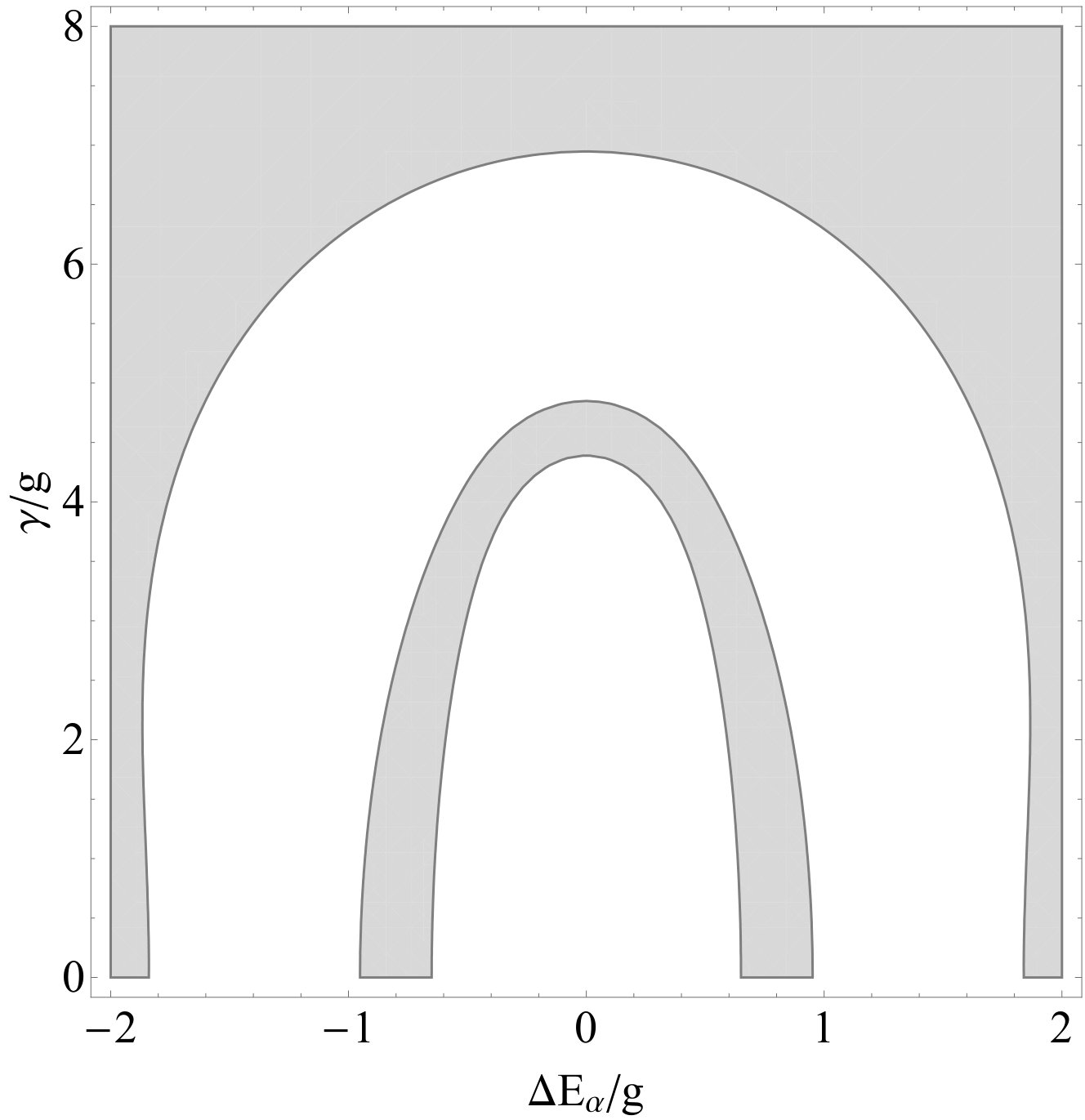 Figure 1
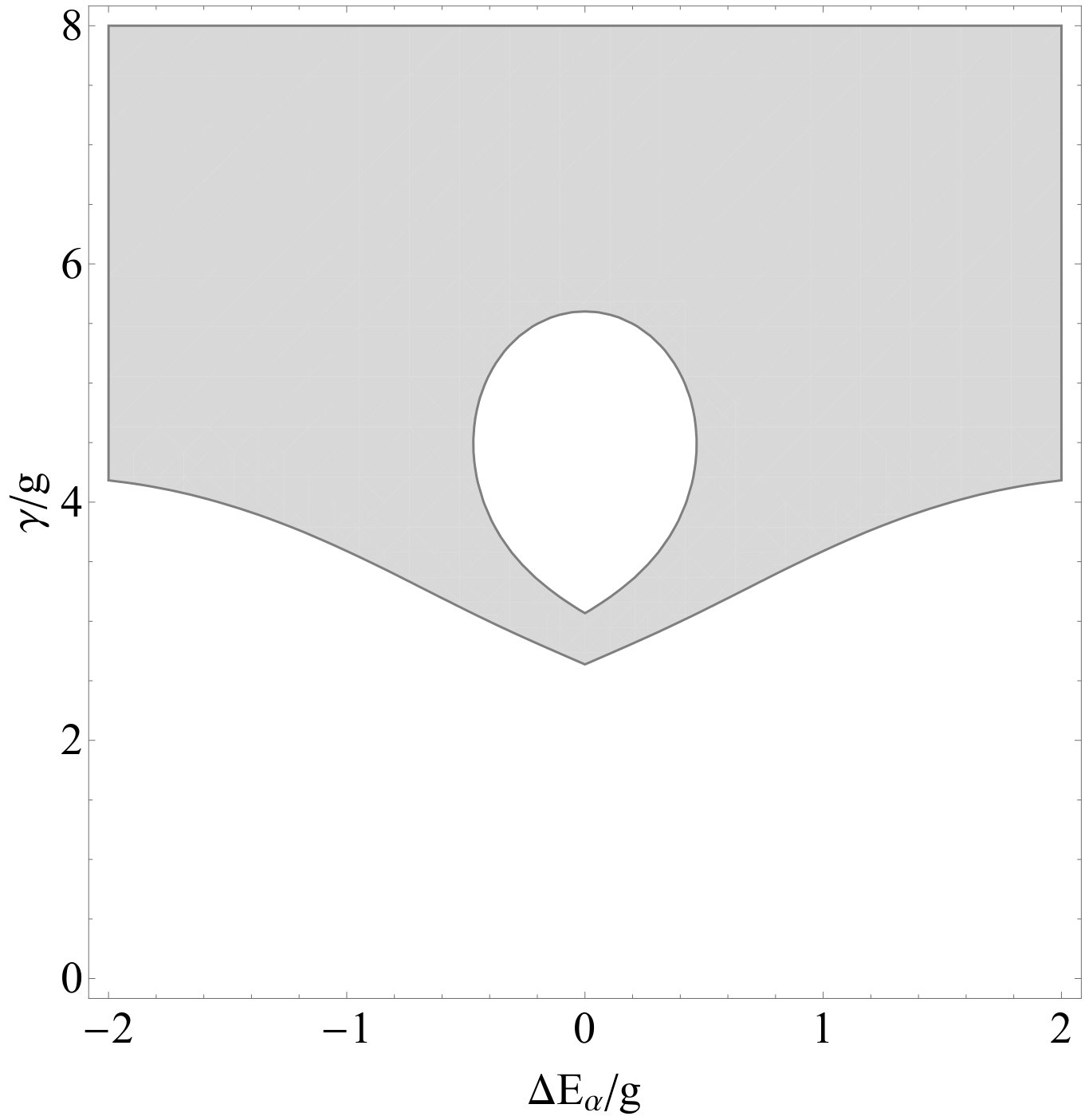 Figure 2
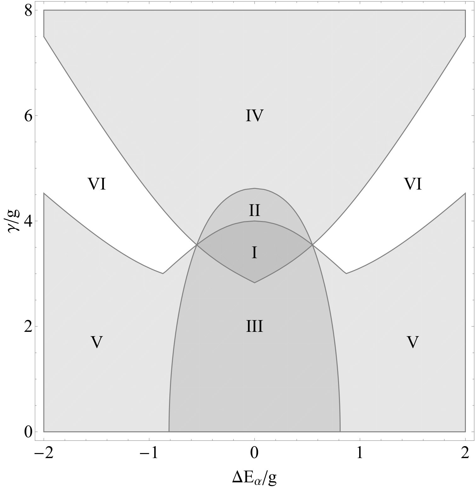 Figure 3
Peer Reviews
No public reviews on file for this paper yet. If you reviewed it on a platform where reviews are public (OpenReview, ICLR, NeurIPS, ICML), you can paste yours below so the community can read it here.
Videos
No videos yet. Explain this paper in a talk, walkthrough, or lecture? Add one.
Non-Markovian evolution of multi-level system interacting with several reservoirs. Exact and approximate111The research was supported by RSF (project No. 17-71-20154).
**A.E. Teretenkov222Steklov Mathematical Institute of Russian Academy of Sciences, ul. Gubkina 8, Moscow 119991, Russia; Lomonosov Moscow State University, Leninskie Gory 1, Moscow 119991, Russia
E-mail:[email protected]**
An exactly solvable model for the multi-level system interacting with several reservoirs at zero temperatures is presented. Population decay rates and decoherence rates predicted by exact solution and several approximate master equations, which are widespread in physical literature, are compared. The space of parameters is classified with respect to different inequities between the exact and approximate rates.
1 Introduction
In this work we consider the evolution of the multi-level system each level of which interacts with its own bosonic reservoir at zero temperature. For the simplicity we assume that the reservoirs are similar and the coupling of each level to its reservoir is also similar (the explicit mathematical model is described in Section 2). The main aim of the work is the comparison of the exact evolution of the reduced density matrix of the system (obtained by the pseudomode method, see Section 3) with the approximate evolution defined by master equations which are widespread in the physical literature. Namely, we consider the Nakajima-Zwanzig equation in the Born approximation, the non-Markovian Redfield equation and the Markovian Redfield equation. Usually in physical literature equations for the reduced density matrix are derived in the following way. The initial Liouville-von Neumann (linear differential) equation is reduced to the Nakajima-Zwanzig (linear integro-differential) equation [1, 2] (or some equivalent equation obtained by exclusion of reservoirs degrees of freedom). The Nakajima–Zwanzig is an exact equation for the reduced density matrix. Then the following four assumptions are subsequently done:
Born approximation [3, p. 131], [4, p. 7]. This equation is also integro-differential, which allows one to consider it as a non-Markovian one [5, 6]. Sometimes this approximation is also called the Redfield approximation or the second-order approximation [7, p. 249], [8, Subsec. 11.2], [9]. 2. 2.
Assumption that the reduced density matrix inside the integral could be taken at the same time as outside, which leads to the non-Markovian Redfield equation [10], [3, p. 132], [11]. Actually, this approximation is very close to Markovianity but only on the long times. 3. 3.
The full Markovian approximation, which leads to the Markovian Redfield equation [12, p. 141], [3, p. 132] , [4, p. 7], . 4. 4.
Secular approximation [3, p. 132], [12, p. 145], which leads to Markovian equations with the Gorini–Kossakowski–Sudarshan–Lindblad (GKSL) generator [14, 13].
At the same time only the equation which obtained after all four assumptions has mathematically strict justification [15, 16]. And its derivation goes back to [17, 18] and is based on the van Hove–Bogolyubov scaling [16, Sec. 1.8]. Moreover, only the last equation guarantees positivity and even complete positivity [14, 13]. At the same time the Redfield equation can violate the positivity, which indeed could be fixed by applying the slippage-operators to the initial conditions [19, 20, 21] or by some other methods [22]. On the other hand, in physical calculations the Redfield equation without secular approximation is frequently used [24, 23]. Some advantage of the Redfield equation in comparison with GKSL equations of the secular approximation are discussed in [25, 26]. For the damped oscillator the Redfield equation can both be translation invariant and have canonical equilibrium state [27] rather than GKSL equation [28]. If the aim is to take into account the non-Markovian effects then only Born approximation is usually done [9]. Thus, it is suggested in physical literature that the equations of the first one or two approximations could be more accurate than the GKSL equation which needs all four approximations. So it is natural to study the exactly solvable model to compare its prediction with the approximate ones.
In Section 2 we present the initial problem for the system and the reservoirs. It is important to mention that we introduce the Hamiltonian which is already in the rotating wave approximation form. Hence we leave the discussion of this approximation by itself out of the range of our study. At the same time, if one derives GKSL equations by the stochastic limit approach, then it is not necessary to assume this approximation and its a corollary of the van Hove–Bogolyubov scaling [16].
In Section 3 we present the pseudomode approach and obtain the exact evolution of the reduced density matrix. This approach was developed in [29, 30, 31, 32, 33, 34]. In [35] we have shown that the Friedrichs model [36] naturally arises as an intermediate step in this approach. In a quite general form the description of the non-Markovian evolution in the Friedrichs approximation was discussed in [37].
In Sections 4 and 5 we present the Nakajima-Zwanzig equation in Born approximation and the Redfield equation (both non-Markovian and Markovian) for our special case, accordingly, and solve them. In our case the Markovian Redfield equation appears to be identical to the one with the secular approximation.
Finally, in Section 6 we compare the solutions for exact and approximate equations. In Conclusions we summarize our results and suggest the directions for the further studies.
2 Schroedinger equation for system and reservoirs
We consider the evolution in the Hilbert space
[TABLE]
Here is a -dimensional Hilbert space with a pointed one-dimensional subspace which corresponds to the degrees of freedom of the -level system. Let be an orthonormal basis in such a space and correspond (be collinear) to the pointed subspace. are bosonic Fock spaces which describe the reservoirs. There is one reservoir for each excited level of the system. Let be a vacuum vector for the reservoirs. Let us also introduce the creation and annihilation operators which satisfy the canonical commutation relations: , , .
We consider the system Hamiltonian in the general form
[TABLE]
without assumption that is diagonalized in the basis . From the physical point of view plays the role of local basis [38, 39]. The only restriction is that it is non-zero only in the excited subspace i.e. in the subspace which is an orthogonal complement to the pointed one-dimensional subspace. The restriction of to the excited subspace is denoted by in formula (1).
The reservoir Hamiltonian is a sum of identical Hamiltonians of free bosonic fields (with the identical dispersion relation )
[TABLE]
The interaction is described by the following Hamiltonian
[TABLE]
i.e. each level interacts only with its own reservoir and the functions (called the form factors [40]) are the same for all reservoirs. Let us note that from the physical point of view such a Hamiltonian assumes that the dipole approximation (the only terms which are linear in creation and annihilation operators involved in the Hamiltonian) and the rotating wave approximation (the terms of the form are absent) are justified. The validity of the latter one in a general case is controversial [41, 42], but we do not discuss this question in our study.
We consider the Schroedinger equation
[TABLE]
with the Hamiltonian and the initial condition
[TABLE]
i.e. we assume the initial condition to be completely factorized as in [35]. Thus, non-Markovian effects related to non-factorized initial state are also out of the range of our study. A quite general approach for such effects was suggested in [43]. We also assume that the initial state of the system is pure and the reservoirs are in the vacuum states, i.e. in their Gibbs states at zero temperature.
3 Pseudomode approach and exact evolution
First of all let us show that 1-particle restriction of the Hamiltonian is related to a generalized Friedrichs model. Let us introduce an injective map where which for any of the form
[TABLE]
where are from the Schwartz space and is a Fourier transform for each , defines by the formula
[TABLE]
Such a map we called one-particle second quantization in [35], it is a special realization of the idea to consider non-composite systems as composite ones suggested in [44, 45, 46, 47].
Theorem 1**.**
The solution of the Cauchy problem (4)-(5) has the form
[TABLE]
where is a solution of the Cauchy problem for the Friedrichs model:
[TABLE]
where , is defined by formula (1) and
[TABLE]
The proof of this theorem is based on the direct substitution. But the deep reason for the preservation of 0-particle and 1-particle subspaces consists in the presence of the integral of motion
[TABLE]
which is nothing else but the total number of particles in reservoir and excitations in the system.
This N-level generalized Friedrichs model is close to the one considered in [48], but there was only one reservoir coupled to all the excited states of the system.
Now we are going to obtain the reduced evolution but for a state vector rather than a density matrix as it is usually done for the master equation derivation. Let us define the projection on the linear subspace in the Hilbert space and the projection on the orthogonal complement to this subspace.
Theorem 2**.**
Let the integral
[TABLE]
converge for all and define the continuous function , then satisfies the integro-differential equation
[TABLE]
with the initial condition , where is defined by formula (1).
Proof.
Let us prove this theorem by the projection approach to emphasize the closeness of this approach to the Nakajima-Zwanzig projection one. Let us represent equation (7) as the system
[TABLE]
Let us solve the second equation as a linear differential with respect to considering as an inhomogeneity
[TABLE]
Substituting into the first one we obtain
[TABLE]
Taking into account
[TABLE]
we have
[TABLE]
Substituting into (3) we obtain (10).
∎
Let us note that the solution of equation (10) with the initial condition and a continuous function exists and is unique [58, Sec. 2.1]
Thus, equation (10) is an analog of the Nakajima-Zwanzig equation but for the state vector. Such approach is called Feshbach projection approach [49, 50]. Its application to open systems and its generalization describing completely positive evolution of a reduced density matrix could be found in [51].
In fact, we have already used the pseudomode approach in the interaction picture in [35], but we have not dwellt on it explicitly. So let us introduce here the equation in the interaction picture in the explicit form.
Corollary 1**.**
The vector satisfies the equation
[TABLE]
with the initial condition.
It is important that and unambiguously define the evolution of a reduced density matrix or of a reduced density matrix in the interaction picture, accordingly.
Lemma 1**.**
The reduced density matrix
[TABLE]
where is a partial trace with respect to the space and is defined by formula (6), has the form
[TABLE]
as well as the reduced density matrix in the interaction picture has the form
[TABLE]
This lemma could be proved by direct calculation (see also discussion in [35, Sec. 4]).
In this paper we focus on the case, when has the special form
[TABLE]
although the approach presented below could be immediately generalized to the case of the combination of exponentials (see [35]). In physics usually the spectral density [31] defined by
[TABLE]
rather than the function is given from the experimental data. In our case, when has form (14), we have
[TABLE]
i.e. nothing else but Lorentzian spectral density.
Theorem 3**.**
Let be a solution of (10) with the initial condition in the case, when has form (14), then , where
[TABLE]
satisfies the Schroedinger equation with a non-Hermitian (dissipative) Hamiltonian
[TABLE]
with the initial condition .
Proof.
Substituting (14) in (10) and taking into account (16) we obtain
[TABLE]
and differentiating (16) with respect to we have
[TABLE]
By combining these two ordinary differential equations into one for the vector we obtain (17). ∎
Actually, the non-Hermitian part of is very close to the optical potential concept from the nuclear physics [52, 53].
Corollary 2**.**
The vector satisfies the equation
[TABLE]
with the initial condition .
Equation (18) could be solved in the global basis, i.e. the eigenbasis of [38, 39]. We will numerate the global basis by the Greek letters:
[TABLE]
We also define the energy detunings
[TABLE]
Corollary 3**.**
Let us decompose , then the coefficients of the decomposition satisfy the systems of equations
[TABLE]
The eigenvalues of the matrix equal
[TABLE]
We are interested in the population decay rates and the decoherence rates. They are defined by the real parts of the eigenvalues
[TABLE]
The population decay rates in the global basis are characterized by the minimal absolute value of these eigenvalues
[TABLE]
as well as the decoherence rates are characterized by
[TABLE]
At the end of this section let us concentrate on the fact that equation (17) is equivalent to a GKSL equation for a density matrix in the -dimensional space.
Theorem 4**.**
The by matrix
[TABLE]
satisfies the GKSL equation
[TABLE]
where is the basis of .
The proof of this theorem could be found in [35, Proposition 1]. Thus, we have built up the GKSL description of the non-Markovian evolution of the reduced density matrix at the cost of introduction of additional degrees of freedom (see recent discussion in [35], [54]). This GKSL equation (similar to the Friedrichs model) could be considered as a one-particle restriction of models in larger Hilbert spaces. For example, multi-level generalizations of the Jaynes-Cummings model with dissipation [55] could be considered in such a way.
4 Nakajima-Zwanzig equation in Born approximation
The Nakajima-Zwanzig equation in the Born approximation [3, p. 131], [56, p.9] at zero temperature (the state of the reservoir is )
[TABLE]
where is the iteration Hamiltonian in the interaction picture, i.e.
[TABLE]
In our case are defined by formulae (1), (2) and (3). This equation could be obtained in the second order of the perturbation theory with respect to coupling constant between a system and a reservoir [3, Subsec. 9.1.1], [57].
Lemma 2**.**
The interaction Hamiltonian (23) has the form
[TABLE]
where
[TABLE]
Moreover, and the following commutation relations are held
[TABLE]
where is defined by (9).
Proof.
Let us represent the interaction Hamiltonian in the global basis
[TABLE]
Taking into account and we obtain
[TABLE]
Thus, we obtain (24). and the second of commutation relations (26) follows from definition (25) of which is a linear combination of annihilation operators. Let us calculate
[TABLE]
Thus, we obtain the first of commutation relations (26). ∎
Lemma 3**.**
In our case, i.e., when is defined by formula (24), equation (22) takes the form
[TABLE]
where the projection
[TABLE]
is introduced.
Proof.
Let us expand the following expression
[TABLE]
Thus, only two terms could be calculated, the other two could be obtained by interchange of and . By lemma 2 we obtain
[TABLE]
and
[TABLE]
where is used. By substituting the obtained expressions into (4) and then into (22) we obtain (3). ∎
Equation (3) has a convolution form and, hence, could be solved by means of Laplace transform [58, p. 30]. These convolution form is preserved in the Schroedinger picture:
[TABLE]
Lemma 4**.**
The solution of equation (3) could be represented in the form
[TABLE]
where the vector-valued function satisfies equitation (12) with the initial condition , the matrix-valued function satisfies the equitation
[TABLE]
and the scalar function could be defined from the normalization condition .
Thus, without additional assumptions about function we obtain that the coherences between excited and ground state of the system (defined by the vector ) coincide for exact (13) and approximate (30) solutions.
Now let us consider the special case, when the function is defined by formula (14). Similar to the solution of equation (12) for (see theorem 3) one could use a similar technique to solve equation (31). This technique is also very close to auxiliary density matrices method developed in [59, 60].
Lemma 5**.**
Let satisfy equation (31), have form (14) and
[TABLE]
then and satisfy the system of linear matrix equations with constant coefficients
[TABLE]
As well as for the case of equations (18) it is natural to solve these system in the global basis.
Corollary 4**.**
If one decomposes and in the global basis , , then the coefficients of the decomposition satisfy the systems
[TABLE]
So the solution of system (32) is reduced to the calculation of -matrix exponential. Hence, the evolution is defined by the eigenvalues of such a matrix which could be expressed as zeros of the characteristic polynomial
[TABLE]
Namely,
[TABLE]
In particular the population decay rate in the global basis is defined by zeros of the characteristic polynomial
[TABLE]
with real coefficients. Namely,
[TABLE]
5 Redfield equation
In physical literature [3, p. 132], [12, p. 141] the following equation is frequently used:
[TABLE]
which is called the (non-Markovian) Redfield master equation [10]. In (36) we have taken into account zero temperature of the reservoirs. This equation differs from equation (22) by the fact that inside the integral is a function of rather than . Thus, equation (36) has a time-local generator but this generator is time-dependent. Moreover, at the integral in the left hand side of (22) vanishes, which leads to zero population and coherence decay rates at .
After the full Markovian approximation [3, p. 132], [12, p. 145] Redfield equation (36) takes the form
[TABLE]
which we call the Markovian Redfield master equation.
Lemma 6**.**
In our case, i.e., when is defined by (24), equation (36) takes the form
[TABLE]
and equation (37) takes the form
[TABLE]
where the projection is defined by formula (28).
The proof of this lemma is analogous to the proof of lemma 3.
Corollary 5**.**
Let be defined by (14), and
[TABLE]
then equation (6) takes the form
[TABLE]
and equation (6) takes the form
[TABLE]
where
[TABLE]
Proof.
Actually, in general, (6) could be represented in form (41) with
[TABLE]
In our case, when is defined by (14), integration with respect to leads to (40). In the case of (42) one would integrate to infinity and obtain (42). ∎
In particular, equation (6) has a time-independent generator, i.e. non-secular terms do not appear and it is already in the secular approximation. Actually, this is a result of the rotating wave approximation in initial interaction Hamiltonian (3). One could show [3, p. 136] that in general the Redfield equation in the secular approximation has the GKSL form, but let us present the GKSL form for special case (42) explicitly:
[TABLE]
where the braces denote the anticommutator .
Let us note that similarly to the matrix defined by (40) is supported on the subspace of , i.e. .
Corollary 6**.**
Equation (41) has a solution of form (30), where the vector-valued function is the solution of the Cauchy problem
[TABLE]
and the matrix-valued function is a solution of the Cauchy problem
[TABLE]
Analogously, equation (42) has a solution of form (30), where the vector-valued function is a solution of the Cauchy problem
[TABLE]
and the matrix-valued function is a solution of the Cauchy problem
[TABLE]
Corollary 7**.**
If one decomposes and in the global basis , then Cauchy problems (43), (44) take the form
[TABLE]
[TABLE]
accordingly, and Cauchy problems (45), (46) take the form
[TABLE]
[TABLE]
accordingly, where
[TABLE]
and the function is defined by formula (15).
Similar to (20) it is natural to define the decoherence rates between excited and ground states of the system by
[TABLE]
and they are time-dependent. The population decay rates and the decoherence rates should be defined as follows
[TABLE]
At the large time the rates predicted by the Redfield equation approach the rates predicted by the Redfield equation in the secular approximation
[TABLE]
[TABLE]
Although, for the purposes of our article just the population decay rates and the decoherence rates are needed, one could obtain the explicit expression for the populations and coherences. Therefore let us state the following lemma.
Lemma 7**.**
The solutions of Cauchy problems (47) and (48) have the form
[TABLE]
[TABLE]
accordingly.
To prove that one should directly integrate (47) and (48). Let us note that this integration with respect to time could be regarded as an analog of time-deformation [61], but it depends on the global basis.
6 Comparison
First of all let us compare decoherence rates between excited and ground states for different equations mentioned in the previous sections.
Theorem 5**.**
Let , and be the real-valued functions defined for by (21),(33) and (50), accordingly, then
[TABLE]
[TABLE]
where
[TABLE]
The proof of (52) follows immediately from lemma 4 and the discussion after that. The proof of (53) is based on the direct comparison of (21) and (50) for the ground-excited case.
Corollary 8**.**
Let be defined by (49) for and be defined by (21) for . Let be defined by (54). If , then there exists (may be not unique) such that .
The proof follows from the fact that run over all the points from (but may be do not only them) and theorem 5.
Now we are going to compare the population decay rates of excited states for different equations mentioned in previous sections. For that we need a technical lemma based on Routh-Hurwitz criterion.
Lemma 8**.**
Let , then the roots of the cubic polynomial
[TABLE]
lie in the half-plane if and only if
[TABLE]
Proof.
Let us substitute , where , into (55)
[TABLE]
Applying the Routh-Hurwitz criterion [62, p. 194] (in the particular case of a cubic equation it is also called the Vyshnegradsky criterion [63, p. 37]) to this polynomial in we obtain: , i.e. , if and only if (56) are satisfied. ∎
Theorem 6**.**
Let , and be the real-valued functions defined for by (20),(35) and (51), accordingly, then
[TABLE]
where
[TABLE]
[TABLE]
[TABLE]
and is defined by formula (54).
Proof.
[TABLE]
and let which is defined by (19). The third of inequalities (56) appears to be satisfied without further assumptions and the first one follows from the second one. Thus, only the second inequality has to be satisfied. It takes the form
[TABLE]
where the function is defined by formula (6).
-
The comparison of and is equivalent to the comparison of and , which was done in theorem 5.
-
The comparison of and is similar to the first one. The only distinction is that one should assume , then functions (6) and (59) occur from lemma 8. ∎
The results of theorems 5 and 6 are presented in figure 1. The following feature should be noted.
Corollary 9**.**
There are only two points of the half-plane such that
[TABLE]
These points are approximately , .
If one wants to have simpler conditions for the comparison of and than defined by (6), then one could use the following proposition.
Corollary 10**.**
If or , then . If , then .
Figure 1 shows, where one population decay rates are greater than other ones, but it does not show how close they are. So we have done it numerically in figure 2. One could see that is close to not only near the curve but also for scientifically small . The region, where is close to , is also wide and not concentrated only near the curve . Interestingly the second region is not even close to be a subset of the first one, so there are areas of parameters when GKSL equations could provide the better fit than the non-Markovian Nakajima-Zwanzig equation in the Born approximation for the populations decay rate which is experimentally observable. But for a sufficiently narrow peak in the spectral density (small ) the non-Markovian Nakajima-Zwanzig equation in the Born approximation reproduces the population decay better than the GKSL one.
7 Conclusions
We have considered the model of the multi-level system interacting with several local reservoirs at zero temperature. We have compared the population decay rates and the decoherence rates for exact solution and several approximate master equations: the Nakajima-Zwanzig equation in the Born approximation, the Redfield equation. It was shown:
Both the initial model and the approximate master equations are exactly solvable in the global basis. 2. 2.
The Nakajima-Zwanzig equation in the Born approximation gives an exact result for the coherences between the excited states and the ground states (without additional assumptions for the spectral density of the reservoir). 3. 3.
The conditions for all possible inequalities between excited-ground decoherence rates and population rates in the global basis for the exact, Born and Markovian Redfield cases are fully characterized by theorems 5 and 6. 4. 4.
Both numerically and analytically we have shown that there exist the cases when the Markovian GKSL equation reproduces the population decay better than the non-Markovian Nakajima-Zwanzig equation in the Born approximation, but this is not the case for the sufficiently narrow spectral density.
In our opinion the following directions for the further studies could be fruitful.
Application to the real systems. As in [35] in this study we were inspired by vibronic non-Markovian phenomena in light harvesting complexes. The approach described here could be applied to the one-exciton models [65, 64] of the Fenna-Matthews-Olson complexes at cryogenic temperatures. For them the non-Markovian phenomena were experimentally observed [66], which leads to the sufficient interest in the quantum phenomena in photosynthetic systems [67, 68, 69, 70, 71]. 2. 2.
Finite-temperature analysis. The fact that (8) is an integral of motion for our system allows one to separate the equations with fixed number of particles. So may be the exact finite-temperature solutions could be obtained on this way. 3. 3.
Multiple Lorentzian and non-Lorentzian generalization of the results described. Multiple Lorentzian peaks case for the spectral density could be considered in a straight forward way by the methods from [29, 30, 31, 32, 33, 34, 35]. Non-Lorentzian case could be dealt with by general Laplace transform methods, but we think that the approach from [72, 73] could provide more physical insight.
8 Acknowledgments
The author thanks A. S. Trushechkin for sufficient help in setting the main goals of this study and fruitful discussion at all the steps of the study. The author thanks I. V. Volovich, S. V. Kozyrev, B. O. Volkov and A. I. Mikhailov for the useful discussion of the problems considered in the work.
The reference list from the paper itself. Each links out to its DOI / PubMed record.
- 1[1] S. Nakajima, “On Quantum Theory of Transport Phenomena: Steady Diffusion,” Progress of Theor. Phys. 20 (6), 948–959 (1958).
- 2[2] R. Zwanzig, “Ensemble Method in the Theory of Irreversibility,” J. of Chem. Phys. 33 (5), 1338–1341 (1960).
- 3[3] H.-P. Breuer, F. Petruccione, The theory of open quantum systems (Oxford University Press, Oxford, 2002).
- 4[4] H.J. Carmichael, Statistical methods in quantum optics 1: Master equations and Fokker-Planck equations (Springer-Verlag Berlin, 2013).
- 5[5] D. Chruscinski, A. Kossakowski, “General form of quantum evolution,” ar Xiv:1006.2764 (2010).
- 6[6] D. Chruscinski, A. Kossakowski, “Non-Markovian quantum dynamics: local versus nonlocal,” Phys. Rev. Lett. 104 (7), 070406 (2010).
- 7[7] L. Valkunas, D. Abramavicius, T. Mancal, Molecular excitation dynamics and relaxation: quantum theory and spectroscopy (Wiley-VCH Verlag Gmb H & Co. K Ga A, Weinheim, 2013).
- 8[8] H. Van Amerongen et al., Light harvesting in photosynthesis (CRC Press, Boca Raton, 2018).