Neutrino oscillations and decoherence in short-GRB progenitors
A. V. Penacchioni, O. Civitarese

TL;DR
This paper investigates how neutrino flavor oscillations and decoherence affect the neutrino signals from short gamma-ray burst progenitors, using the Fireshell Model and considering interactions near black holes.
Contribution
It introduces a detailed analysis of neutrino decoherence effects in short GRBs, highlighting their impact on the flavor composition of neutrinos detected on Earth.
Findings
Decoherence significantly alters neutrino flavor states during propagation.
Approximately 67.8% of electron-neutrinos remain as electron-neutrinos after decoherence.
Decoherence influences the observable neutrino flux, affecting source reconstruction.
Abstract
Neutrinos are produced in cosmic accelerators, like active galactic nuclei (AGNs), blazars, supernova (SN) remnants and gamma-ray bursts (GRBs). On their way to the Earth they experience flavor-oscillations. The interactions of the neutrinos coming from the source with other particles, e.g. intergalactic primordial neutrinos or heavy-mass right-handed neutrinos, in their way to the detector may transform the original wave packet in pointer states. This phenomenon, known as decoherence, becomes important in the reconstruction of processes at the source. In this work we study neutrino emission in short GRBs by adopting the Fireshell Model. We consider -pair annihilation as the main channel for neutrino production. We compare the properties of the neutrino-flux with the characteristic photon-signal produced once the transparency condition is reached. We study the effects of…
Click any figure to enlarge with its caption.
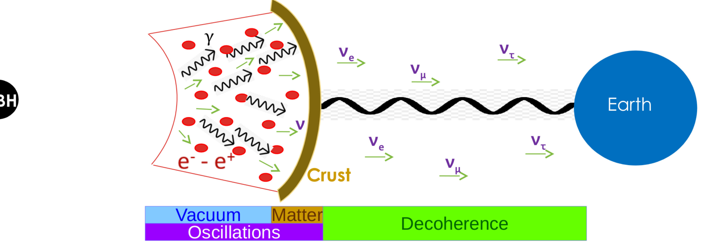 Figure 1
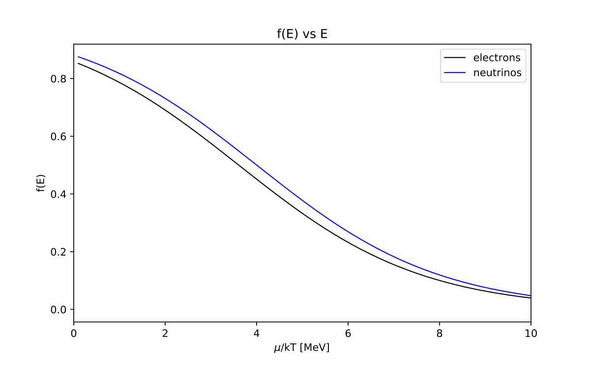 Figure 2
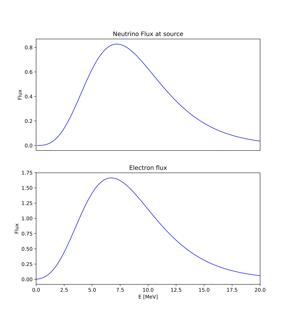 Figure 3
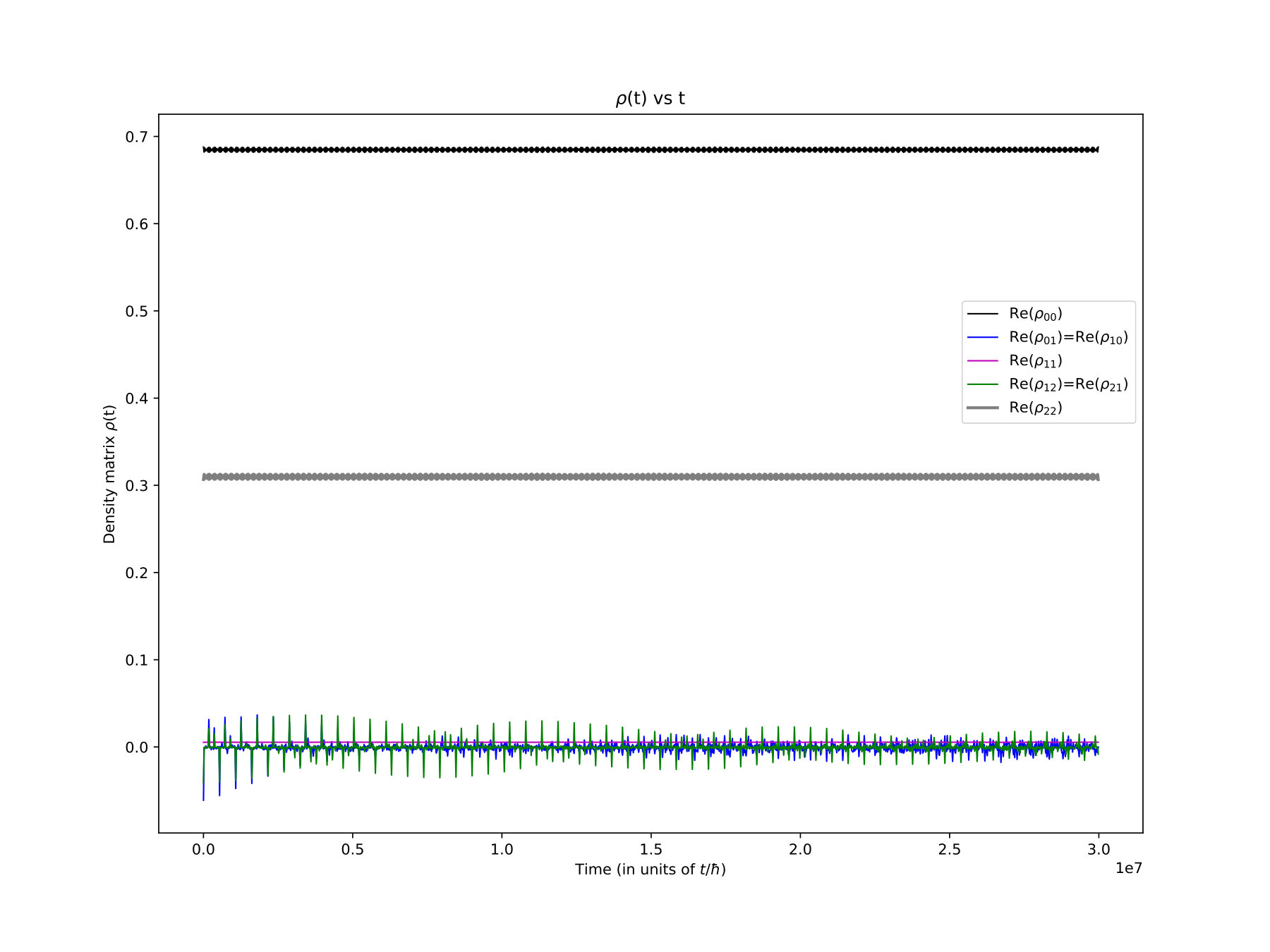 Figure 4
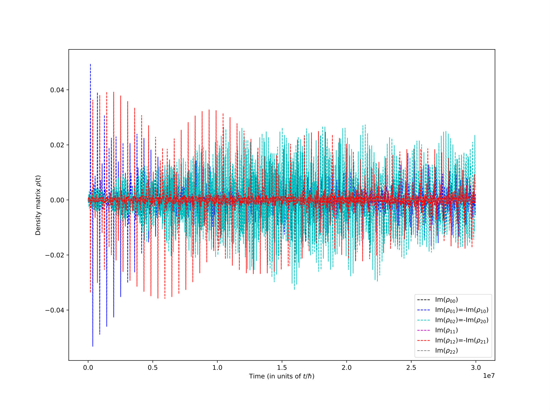 Figure 4
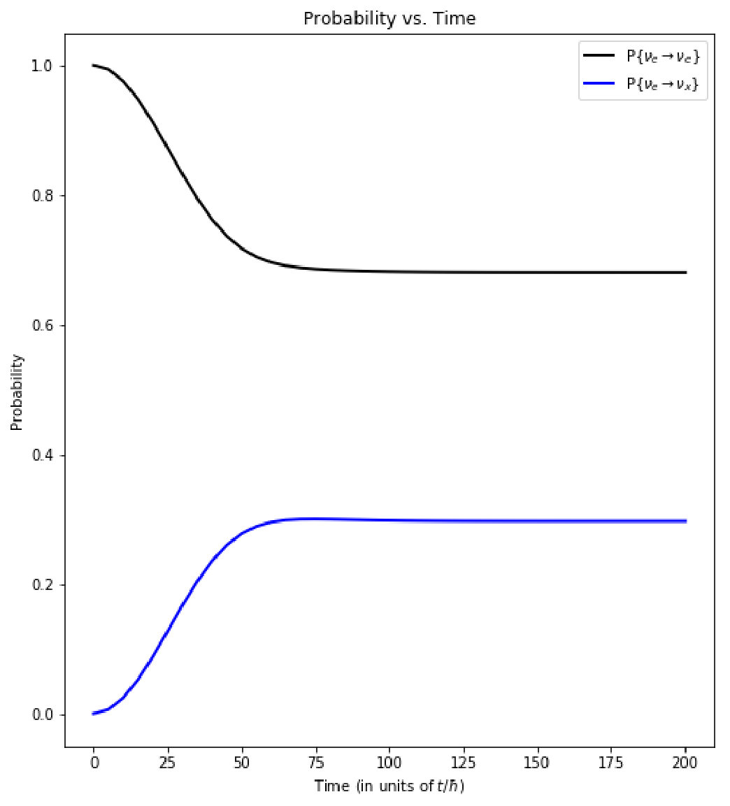 Figure 5
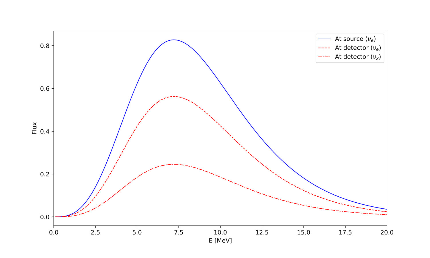 Figure 6
| Parameter | Symbol | Value |
| NS radius [km] | 10 | |
| NS mass [] | ||
| plasma density [part/cm3] | ||
| plasma temperature [MeV] | kT | 2.0 |
| BH radius [cm] | ||
| Crust internal radius [cm] | ||
| Crust external radius [cm] | ||
| Source-detector distance [cm] | ||
| Mass of the crust [] | 0.1 | |
| Density of the crust [g/cm3] | ||
| Proton density in the crust [part/cm3] | 0.25 | |
| Neutron density in the crust [part/cm3] | 0.25 | |
| density in the crust [part/cm3] | 0.50 |
| (NH) |
| (IH) |
| eV2 |
| eV2 |
Peer Reviews
No public reviews on file for this paper yet. If you reviewed it on a platform where reviews are public (OpenReview, ICLR, NeurIPS, ICML), you can paste yours below so the community can read it here.
Videos
No videos yet. Explain this paper in a talk, walkthrough, or lecture? Add one.
Neutrino oscillations and decoherence in short-GRB progenitors
A.V. Penacchioni
IFLP (CONICET), La Plata, Argentina
O. Civitarese
Department of Physics, University of La Plata (UNLP)
49 y 115 cc. 67, 1900 La Plata, Argentina
IFLP (CONICET), La Plata, Argentina
Abstract
Neutrinos are produced in cosmic accelerators, like active galactic nuclei (AGNs), blazars, supernova (SN) remnants and gamma-ray bursts (GRBs). On their way to the Earth they experience flavor-oscillations. The interactions of the neutrinos coming from the source with other particles, e.g. intergalactic primordial neutrinos or heavy-mass right-handed neutrinos, in their way to the detector may transform the original wave packet in pointer states. This phenomenon, known as decoherence, becomes important in the reconstruction of processes at the source. In this work we study neutrino emission in short GRBs by adopting the Fireshell Model. We consider -pair annihilation as the main channel for neutrino production. We compare the properties of the neutrino-flux with the characteristic photon-signal produced once the transparency condition is reached. We study the effects of flavor-oscillations and decoherence as neutrinos travel from the region near the black-hole (BH) event-horizon outwards. We consider the source to be in thermal equilibrium, and calculate energy distribution functions for electrons and neutrinos. To compute the effects of decoherence we use a Gaussian model. In this scenario the emitted electron-neutrinos transform into pointer states consisting of electron-neutrinos and as a combination of mu and tau neutrinos. We found that decoherence plays an important role in the evolution of the neutrino wave packet, leading to the detected pointer states on Earth.
neutrinos — gamma-ray bursts: general — astroparticle physics
\reportnum
Published in ApJ 2019, v872, id.76, 8pp.
\savesymboliint \savesymboliiint \savesymboliiiint \savesymbolidotsint \restoresymbolAMSiint \restoresymbolAMSiiint \restoresymbolAMSiiiint \restoresymbolAMSidotsint
1 Introduction
Short gamma-ray bursts (S-GRBs) are intense flashes of gamma-rays that last less than 2 seconds in the observer frame. It is widely accepted that S-GRBs originate from the merging of two compact objects, such as a neutron star (NS) and a BH, or two neutron stars (NS-NS). During the merging phase, angular momentum and energy losses are manifested as gravitational wave emission and electromagnetic radiation. In both cases the remnant is a BH of a few solar masses. There are different models which try to explain the observed emission of short GRBs; among others the Fireball Model (Piran 1999) and the Fireshell Model (Bianco et al. 2008a; Bianco & Ruffini 2008; Bianco et al. 2008b; Enderli et al. 2014).
The Fireball Model states that in the case of the NS-NS system an accretion-disk is formed around the newly born BH (Berger 2014). In the NS-BH case the same can occur if the NS is tidally disrupted outside the BH’s event horizon. The rapidly rotating BH bends the magnetic-field-lines forming a double-jet perpendicular to the accretion-disk plane. A fraction of the electromagnetic radiation escapes in the form of gamma-rays, while another fraction goes into neutrino-antineutrino emission (Narayan et al. 1992).
In the Fireshell Model scenario the NS-NS merging leads to a massive NS that exceeds its critical mass and gravitationally collapses to a BH with isotropic energy-emission of the order of erg. Gravitational waves are produced (Oliveira et al. 2014) together with GeV emission from the accretion onto the Kerr BH (Ruffini et al. 2018). It has been shown (Becerra et al. 2018) that the accretion onto the NS generates neutrino-antineutrino emission in the case of long GRBs, and this emission has been explained as due to -pair annihilation.
In this work we apply the Fireshell Model to explain neutrino emission in S-GRBs. We describe the conditions under which the neutrino emission takes place and we analyse the effects of flavor-oscillations and decoherence on neutrinos on their way from the source to the observer on Earth.
The work is organised as follows: in Section 2 we describe the model. In Section 3 we derive the expressions for the electron and neutrino number densities, following a statistical treatment. In Section 4 we compute the electron and neutrino fluxes at the source. In Section 5 we analyze the effects of neutrino-flavor oscillations in vacuum, from the moment in which neutrinos are produced up to the time they reach the external crust. In Section 6 we analyze the effects of neutrino-flavor oscillations in matter, as they propagate through the crust and interact with baryons. In Section 7 we introduce the mechanism of decoherence, since neutrinos which leave the crust and propagate through the Universe towards the observer, interact with background intergalactic particles. We calculate the detected flux on Earth and compare it with the flux at source. The results are presented and discussed in Section 7.3. Finally, in Section 8 we draw our conclusions.
2 The model
A typical scenario for S-GRBs within the Fireshell Model is depicted in Figure 1. Two NS of masses and , typically of the order of M⊙, start spiraling together until they merge giving birth to a BH due to gravitational collapse. Let us consider for simplicity . Only the core collapses, leaving a thin crust of a fraction of a solar mass. In the vacuum between the crust and the BH event-horizon a strong electric field is generated due to charge separation. When this field reaches the critical value, , vacuum polarization takes place generating an -plasma. Typical densities for the electron-positron plasma are of the order of particles/cm3. Some of these pairs annihilate giving neutrinos and antineutrinos which propagate outwards, first in vacuum then through the crust formed by , protons and neutrons, and finally through the intergalactic medium until they reach the observer on Earth (Halzen & Klein 2010; SNO Collaboration 2000). Another fraction of the -pairs produce thermal photons. Since at this stage the system is still opaque to radiation, the radiation pressure increases making the plasma expand until it reaches the crust. The whole system continues to expand until it reaches transparency. At this point the thermal photons escape. This is seen as a thermal spike in the spectrum called proper-GRB (P-GRB) (Ruffini et al. 2001). The remaining material continues to expand while interacting with the circumburst medium producing the prompt emission.
Table 1 shows the values of the parameters of our model.
3 Neutrino number density and energy
In order to calculate the number density and energy of the neutrinos created during the merging of the two NS, we follow a statistical treatment. We treat the neutrinos as a Fermi-Dirac gas in thermodynamical equilibrium at temperature MeV (Ruffini et al. 1999). The neutrino emission zone is the same as the one occupied by the -plasma, a shell that extends from the BH event-horizon ( cm) to the crust ( cm).
The Fermi-Dirac distribution function for is given by
[TABLE]
where is the Boltzmann constant and is the fermion energy. The parameter is known as the Fermi level. In the limit , becomes a step function : all the energy levels with are occupied, while all the others are empty.
3.1 Electrons
In the relativistic case the energy of the electrons is , the momentum in terms of the energy is given by , and . The number of particles in the system is given by the expression
[TABLE]
Here,
[TABLE]
is the volume element in phase space and is the spin degeneracy factor. Changing variables to yields the number density :
[TABLE]
By making the substitutions , and , Eq.3 becomes
[TABLE]
where
[TABLE]
for , etc.
A similar expression is obtained for the mean energy of the electrons as a function of temperature and density:
[TABLE]
3.2 Neutrinos
Neutrinos have negligible masses compared to their energy (), so . Following the same procedure as in Section 3.1 we find for the neutrino-number-density
[TABLE]
where
[TABLE]
for ,… and .
The neutrino mean energy is given by
[TABLE]
thus, the mean energy per neutrino is given by
[TABLE]
4 Electron and neutrino fluxes at source
With the parameters given in Table 1 and the formalism presented in Section 3 we have performed a numerical search to determine the electron and neutrino chemical potentials and , and with them the mean energies and spectral functions (Cox & Giuli 1968).
The numerical search gives from Eqs. 3 and 6 the best values of and for a given density. The results are , , corresponding to MeV and MeV. Figure 2 shows the occupation numbers of Eq. 1 for a plasma temperature of MeV (Ruffini et al. 1999).
We have calculated the electron and neutrino fluxes inside the -plasma. Each flux is given by the ratio
[TABLE]
Figure 3 shows the results of Eq. 9 for electron and neutrino fluxes in the region of the -plasma.
5 Neutrino oscillations in vacuum
As soon as they are created, neutrinos start to propagate outwards at nearly the speed of light from the region close to the event-horizon towards the crust. This region is opaque to radiation, but nothing prevents neutrinos from escaping. Because of the geometry of the source (see Figure 1) we shall consider propagation and oscillations in vacuum in the inner region between the BH and the crust.
Neutrinos oscillate because the flavor states in which they are created are a superposition of mass eigenstates. Since they have different masses they evolve with different phases.
The Hamiltonian in the mass basis is given by
[TABLE]
The mass hierarchies are denoted, as usual: (Normal Hierarchy), (Inverted Hierarchy), or (Degenerate Hierarchy). Adopting the normal hierarchy, and setting , yields eV and eV.
The neutrino mass Hamiltonian is transformed to the flavor basis by applying upon it the mixing matrix (Kersten & Smirnov 2016; Bilenky 2000)
[TABLE]
where () are the cosine (sine) of the mixing angles . Therefore,
[TABLE]
The parameters entering and are listed in Table 2. In the present analysis we have taken, for the Dirac CP-violating phase, the value . Furthermore, and in order to separate the electronic flavor from linear combinations of the and ones, we apply to the flavor Hamiltonian the decoupling matrix (Kersten & Smirnov 2016)
[TABLE]
The ‘decoupled’ flavor Hamiltonian reads
[TABLE]
and from the diagonalization of this Hamiltonian we obtain the eigenvalues and eigenvectors for electron neutrinos and non-electronic neutrinos .
6 Oscillations in matter
Following the model sketch in Figure 1, neutrinos oscillate in vacuum until they reach the internal radius of the crust. At this point, they interact with matter. We assume the crust is formed by electrons, protons and neutrons in the amounts given in Table 1. A matter Hamiltonian must be added to the flavor Hamiltonian in vacuum. For the matter Hamiltonian we consider a diagonal one
[TABLE]
where is the matter potential, MeV cm3 is the Fermi constant and , and are the electron, proton and neutron densities in the crust, respectively.
Because of the thickness of the crust ( cm) the interactions with matter are negligible despite the values of the baryon densities. Therefore, we shall not take these interaction into account in our analysis.
7 Decoherence
Once the neutrinos arrive at the external radius of the crust they continue their way to the detector on Earth. Since the distance that they have to travel is of the order of cm, corresponding to typical SGRB redshifts (Ruffini et al. 2016), decoherence effects (Schlosshauer 2007) may take place due to interactions of the source neutrinos with neutrinos in the cosmic background. Decoherence effects are relevant in the reconstruction of the sequence of events starting from the primordial production of neutrinos and ending at their detection. What we would like to evaluate quantitatively is the difference between the composition of neutrinos of the source, as dictated by the neutrino-oscillation mechanism, and their time evolution governed by decoherence. The decoherence mechanism we have in mind in not kinematic and, as we said before, it is due to interactions with other particles like neutrinos which fill the space between the source and the detector. In order to achieve this goal we shall proceed to:
Calculate the density matrix from the diagonalization of the flavor Hamiltonian (Eq.14). 2. 2.
Construct the time evolution matrix which determines the time dependence of the density matrix. 3. 3.
Calculate the probability of detecting neutrinos of a given flavor on Earth.
In what follows we present the corresponding theoretical details.
7.1 Flavor eigenstates at
The density matrix for electron-neutrinos leaving the crust is
[TABLE]
With the amplitudes of the electron-neutrino eigenvalue obtained by the diagonalization of , Eq.(16) is readily calculated.
The density matrix (Eq.16) is that of a pure state, that is , and its diagonalization yields the survival probabilities of the electron-, muon- and tau-neutrino channels, respectively.
7.2 Time dependence of the density matrix
To calculate the time dependence of the density matrix for neutrinos leaving the crust we add to the flavor Hamiltonian the interaction of the electron-neutrinos with the environment. For this, we follow the formalism presented in Bes & Civitarese (2017) and Schlosshauer (2007). Accordingly, we construct the matrix
[TABLE]
where is the coupling constant and is a constant field acting on the neutrinos. The diagonalization of leads to the eigenvalues and eigenvectors needed to construct the evolution matrix (Schlosshauer 2007), which is defined by the expression
[TABLE]
where is the matrix of eigenvectors of , , , the associated eigenvalues, being both and functions of the strength . In writing Eq.(18) we use . In this picture the density matrix of Eq.(16) evolves with time as
[TABLE]
If the strength is distributed like a Gaussian around with standard deviation , we integrate the matrix in B so that its elements are:
[TABLE]
A last diagonalization of for sufficiently large, of the order of , being the distance from the source to the detector and the speed of light, leads to the survival probabilities of neutrinos of a given flavor, in this case, of electron-neutrinos. These probabilities are needed in order to renormalise the neutrino flux at Earth, as explained below.
7.3 Results for and
For the normal hierarchy and masses , eV, eV and in Eq.(11), we get
[TABLE]
The diagonalization of gives
[TABLE]
To illustrate the effect of decoherence we calculate the time evolution given by Eq.20 with and .
For a sufficiently large number of oscillations in presence of the interactions due to the background and for the chosen parameterization, the density matrix is given by
[TABLE]
which is no longer the density matrix of a pure state, since .
Diagonalization of this matrix gives the survival probabilities:
[TABLE]
[TABLE]
Fig. 4 shows the elements of the density matrix as a function of time, as the system evolves to the pointer states.The fact that the matrix loses its pure-state nature due to decoherence is better illustrated by the results shown in Figure 5, where the final pointer states are identified by means of the probabilities and .
The neutrino flux, for neutrinos emitted at the source (see Fig.3), should then be renormalised to account for the evolution of from pure to pointer states. This is done by multiplying the curves of Figure 3 by the probabilities (24) and (25). The results are shown in Fig 6.
We shall calculate the characteristic wavelengths of flavor-oscillations to compare them with the size of the regions where the effects take place.
In the case of flavor-oscillations, the amplitude of the electron-flavor survival is given by
[TABLE]
and
[TABLE]
for the real and imaginary parts of the amplitude, respectively, with
[TABLE]
To make a rough estimation of the period of oscillations, we take the squared mass difference in the normal hierarchy and write for the period (Kersten & Smirnov 2016)
[TABLE]
The corresponding wavelength for flavor oscillations will then be
[TABLE]
For the neutrino mean energy obtained in our calculations, MeV, we have cm. This is much larger than the distance from the event horizon to the external part of the crust ( cm), therefore confirming the pure-state nature of the density matrix (Eq.16) for neutrinos leaving the source.
7.4 About the observability of the emitted neutrinos
The results which we have presented so far show that the survival probabilities for the emitted electron-neutrinos change considerably, as do the calculated fluxes at the source and at the detector. As mentioned before, Eq.9 gives the number of particles (electrons or neutrinos) with energies in the interval .
Köpke & IceCube Collaboration (2011) performed a simulation of a Supernova event at a distance of 10 kpc with total emitted energy of erg, starting from a M⊙ progenitor and considering inverse beta decay, neutron capture and positron annihilation as the main channels for neutrino interaction. They obtain a mean energy of the order of 15 MeV and a rate of counts/s. In our case, we consider a NS-NS merger leading to a M⊙ progenitor at a redshift , which corresponds to a distance of Mpc (or cm, as stated in Table 1), just like GRB 090510 (Rau et al. 2009). The only channel considered for neutrino production in our model is annihilation (we intend to extend the model by considering more production channels that contribute to the total neutrino flux in a future work). We obtain a neutrino mean energy per particle of MeV. The rate at the detector is thus of the order of events/s, which is far from being detected with the current Ice Cube sensitivity and effective area. However, this may be achieved by the future detector generations. What we would like to emphasize is that our calculations give us a mean neutrino energy which falls in the range of supernovae neutrinos (see Fig. 1 of Spiering (2012)).
8 Conclusions
In this work we have investigated the processes leading to the emission of neutrinos in short-GRB progenitors. Following the discussions advanced in the literature (Bianco & Ruffini 2008) we have modeled the system so that the -plasma is the main source of neutrinos. These neutrinos travel through the region between the BH event-horizon and the crust, their density matrix being that of pure states described by neutrino flavor-oscillations. Because of the astronomical scale of the distance between the source and the detector on Earth, decoherence effects due to interaction with the cosmic background may become important. We have calculated these effects by adopting a Gaussian model to incorporate the cosmic background.
The present calculations give a mean neutrino energy which falls in the range of SN neutrinos. The value of the predicted neutrino flux is still far away from observation but considering the continuous advances in detector technology it could be reachable by future generations of experiments.
Further work is in progress concerning the time delay between neutrino and photon emission in GRBs.
The authors would like to thank Dr. A. Marinelli for useful discussions. This work has been partially supported by the National Research Council of Argentina (CONICET) by the grant PIP 616, and by the Agencia Nacional de Promoción Científica y Tecnológica (ANPCYT) PICT 140492. A.V.P and O.C. are members of the Scientific Research career of the CONICET.
The reference list from the paper itself. Each links out to its DOI / PubMed record.
- 1Becerra et al. (2018) Becerra, L., Guzzo, M. M., Rossi-Torres, F., et al. 2018, Ap J, 852, 120, doi: 10.3847/1538-4357/aaa 296 · doi ↗
- 2Berger (2014) Berger, E. 2014, ARA&A, 52, 43, doi: 10.1146/annurev-astro-081913-035926 · doi ↗
- 3Bes & Civitarese (2017) Bes, D. R., & Civitarese, O. 2017, in American Institute of Physics Conference Series, Vol. 1894, American Institute of Physics Conference Series, 020006
- 4Bianco et al. (2008 a) Bianco, C. L., Bernardini, M. G., Caito, L., et al. 2008 a, in American Institute of Physics Conference Series, Vol. 966, Relativistic Astrophysics, ed. C. L. Bianco & S.-S. Xue, 12–15
- 5Bianco et al. (2008 b) Bianco, C. L., Bernardini, M. G., Caito, L., et al. 2008 b, in American Institute of Physics Conference Series, Vol. 1065, American Institute of Physics Conference Series, ed. Y.-F. Huang, Z.-G. Dai, & B. Zhang, 223–226
- 6Bianco & Ruffini (2008) Bianco, C. L., & Ruffini, R. 2008, in The Eleventh Marcel Grossmann Meeting On Recent Developments in Theoretical and Experimental General Relativity, Gravitation and Relativistic Field Theories, ed. H. Kleinert, R. T. Jantzen, & R. Ruffini, 1989–1991
- 7Bilenky (2000) Bilenky, S. M. 2000, Ar Xiv High Energy Physics - Phenomenology e-prints
- 8Cox & Giuli (1968) Cox, J. P., & Giuli, R. T. 1968, Principles of stellar structure