Coarse-graining Molecular Systems by Spectral Matching
Feliks N\"uske, Lorenzo Boninsegna, Cecilia Clementi

TL;DR
This paper introduces a spectral matching framework for coarse-graining molecular systems that preserves kinetic properties by aligning the low-lying spectrum of the system's generator, enabling more accurate long-time simulations.
Contribution
It presents a novel data-driven spectral matching approach that directly targets generator eigenvalues to improve coarse-grained models' kinetic accuracy.
Findings
Spectral matching effectively preserves slow dynamics in coarse-grained models.
The method can correct existing coarse-graining techniques like force matching.
Demonstrated improved retention of kinetic properties in molecular simulations.
Abstract
Coarse-graining has become an area of tremendous importance within many different research fields. For molecular simulation, coarse-graining bears the promise of finding simplified models such that long-time simulations of large-scale systems become computationally tractable. While significant progress has been made in tuning thermodynamic properties of reduced models, it remains a key challenge to ensure that relevant kinetic properties are retained by coarse-grained dynamical systems. In this study, we focus on data-driven methods to preserve the rare-event kinetics of the original system, and make use of their close connection to the low-lying spectrum of the system's generator. Building on work by Crommelin and Vanden-Eijnden, SIAM Multiscale Model. Simul. (2011), we present a general framework, called spectral matching, which directly targets the generator's leading eigenvalue…
Click any figure to enlarge with its caption.
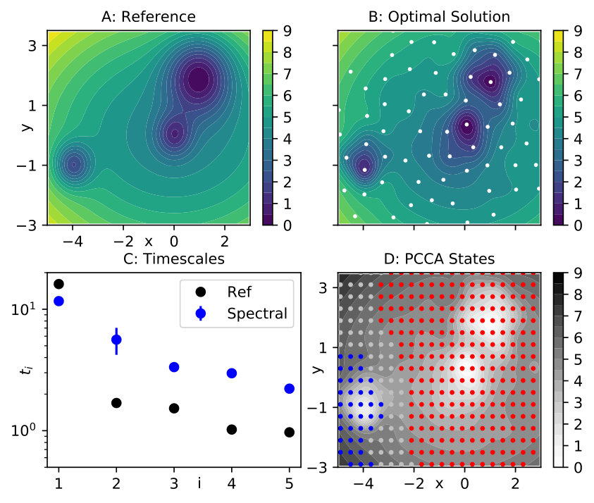 Figure 1
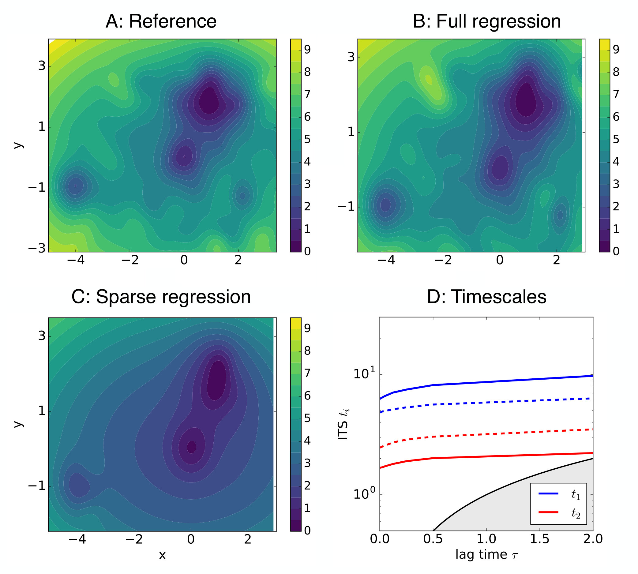 Figure 2
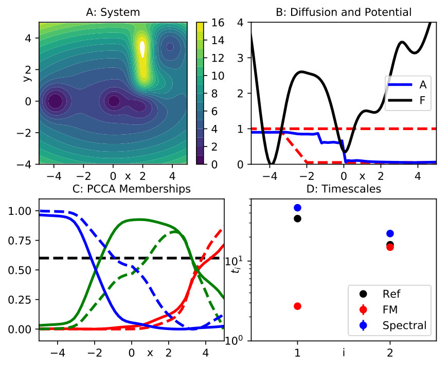 Figure 3
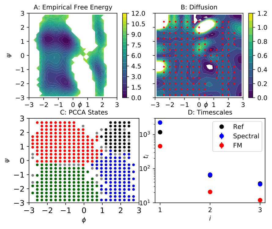 Figure 4
Peer Reviews
No public reviews on file for this paper yet. If you reviewed it on a platform where reviews are public (OpenReview, ICLR, NeurIPS, ICML), you can paste yours below so the community can read it here.
Videos
No videos yet. Explain this paper in a talk, walkthrough, or lecture? Add one.
Coarse-graining Molecular Systems by Spectral Matching
Feliks Nüske
Lorenzo Boninsegna
Cecilia Clementi
Center for Theoretical Biological Physics, and Department of Chemistry, Rice University
Abstract
Coarse-graining has become an area of tremendous importance within many different research fields. For molecular simulation, coarse-graining bears the promise of finding simplified models such that long-time simulations of large-scale systems become computationally tractable. While significant progress has been made in tuning thermodynamic properties of reduced models, it remains a key challenge to ensure that relevant kinetic properties are retained by coarse-grained dynamical systems. In this study, we focus on data-driven methods to preserve the rare-event kinetics of the original system, and make use of their close connection to the low-lying spectrum of the system’s generator. Building on work by Crommelin and Vanden-Eijnden, SIAM Multiscale Model. Simul. (2011), we present a general framework, called spectral matching, which directly targets the generator’s leading eigenvalue equations when learning parameters for coarse-grained models. We discuss different parametric models for effective dynamics and derive the resulting data-based regression problems. We show that spectral matching can be used to learn effective potentials which retain the slow dynamics, but also to correct the dynamics induced by existing techniques, such as force matching.
I Introduction
Coarse-graining or model reduction is the process of describing a high-dimensional and complex dynamical system by a smaller set of variables, and of providing a new set of governing equations for this reduced description. Coarse-graining has become a fundamental challenge in many different areas of science, such as finance, atmospheric science, or molecular biology. Two of the central reasons for the importance of coarse-graining are that, firstly, analysis or numerical simulation of high-dimensional systems is often challenging or simply infeasible, and secondly, not all detailed features of the full system are needed in order to answer questions of scientific interest. For molecular systems, important contributions to the field include coarse-graining in structural space, where the physical representation of a system is simplified. Several approaches have been proposed to design coarse-grained models for large molecular systems that either reproduce structural features of fine-grained (atomistic) models (bottom-up) Reith et al. (2003); Izvekov and Voth (2005); Noid et al. (2008); Shell (2008); Wang et al. (2009); Noid (2013) or reproduce experimentally measured properties for one or a range of systems (top-down) Lyubartsev and Laaksonen (1995); Nielsen et al. (2003); Marrink et al. (2004, 2007); Shinoda et al. (2007); Monticelli et al. (2008); Clementi (2008).
An alternative approach is coarse-graining in configurational space, where a transformation of variables is applied to arrive at a smaller set of descriptors. Notable examples along these lines are the Mori–Zwanzig formalism Mori (1965); Zwanzig (1973); Chorin et al. (2000, 2002); Hijón et al. (2010), conditional expectations Legoll and Lelièvre (2010); Zhang and Schütte (2017); Legoll et al. (2017), averaging and homogenization Pavliotis and Stuart (2008), Markov state models and related techniques Prinz et al. (2011); Noé and Clementi (2017), and diffusion maps Rohrdanz et al. (2011).
The starting point in the design of a coarse molecular model is the definition of the variables. The choice of the coarse coordinates is usually made by replacing a group of atoms by one effective particle, and is usually based on physical and chemical intuition. Because of the modularity of a protein backbone or a DNA molecule, popular models coarse-grain a macromolecule to a few interaction sites per residue or nucleotide, e.g., the and atoms for a protein Clementi et al. (2000); Matysiak and Clementi (2004); Davtyan et al. (2012). Alternative methods have been proposed to design coarse variables more systematically Ponzoni et al. (2015); Sinitskiy et al. (2012); Boninsegna et al. (2018a).
In this study, we are concerned with the inference of governing equations on the reduced set of variables, given that these descriptors have already been selected, and that simulation data of the full system is available. Several methods to learn the parameters of an effective dynamics from data of the full system have been proposed, most notably the force matching scheme Izvekov and Voth (2005); Noid et al. (2008) and the relative entropy method Shell (2008) (the two approaches are connected Rudzinski and Noid (2011)). Sparse learning of dynamical equations has been studied in Refs. Brunton et al. (2016); Boninsegna et al. (2018b). Most of the previous work was aimed at recovering correct thermodynamics of the reduced system, that is, the distribution sampled by the effective dynamics should equal the distribution of the projected original process. However, these methods do not determine the equations for a system’s dynamical evolution. That means that these methods may not be able to design coarse-grained models that can reproduce molecular dynamical mechanisms (e.g. large conformational changes or assembly mechanisms in protein systems). Here, we shift the focus to designing coarse-grained models that reproduce slow dynamical mechanisms of a fine-grained system, that is, timescales, metastable states and transitions in between them.
In principle, if the dynamical equations of the fine-grained model are known, the dynamics of the corresponding coarse-grained variables is given by the Mori-Zwanzig projection formalism Mori (1965); Zwanzig (1973); Chorin et al. (2000, 2002), which introduces a memory term. Even if the memory term can be simplified with the assumption of a separation of timescales, the estimation of the quantities involved in the Mori-Zwanzig approach is non trivial Hijón et al. (2010). However, here we are not interested in reproducing all timescales of the system, but just the slowest processes (e.g., conformational changes or assembly processes in protein systems). This fact allows us to bypass the Mori-Zwanzig approach to directly define an effective coarse-grained potential to satisfy this requirement. We build on a framework for parameter estimation of stochastic dynamics introduced in Refs. Crommelin and Vanden-Eijnden (2006, 2011). It exploits that slow dynamical processes are directly related to low-lying eigenvalues and associated eigenfunctions of the generator of the dynamics Davies (1982a, b). A broad range of methods is available to approximate these spectral components from simulation data of the full system Deuflhard et al. (2000); Prinz et al. (2011); Noé and Nüske (2013); Schütte and Sarich (2013); Nüske et al. (2014); Mardt et al. (2018). Hence, we argue that the same loss function can be used to learn coarse-grained dynamics if the focus is on reproducing the slow kinetics, and call the resulting framework the spectral matching estimator. We derive the optimization problems for two specific use cases of spectral matching: the first is to recover an effective potential within an overdamped dynamics, the second is to correct dynamics obtained from force matching by learning a position-dependent diffusion. Applications to several toy systems and molecular dynamics simulations of alanine dipeptide illustrate the capabilities of the method and highlight practical details, especially the importance of regularization.
II Theory
II.1 Full Space Dynamics
We consider a stochastic process attaining values in -dimensional space , where is typically large. In the case of a molecular system, represents the coordinates of the molecule at time . We assume the process solves a reversible stochastic differential equation (SDE):
[TABLE]
In this formulation, is a scalar potential, while is the diffusion, which is a field of symmetric positive definite matrices. The divergence is understood as applying the divergence operator to each row of . In the following, we will focus on instead of as all statistical properties of the process depend only on . Equation (1) is the general form of a reversible SDE, where reversibility holds with respect to the unique invariant density of , given by . A widely used example of Eq. (1) is the overdamped Langevin dynamics defined by a potential energy function and a constant diffusion , which is related to temperature and friction by :
[TABLE]
The generator associated to Eq. (1) is the second order differential operator:
[TABLE]
where the colon indicates the Frobenius inner product between matrices. The non-negative operator is self-adjoint on the space of functions square-integrable with respect to the weight function . We assume possesses a discrete set of increasing eigenvalues , with associated eigenfunctions . Each eigenvalue corresponds to the relaxation rate of a dynamical process in the system Pazy (1983), with characteristic (implied) timescale:
[TABLE]
We are particularly interested in metastable processes; in terms of the eigenspectrum of (3) that means that there is a cluster of eigenvalues close to , separated from all higher eigenvalues by a spectral gap Davies (1982b, a); Dellnitz and Junge (1999); Deuflhard et al. (2000). We can see from Eq. (4) that these low-lying eigenvalues correspond to slow relaxation processes. We thus assume that there is a separation of timescales between fast and slow processes in the molecular system of interest.
II.2 Reduced Dynamics
In this study, we consider coarse graining of the system (1) by projecting the state space into a lower-dimensional space . Following Refs Legoll and Lelièvre (2010); Zhang et al. (2016), this projection is realized by a coarse-graining map . Our objective is to replace (1) by another reversible SDE defined only on the lower-dimensional space :
[TABLE]
The effective potential and effective diffusion should meet the following two requirements:
Thermodynamic Consistency: The invariant density of (5) should equal the integral of the full state invariant measure over pre-images of :
[TABLE]
Here is the pre-image of under the coarse-graining map, and is the Jacobian of . Thus, the measure defined in (7) is the restriction of the full invariant measure to , multiplied by a correction factor accounting for the non-linear change of variables. If satisfies Eq. (6), the corresponding scalar potential is called the potential of mean force (pmf):
[TABLE] 2. 2.
Kinetic Consistency: The coarse-grained dynamics should retain the metastable part of the original dynamics (that is, the slow processes). This requirement can be expressed using the generator of (5):
[TABLE]
which is self-adjoint on the space of functions of square-integrable with respect to . The leading (non-zero) eigenvalues and eigenfunctions of should match the corresponding eigenvalues and eigenfunctions of the original system, that is, they should satisfy and , for (note that we always have ).
II.3 Force Matching
The thermodynamic consistency can be enforced by force Matching Izvekov and Voth (2005); Noid et al. (2008), a powerful technique to extract the potential of mean force from simulation data of the full system. It is based on the fact that the gradient of the pmf solves the following minimization problem Noid et al. (2008); Ciccotti et al. (2008):
[TABLE]
where the minimization is over all square-integrable vector fields of the reduced variables . In (11), is the scalar potential from Eq. (1), while is called local mean force. If sufficient simulation data of the full system is available, Eq. (10) can be replaced by a data-based regression:
[TABLE]
We note that force matching can also be applied if the original process is full Langevin dynamics in position and momentum space, and is a transformation of the position space only. One of the difficulties in the practical application of this method has been that, in general, a coarse-grained potential satisfying the thermodynamic consistency includes many-body terms that are not easily modeled in the energy functions. Recently, machine learning methods have been used to alleviate this problem Bejagam et al. (2018); Zhang et al. (2018); Wang et al. (2018); Chan et al. (2019).
II.4 Spectral Matching
In order to achieve kinetic consistency, we build on an idea presented in Refs. Crommelin and Vanden-Eijnden (2006, 2011) for parameter estimation in stochastic dynamics like Eq. (1). Given the leading spectral components of the full system, a parametric model for the generator, and a set of test functions , in Crommelin and Vanden-Eijnden (2006, 2011) it was suggested to minimize the discrepancy in the leading eigenvalue equations in a weak sense:
[TABLE]
Application of this idea to the coarse-grained case is based on two insights. First, if thermodynamic consistency holds, inner products in coarse-grained space can be estimated using data of the full system, as for any , we have Zhang et al. (2016):
[TABLE]
Second, we have recently shown Nüske et al. (2019) that it is indeed possible to find a kinetically consistent model if the full eigenfunctions can be well approximated by functions of the reduced variables, i.e. if
[TABLE]
holds for . Spectral approximation and validation techniques like TICA Pérez-Hernández et al. (2013), Markov state models Deuflhard et al. (2000); Prinz et al. (2011); Schütte and Sarich (2013); Bowman et al. (2014), the Variational Approach Noé and Nüske (2013); Nüske et al. (2014), or VAMPnets Mardt et al. (2018) (see below) can be used to obtain the approximations , and to verify that (16) holds.
Thus, given approximate spectral components , a set of test functions on the coarse-grained space, a parametric model for the coarse-grained generator, and data sampling the full space distribution , we can combine Eqs. (14 - 16) to define the spectral matching estimator:
[TABLE]
Alternatively, we can also have the model generator act on the test functions, which yields:
[TABLE]
Whether or not and are identical depends on whether the model generator is symmetric w.r.t. the inner product . In other words, the two are identical if the model dynamics are reversible with respect to the measure , or yet in other words, if the scalar potential of the model is induced by as .
III Methods
In this section, we discuss two specific use-cases for the spectral matching estimator, as well as details of the practical implementation of the method.
III.1 Estimation of a Scalar Potential
The first use-case arises from the assumption that the effective dynamics can be modeled using overdamped Langevin dynamics in a scalar potential , using a fixed constant diffusion . The resulting model generator is
[TABLE]
In particular, if the model is a linear expansion into given basis functions, i.e. , , spectral matching becomes a linear regression. In order to avoid the computation of second order derivatives for the eigenfunctions, we apply the model generator to the test functions (Eq. 20). We also include the zeroth spectral pair, as the corresponding matrix entries are non-zero, to obtain a regression matrix , and a data vector :
[TABLE]
We have found that regression (23) is often ill-conditioned and requires regularization. Below, we will use elastic net regularization Zou and Hastie (2005) with parameters , that is:
[TABLE]
III.2 Estimation of a Diffusion
Next, we consider the situation where an estimate of a thermodynamically consistent scalar potential is already available, for example by application of the force matching scheme. As a result, any parametric model for the diffusion results in a symmetric model generator, and the parameter dependent term in the loss function can be evaluated as:
[TABLE]
provided that is always symmetric. This formulation only requires first order derivatives, but we need to estimate those derivatives for the eigenfunctions. As a special case, we focus on a linear expansion into scalar multiples of the identity matrix, i.e. . Again, spectral matching leads to a linear regression:
[TABLE]
Positive definiteness of the diffusion is easily enforced in this setting, by requiring positivity of the scalar pre-factor at all data points. In fact, we will restrict the diffusion to satisfy pre-selected upper and lower bounds , which can in principle be position dependent. If data points are given, we add linear inequality constraints:
[TABLE]
for all . The full optimization problem (29) then turns into a quadratic programming problem.
III.3 Variational Approach
The spectral matching approach discussed above requires an estimate of the eigenfunctions and eigenvalues of the original system. In order to compute approximations of a system’s dominant eigenfunctions and corresponding eigenvalues , we make use of the Variational Approach to Conformational Dynamics (VAC) Noé and Nüske (2013); Nüske et al. (2014), which is a data-driven method to represent the dominant eigenfunctions from a given library of basis functions. Below, the library will either consist of Gaussian functions or of piecewise constant functions, in which case the method is called a Markov state model Deuflhard et al. (2000); Prinz et al. (2011); Schütte and Sarich (2013); Bowman et al. (2014). Both techniques are employed to obtain the approximations required as inputs to the spectral matching, and also to analyze simulation data of the effective dynamics obtained from spectral matching. In order to extract a decomposition of state space into metastable sets, based on the dominant eigenfunctions, we use the PCCA algorithm Deuflhard and Weber (2005); Röblitz and Weber (2013). The software implementation we use is the pyEmma package Scherer et al. (2015).
IV Results
IV.1 Three Well Potential
We first illustrate the idea of spectral matching to model the overdamped Langevin dynamics (Eq. 22) in a two-dimensional toy potential. The energy function is given as a sum of three Gaussians and a harmonic confinement, that is:
[TABLE]
The actual values of the parameters are , , , , and ; a contour of the energy is shown in Fig. 1 A. The diffusion constant is . We generate a long equilibrium simulation of these dynamics, at integration time step , spanning time steps.
We use a Markov state model based on a grid discretization of the two-dimensional state space to compute the slow eigenfunctions and eigenvalues of the system. The slowest process corresponds to the transition out of the shallow minimum on the left into the center, it occurs at a timescale . The rest of the spectrum is separated from this process and there is no other distinct slow motion to be identified, see the black dots in Fig. 1 D. We thus set (that is, we use only the first non-trivial eigenfunction) and extract the approximate eigenfunction from the MSM.
We attempt to reproduce the energy in two-dimensional space from data, while not applying any model reduction. We employ spectral matching and a linear model in combination with the elastic net as in Eq. (26). A regular space clustering of the data at minimum distance 0.8 helps us define a set of 82 spherical Gaussian functions centered at the cluster centers, as shown in Fig. 1 B. These centers serve to define the test set, while the basis set consists of the same Gaussians plus the quadratic functions (). We use uniform widths and for all Gaussians in the basis set and the test set, respectively. We fix , while and both elastic net parameters are treated as hyper-parameters. They are determined by 3-fold cross-validation (CV) for all triples of the form . The optimal parameter set is , the corresponding solution is displayed in Fig. 1 B and agrees well with the original energy landscape in panel A.
Using the same simulation parameters as for the original system, we generate a realization of the dynamics defined by the optimized potential. An MSM analysis confirms that the slowest timescale is indeed well reproduced by those dynamics, see Fig. 1 C. As only the first non-trivial eigenfunction was used in the spectral matching, we do not expect to reproduce additional timescales besides the slowest one. Moreover, application of 2-state PCCA to this Markov model also shows that the decomposition of state space into metastable sets is the same as for the original potential, as displayed in panel D of Fig 1.
IV.2 Three Well Potential with Roughness
Here, the performance of the spectral matching is tested on a perturbed version of the three well potential investigated in section IV.1, to which small amplitude Gaussians were added; i.e.,
[TABLE]
with , and indicating the center of the -th perturbing Gaussian; a contour plot of such a potential is shown in Fig. 2 A. The diffusion constant is . We generate a long equilibrium simulation of these dynamics, at integration time step , spanning time steps.
The dominant timescales and eigenfunctions were numerically approximated using the VAC and a basis of 196 Gaussian features.
Spectral matching was applied to the data set, as exactly the same functions entering the linear combination Eq. (34) were employed both as basis and test functions in the procedure. Eventually, the full set of coefficients is approximated and compared with the exact result. Regression was solved using standard implementations, with and without elastic net regularization. The first two non-trivial eigenpairs were used in the spectral matching (that is, in Eq. 20).
The non-regularized solution is shown in Fig. 2 B and almost perfectly reproduces the exact potential, panel A. The regularized solution is shown in panel C, and the optimal regularization hyper-parameters were identified by running 3-fold CV on all tuples of the form . The solution is very sparse, only coefficients (out of the full set of ) have non-zero values. The position of the three main energy wells is correctly identified, which correlate with the system’s slowest dynamics, while most of roughness of the potential is washed out. Regularization appears to be a physically meaningful procedure, since it systematically filters perturbations, i.e., rugged local minima, out.
However, the wells are shallower than expected, compare with Fig. 2 A. In order to investigate if this observation has any effect, a long equilibrium trajectory was generated by integrating overdamped Langevin dynamics, using the optimal solution as potential energy (), and the associated timescales were estimated using VAC in the same setup as before. Results are shown in Fig. 2 D, where the resulting two slowest timescales (red) are compared to the reference ones (blue): the processes occur on very similar timescales.
IV.3 Recovery of Slow Kinetics by Non-Constant Diffusion
Next, we demonstrate that spectral matching can be used to recover the slow kinetics of a projected system with the aid of a non-constant diffusion. We consider a modified three-well system (Fig. 3 A), where the locations of the minima have been changed, and additional peaks have been added to the landscape. The slowest process is now the transition out of the shallow minimum on the right. An equilibrium simulation of 10 million frames at integration time step serves as the reference data set.
We estimate the reduced dynamics along the first coordinate . We apply force matching using a basis of 71 Gaussian functions centered at grid spacing 0.2 between and . A uniform width is selected by means of CV from the set . The estimated potential of mean force for the optimal value is represented by the black line in Fig 3 B.
We generate simulation data of overdamped Langevin dynamics in the potential of mean force, at diffusion (using the same integration time step and number of frames as for the full system). An MSM analysis of these data shows that the slowest timescale is decreased by a factor ten, while the next timescale is almost unaffected by the projection, see Fig. 3 D. Thus, the order of the two timescales is reversed, and the slow kinetics cannot be recovered by simply re-scaling the effective diffusion constant .
Spectral matching in the form (29) is applied to estimate a position-dependent diffusion. Approximate rates are extracted from a Markov state model of the full process. As the approximate eigenfunctions need to be functions of in Eq. (29), we build another MSM along alone and extract those approximate eigenfunctions. Even though this MSM does not yield accurate estimates of both timescales, the corresponding eigenfunctions still capture the structure of both slow transitions correctly, as we can see by looking at the corresponding PCCA memberships (solid lines in Fig. 3 C). The test set is chosen as the same basis set used for force matching. As a basis set, we choose a set of piecewise constant functions, where the corresponding discrete sets are obtained by partitioning the interval into equal-sized parts. The optimal choice for is again obtained by 3-fold cross validation on the hyper-parameter set .
It is important to solve Eq. (29) subject to position dependent lower bounds . Based on our analysis of the full data and the force matching simulation, we require , that is, close to one, in the left metastable set, while we set everywhere else. We also use as a global upper bound. The resulting optimal diffusion is indicated by the blue line in Fig. 3 B. This solution tends to slow down the transition out of the rightmost metastable state, while leaving the timescale of transition out of the center state unchanged. After running the effective dynamics (5) for 10 million steps at , and analyzing these data by an MSM, we find that both timescales are indeed approximately restored, see Fig. 3 D. These effective dynamics are more diffusive than the original system, as is reflected in the corresponding PCCA memberships being less crisp (dashed lines in Fig. 3 C). The change in the dynamics to restore the correct timescales perturbs the position of the metastable sets. However, the three metastable sets of the original dynamics are approximately retained.
IV.4 Alanine Dipeptide
Finally, we study model reduction of a small molecular system, alanine dipeptide, which has served as a test case for numerous studies in recent years. The data set at our disposal is the same that was used in Ref. Wang et al. (2018), please see Ref. Nüske et al. (2017) for the detailed simulation setup. It comprises one million frames of Langevin dynamics in explicit water saved every one picosecond.
It is well known that the system’s metastable processes are effectively functions of its two backbone dihedral angles . Therefore, we study reduction of this system into the two-dimensional space of those dihedral angles. Figure 4 A shows the empirical free energy in this space. It presents a more challenging example than the toy systems, as the coarse graining map is non-linear, and the metastability is much more pronounced in the sense that there are large unsampled areas and we only have very few samples in the transition regions. To simplify matters, we shift both dihedrals in order to eliminate almost all periodicity from this representation, and use non-periodic basis functions in what follows.
To obtain the approximate eigenfunctions and eigenvalues , we apply the VAC with 225 spherical Gaussian functions centered on a regular grid between -2.8 and +2.8 at a distance of 0.4 in each direction. Their widths are uniformly set to 0.3. We retain the first three non-trivial slow eigenfunctions, and the corresponding implied timescales are , , and . The corresponding transitions in dihedral space occur, respectively, between the left and right half of the plane, between the two minima on the left, and between the two shallow minima on the right.
We use spherical Gaussian functions to represent the force matching potential and to serve as basis and test functions in the spectral matching. The centers are placed on a regular grid with grid spacing 0.4 in all directions, but we remove centers in unpopulated areas of the state space. As a result, a set of 152 centers for Gaussian basis functions is obtained. For force matching, we employ 3-fold cross validation to determine a uniform width out of the parameter set , to yield an optimal value . To ensure that the resulting potential is confining, we evaluate the solution on a fine grid, and replace its values at unsampled grid points by a function that grows quadratically with the distance to the sampled area. A two-dimensional spline is fitted to this data to yield the final approximation.
To evaluate the kinetic properties of the force matching model, we generate a set of 100 overdamped Langevin simulations of length at constant diffusion . By comparing the three slowest timescales of these dynamics to the reference values (red and black dots in Fig. 4 D), we find that the force matching dynamics are uniformly accelerating the kinetics by about a factor three.
For spectral matching, we use the optimal Gaussian functions from force matching to serve as test functions, and also use the same centers to define the basis set. These centers are indicated by red markers in Fig. 4 B. We globally set , and apply 3-fold CV to determine the widths of the basis set, where . The solution of Eq. (29) for the optimal parameter value is shown in Fig. 4 B. The resulting diffusion is mostly constant at a value close to 0.3 throughout most of the domain, except for some peaks in boundary or unsampled regions. By generating another set of 100 simulations of simulation time each, we confirm that all three timescales are corrected by applying the optimized diffusion on top of the scalar potential, see Fig. 4 D, blue dots. By applying four-state PCCA to the effective simulations, we also verify the corresponding metastable sets to coincide with those of the original dynamics, see Fig. 4 C. Thus, the spectral matching enables us to find a (mostly constant) diffusion term in order to correct the coarse-grained system’s kinetic properties.
As a further consistency check, we also apply spectral matching with just a single basis function, which is the constant, while leaving all other settings unchanged. The resulting expansion coefficient, which is nothing more than an effective diffusion constant, also equals 0.3.
V Conclusions
We have introduced spectral matching as a method to define effective coarse-grained models reproducing the dynamics of a fine-grained system. Spectral matching can be used as stand alone or in combination with the existing force-matching method. While force matching enforces thermodynamic consistency, spectral matching enforces kinetic consistency. The goal of spectral matching is to retain slow processes of the original dynamics, while faster motions are considered less relevant and may be lost in the process. For two specific settings, we have presented the resulting data-based regression problems that follow from spectral matching. The first setting is the estimation of an effective potential for an overdamped dynamics, the second is concerned with learning an effective diffusion to correct the kinetics induced by force matching. We have demonstrated by several examples that spectral matching can be used to learn governing equations which retain the slow part of the dynamics. We found that suitable regularization is vital to the success of the method.
Several questions are left open for future work. While we were able to use relatively simple basis sets here, the application of the method to large molecular systems will require the use of more powerful model classes. Using deep learning, or other state of the art machine learning techniques, in conjunction with spectral matching is the topic of ongoing research. A better theoretical understanding of the method is also required. For instance, the limiting behavior of spectral matching if the test and basis sets become exhaustive needs to be addressed, especially in the case where a potential different from the pmf is estimated by spectral matching. Moreover, we found in many cases that multiple different solutions with almost equivalent kinetic properties can be found by spectral matching. A systematic treatment of this phenomenon will also follow in future work.
The reference list from the paper itself. Each links out to its DOI / PubMed record.
- 1Reith et al. (2003) D. Reith, M. Pütz, and F. Müller-Plathe, J. Comput. Chem. 24 , 1624 (2003).
- 2Izvekov and Voth (2005) S. Izvekov and G. A. Voth, J. Phys. Chem. B 109 , 2469 (2005).
- 3Noid et al. (2008) W. Noid, J.-W. Chu, G. S. Ayton, V. Krishna, S. Izvekov, G. A. Voth, A. Das, and H. C. Andersen, J.Chem. Phys. 128 , 244114 (2008).
- 4Shell (2008) M. S. Shell, J. Phys. Chem. 129 , 144108 (2008).
- 5Wang et al. (2009) Y. Wang, W. G. Noid, P. Liu, and G. A. Voth, Phys. Chem. Chem. Phys. 11 , 2002 (2009).
- 6Noid (2013) W. G. Noid, J. Phys. Chem. 139 , 090901 (2013).
- 7Lyubartsev and Laaksonen (1995) A. P. Lyubartsev and A. Laaksonen, Phys. Rev. E 52 , 3730 (1995).
- 8Nielsen et al. (2003) S. O. Nielsen, C. F. Lopez, G. Srinivas, and M. L. Klein, J. Chem. Phys. 119 , 7043 (2003).