Deep Iterative Surface Normal Estimation
Jan Eric Lenssen, Christian Osendorfer, Jonathan Masci

TL;DR
This paper introduces a novel end-to-end differentiable deep learning method for estimating surface normals from unstructured point clouds, combining interpretability, robustness, and efficiency.
Contribution
It proposes a graph neural network-based iterative algorithm that adaptively weights local plane fitting, outperforming previous methods without needing handcrafted features.
Findings
State-of-the-art accuracy in normal estimation
Robust to noise, outliers, and density variation
More than 100x faster and more parameter-efficient
Abstract
This paper presents an end-to-end differentiable algorithm for robust and detail-preserving surface normal estimation on unstructured point-clouds. We utilize graph neural networks to iteratively parameterize an adaptive anisotropic kernel that produces point weights for weighted least-squares plane fitting in local neighborhoods. The approach retains the interpretability and efficiency of traditional sequential plane fitting while benefiting from adaptation to data set statistics through deep learning. This results in a state-of-the-art surface normal estimator that is robust to noise, outliers and point density variation, preserves sharp features through anisotropic kernels and equivariance through a local quaternion-based spatial transformer. Contrary to previous deep learning methods, the proposed approach does not require any hand-crafted features or preprocessing. It improves on…
Click any figure to enlarge with its caption.
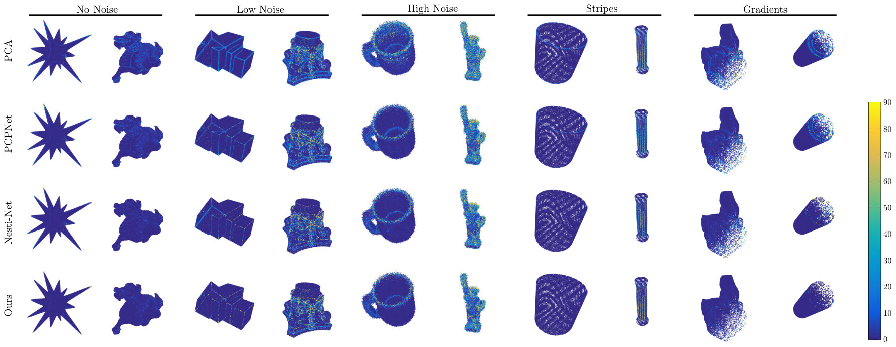 Figure 1
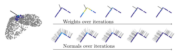 Figure 2
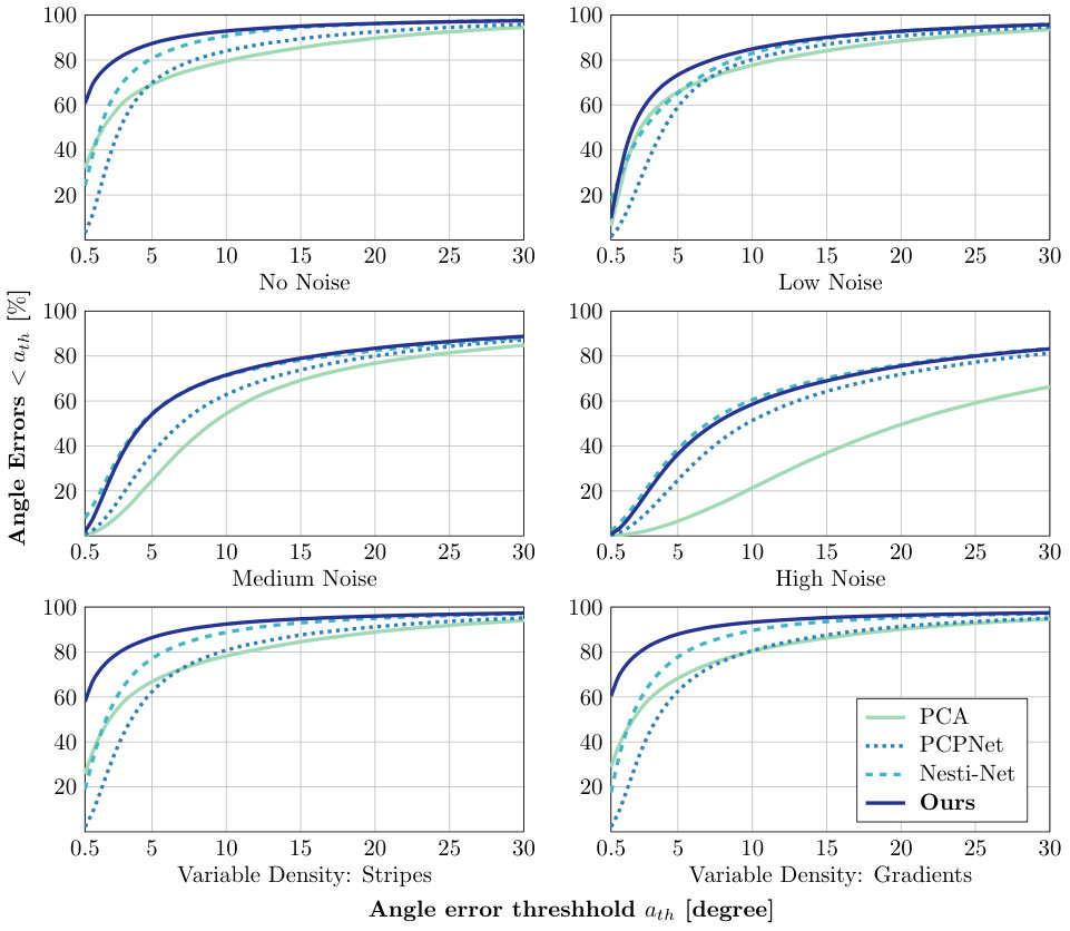 Figure 3
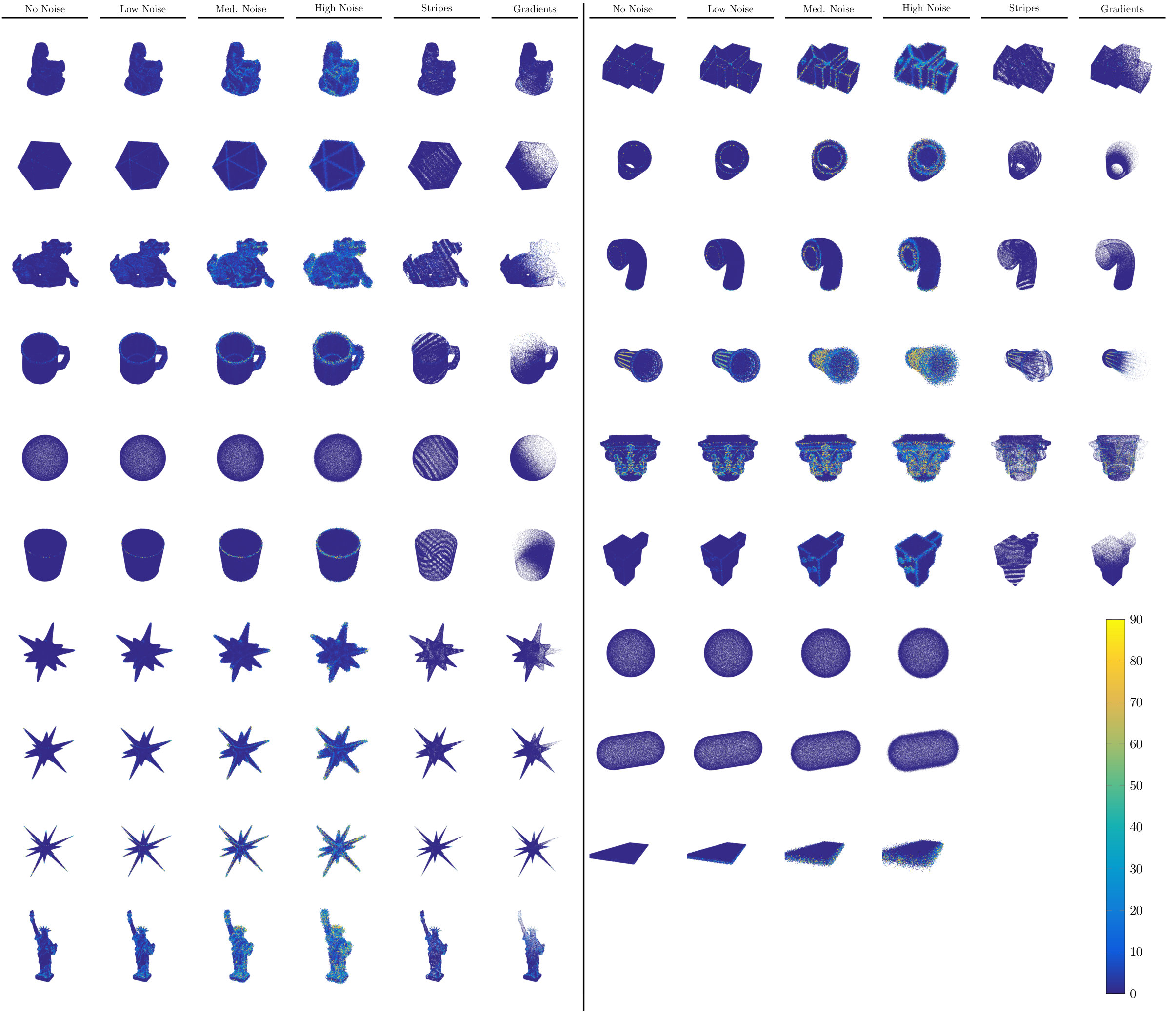 Figure 4
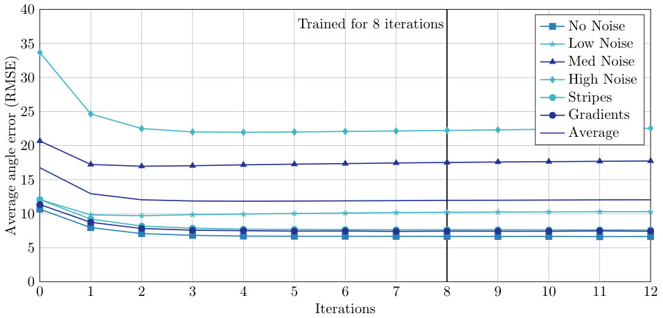 Figure 5
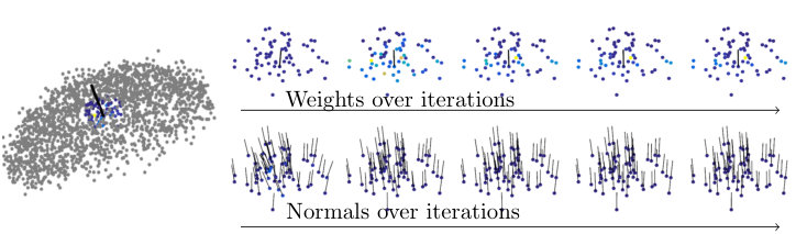 Figure 6
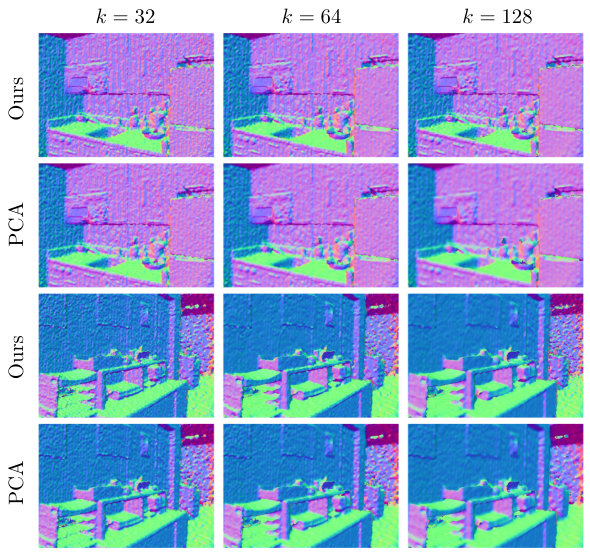 Figure 7
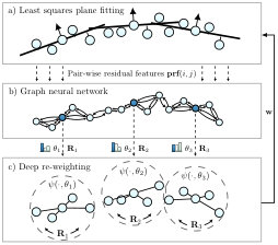 Figure 8
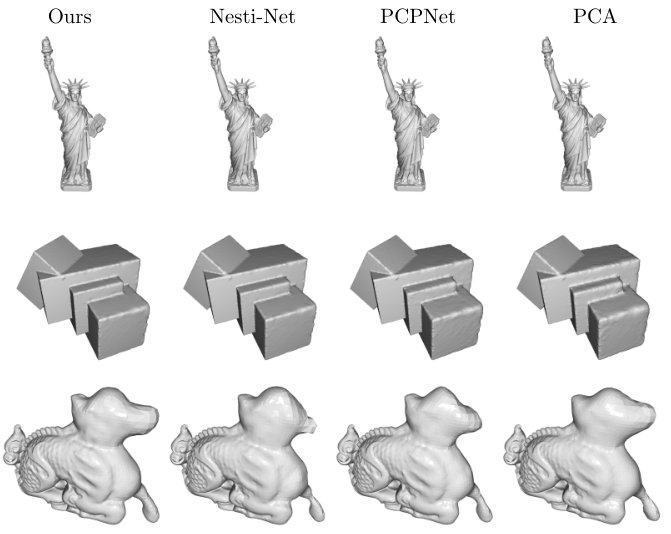 Figure 9
| Ours (, ) | Nesti-Net [5] | PCPNet [19] | HoughCNN [7] | PCA | Jet [9] | |
|---|---|---|---|---|---|---|
| No noise | 6.72 | 6.99 | 9.68 | 10.23 | 12.29 | 12.23 |
| Noise () | 9.95 | 10.11 | 11.46 | 11.62 | 12.87 | 12.84 |
| Noise () | 17.18 | 17.63 | 18.26 | 22.66 | 18.38 | 18.33 |
| Noise () | 21.96 | 22.28 | 22.8 | 33.39 | 27.5 | 27.68 |
| Varying Density (Stripes) | 7.73 | 8.47 | 11.74 | 12.47 | 13.66 | 13.39 |
| Varying Density (Gradients) | 7.51 | 9.00 | 13.42 | 11.02 | 12.81 | 13.13 |
| Average | 11.84 | 12.41 | 14.56 | 16.9 | 16.25 | 16.29 |
| Ours | PCA | |||||||||
|---|---|---|---|---|---|---|---|---|---|---|
| Neighborhood size | 32 | 48 | 64 | 96 | 128 | 32 | 48 | 64 | 96 | 128 |
| No noise | 6.09 | 6.63 | 6.72 | 6.82 | 7.35 | 9.10 | 9.94 | 10.68 | 11.93 | 12.54 |
| Noise () | 10.22 | 9.63 | 9.95 | 10.45 | 9.64 | 11.22 | 11.56 | 12.08 | 12.71 | 12.97 |
| Noise () | 18.17 | 17.36 | 17.18 | 17.03 | 16.90 | 28.41 | 23.00 | 20.68 | 18.81 | 18.12 |
| Noise () | 25.17 | 22.40 | 21.96 | 21.80 | 22.13 | 45.35 | 38.48 | 33.67 | 28.81 | 26.67 |
| Varying Density (Stripes) | 7.22 | 7.63 | 7.73 | 7.87 | 8.67 | 10.48 | 11.40 | 12.07 | 13.18 | 14.07 |
| Varying Density (Gradients) | 6.84 | 7.19 | 7.51 | 7.69 | 8.49 | 9.96 | 10.74 | 11.35 | 12.36 | 13.21 |
| Average | 12.28 | 11.81 | 11.84 | 11.94 | 12.20 | 19.09 | 17.52 | 16.75 | 16.30 | 16.26 |
| Network | Architecture | ||
|---|---|---|---|
| , | , | ||
| , | , | ||
| , | , | ||
| , | , | ||
| , | , | ||
| , | , | ||
| , | , | ||
| Trained on | Trained on | Trained on | |||||||||||||
|---|---|---|---|---|---|---|---|---|---|---|---|---|---|---|---|
| 32 | 48 | 64 | 96 | 128 | 32 | 48 | 64 | 96 | 128 | 32 | 48 | 64 | 96 | 128 | |
| No noise | 6.09 | 6.96 | 7.43 | 8.25 | 8.77 | 6.13 | 6.47 | 6.72 | 7.10 | 7.27 | 6.66 | 7.01 | 7.24 | 7.29 | 7.35 |
| Noise () | 10.22 | 10.01 | 10.09 | 10.37 | 10.62 | 10.19 | 9.93 | 9.95 | 10.18 | 10.35 | 9.89 | 9.57 | 9.50 | 9.50 | 9.64 |
| Noise () | 18.17 | 17.44 | 17.22 | 17.08 | 17.05 | 18.28 | 17.43 | 17.18 | 17.01 | 16.94 | 20.98 | 18.40 | 17.63 | 17.07 | 16.90 |
| Noise () | 25.17 | 22.97 | 22.33 | 21.91 | 21.80 | 25.20 | 22.53 | 21.96 | 21.69 | 21.67 | 30.99 | 24.94 | 23.20 | 22.34 | 22.13 |
| Density (Stripes) | 7.22 | 7.92 | 8.51 | 9.43 | 9.90 | 7.21 | 7.55 | 7.73 | 8.16 | 8.34 | 7.80 | 8.14 | 8.37 | 8.61 | 8.67 |
| Density (Gradients) | 6.84 | 7.46 | 8.06 | 8.80 | 9.21 | 6.89 | 7.17 | 7.51 | 8.04 | 8.03 | 7.48 | 7.75 | 8.11 | 8.39 | 8.49 |
| Average | 12.28 | 12.12 | 12.27 | 12.64 | 12.89 | 12.31 | 11.85 | 11.84 | 12.00 | 12.10 | 13.97 | 12.63 | 12.34 | 12.20 | 12.20 |
| Trained on | ||||||
|---|---|---|---|---|---|---|
| 2 | 4 | 8 | 16 | 24 | 32 | |
| No noise | 17.26 | 7.23 | 5.63 | 5.36 | 5.77 | 6.09 |
| Noise () | 54.02 | 49.66 | 33.65 | 13.80 | 10.74 | 10.22 |
| Noise () | 61.08 | 60.91 | 55.32 | 28.17 | 19.78 | 18.17 |
| Noise () | 61.29 | 61.26 | 58.89 | 41.37 | 28.99 | 25.17 |
| Density (Stripes) | 19.50 | 8.14 | 6.53 | 6.36 | 6.71 | 7.22 |
| Density (Gradients) | 22.89 | 8.44 | 6.51 | 6.23 | 6.57 | 6.84 |
| Average | 39.34 | 32.59 | 27.75 | 16.88 | 13.09 | 12.28 |
Peer Reviews
No public reviews on file for this paper yet. If you reviewed it on a platform where reviews are public (OpenReview, ICLR, NeurIPS, ICML), you can paste yours below so the community can read it here.
Code & Models
Videos
Deep Iterative Surface Normal Estimation· youtube
Taxonomy
Topics3D Shape Modeling and Analysis · Computer Graphics and Visualization Techniques · Advanced Numerical Analysis Techniques
MethodsInterpretability
Deep Iterative Surface Normal Estimation
Jan Eric Lenssen1,2,
[email protected] Work performed during an internship at NNAISENSE.
Christian Osendorfer1
1 NNAISENSE
2 TU Dortmund University
Jonathan Masci1
Abstract
This paper presents an end-to-end differentiable algorithm for robust and detail-preserving surface normal estimation on unstructured point-clouds. We utilize graph neural networks to iteratively parameterize an adaptive anisotropic kernel that produces point weights for weighted least-squares plane fitting in local neighborhoods. The approach retains the interpretability and efficiency of traditional sequential plane fitting while benefiting from adaptation to data set statistics through deep learning. This results in a state-of-the-art surface normal estimator that is robust to noise, outliers and point density variation, preserves sharp features through anisotropic kernels and equivariance through a local quaternion-based spatial transformer. Contrary to previous deep learning methods, the proposed approach does not require any hand-crafted features or preprocessing. It improves on the state-of-the-art results while being more than two orders of magnitude faster and more parameter efficient.
1 Introduction
Normal vectors are local surface descriptors that are used as an input for several computer vision tasks ranging from surface reconstruction [27] to registration [39] and segmentation [17]. For this reason, the task of surface normal estimation has been an important and well studied research topic for a long time, with several methods dating back up to 30 years [23]. Progress in the field, however, has been plateauing only until recently when a number of works has shown that improvements can be achieved with the use of data-driven deep learning techniques [5, 7, 19], as also shown in related fields like point cloud denoising [42] or finding correspondences on meshes and point clouds [10, 14, 32, 35]. Deep learning methods are known to often achieve better results compared to data-independent methods. However, they have downsides in terms of robustness to small input changes, adversarial attacks, interpretability, and sometimes also computational efficiency. Also, they do not make use of often well-known instrinsic problem structure, which leads to the necessity of having a large amount of training data and model parameters to learn that structure on their own.
It is well-known that surface normal estimation can be formulated as a least-squares optimization problem. A way to utilize this problem-specific knowledge with deep learning is to take an iteratively reweighting least squares (IRLS) scheme [22] for robust model fitting and modify it using deep data-dependent weighting, as it has been done recently (with or without iterations) for other tasks [25, 43, 44, 46]. It is a promising candidate to combine robustness, interpretability and efficiency with the data prior of deep neural networks (DNNs). From a deep learning perspective, the approach imposes a strong bias on the architecture, heavily constraining the space of solutions to those which are better suited for the given problem.
Contribution
In this work, we present such a trainable re-weighting procedure for input graphs with a large number of weighted least square problems and use it to design a fast and accurate algorithm for surface normal estimation on unstructured point clouds (c.f. Figure 1). The method consists of a light-weight graph neural network (GNN), which parameterizes a local quaternion transformer and a deep kernel function to iteratively re-weight graph edges in a large-scale point neighborhood graph. We show that the resulting algorithm
- •
reaches state-of-the-art performance in surface normal estimation on unstructured point clouds,
- •
is more than two orders of magnitude faster and more parameter efficient than related deep learning approaches, and
- •
is robust to noise and point density variation, while being equivariant and able to preserve sharp features.
2 Related work
Traditional methods for surface normal estimation make use of plane fitting approaches like unweighted principal component analysis (PCA) [23] and singular value decomposition (SVD) (c.f. [28] for an overview). The performance of these approaches usually hinges upon the often cumbersome selection of data-specific hyper-parameters, such as point neighborhood sizes, and it is sensitive to noise, outliers and density variations. Because of this, several heuristics have been proposed to ease such selection, e.g. those for finding a neighborhood size for plane fitting [34]. Another limitation of plane fitting methods is that they tend to smoothen sharp details, in fact they can be seen as isotropic low-pass filters. In order to preserve sharp features methods that extract normal vectors from estimated Voronoi cells have been proposed [2, 33] and combined with PCA [1]. Alternative approaches include edge-aware sampling [24] or normal vector estimation in Hough space [6]. In addition, several methods arise from more complex surface reconstruction techniques, e.g. moving least squares (MLS) [30], spherical fitting [18], jet fitting [9] and multi-scale kernel methods [3].
Deep learning methods.
Deep learning based approaches also found their way into surface normal estimation with the recent success of deep learning in a wide range of domains. These approaches can be divided into two groups, depending on the actual type of input data they use. The first group aims at normal estimation from single images [4, 12, 15, 29, 31, 41, 45] and has received a lot of interest over the last few years due to the well understood properties of CNNs for grid-structured data.
The second line of research directly uses unstructured point clouds and emerged only very recently, partially due to the advent of graph neural networks and geometric deep learning [8]. Boulch et al. [7] proposed to use a CNN on Hough transformed point clouds in order to find surface planes of the point cloud in Hough space. Based on the recently introduced point processing network, PointNet [40], Guerrero et al. [19] proposed a deep multi-scale architecture for surface normal estimation. Later, Ben-Shabat et al. [5] improved on those results using 3D point cloud fisher vectors as input features and a three-dimensional CNN architecture consisting of multiple expert networks.
3 Problem and background
Let be a manifold in , } a finite set of sampled and possibly distorted points from that manifold and } the tangent plane normal vectors at sample points . Surface normal estimation for the point cloud can be described as the problem of estimating a set of normal vectors given , whose direction match those of the actual surface normals as close as possible. We consider the problem of unoriented normal estimation, determining the normal vectors up to a sign flip. Estimating the correct sign can be done in a post-processing step, depending on the task at hand, and is explicitly tackled by several works [37, 25, 47].
A standard approach to determine unoriented surface normals is fitting planes to the local neighborhood of every point [30]. Given a radius or a neighborhood size , we model the input as a nearest neighbor graph , where we have a directed edge if and only if or if is one of the nearest neighbors of , respectively. Let denote the local neighborhood of , with , containing all with . Furthermore, let be the matrix of centered coordinates of the points from this neighborhood, that is
[TABLE]
Fitting a plane to this neighborhood is then described as finding the least squares solution of a homogeneous system of linear equations:
[TABLE]
The simple plane fitting of Eq. 2 is not robust and does not result in high-quality normal vectors: It produces accurate results only if there are no outliers in the data, which is never the case in practice. Additionally, this approach eliminates sharp details because it acts as a low-pass filter on the point cloud. Even when an isotropic radial kernel function is used to weight points according to their distance to the local mean, fine details cannot be preserved.
Both problems can be resolved through integrating weighting functions into Eq. 2. Sharp features can be preserved with an anisotropic kernel that infers weights of point pairs based on their relative positions, i.e.:
[TABLE]
where is an anisotropic kernel, considering the full Cartesian relationship between neighboring points, instead of only their distance. However, an anisotrop kernel is no longer rotation invariant, so that equivariance of output normals needs to be ensured additionally. Robustness to outliers can be achieved by another kernel that weights points according to an inlier score . More specifically, Eq. 2 is changed to
[TABLE]
where weights outliers with a low and inliers with a high score. However, in order to infer information about the outlier status of points an initial model estimation is necessary. A standard solution to this circular dependency is to formulate the problem as a sequence of weighted least-squares problems [22, 43]. Given the residuals of the least squares solution from iteration , the solution for iteration is computed as
[TABLE]
That is, the inlier score and the estimated model are refined in an alternating fashion.
4 Deep iterative surface normal estimation
In this section we present our method, which combines the described properties of robustness, anisotropy and equivariance with the deep learning property of adaptation to large data set statistics. In contrast to existing deep learning methods [5, 19], we do not directly regress normal vectors from point features but weights for a least-squares optimization step, utilizing the problem specific knowledge outlined above.
The core of the algorithm is a trainable kernel function , which computes weights as
[TABLE]
where are kernel parameters and is a rotation matrix. The kernel is shared by all local neighborhoods of the point graph while and are individual for each node. Because there is no apriori information about the structure of the input data, a reasonable approach is to model as an MLP and to find kernel parameters through supervised learning from data. To this end, parameters and poses for each neighborhood are jointly regressed by a graph neural network on the point neighborhood graph. Then, the kernel function regresses anisotropic, equivariant weights for each edge in the graph, which are used to find the normal vectors using traditional weighted least-squares optimization
[TABLE]
in parallel for all . Similar to iterative re-weighting least squares (c.f. Eq. 5), we apply the method in an iterative fashion to achieve robustness and provide the residuals of the previous solution as input to the graph neural network.
The core algorithm is formulated as pseudo code in Algorithm 1. The initial weighting of the points in a neighborhood is chosen to be uniform, which results in unweighted least-squares plane fitting in the initial iteration. In the following, we present the graph neural network, the local quaternion rotation and our differentiable least square solver in more detail.
4.1 GNN for parameterization and rotation
For regressing parameters and rotations for the whole point cloud, graph neural networks [13, 20] are a natural fit because the network must be invariant to the ordering of the points in a neighborhood and it must be able to allow weight sharing over neighborhoods with varying cardinality.
Our graph neural network architecture consists of a neighborhood aggregation procedure, which is applied three consecutive times. Given MLPs and , the neighborhood aggregation scheme, similar to that of PointNet [40] and to general message passing graph neural network frameworks [20, 36], is given by message function
[TABLE]
and node update function
[TABLE]
with denoting feature concatenation. Using this scheme, we alternate between computing new edge features and node features . In addition to the Cartesian relation vector , pair-wise residual features, a modified version of Point Pair Features (PPF) [10, 11], are provided as input:
[TABLE]
They are computed directly from the last set of least-squares solutions and contain the residuals as point-plane distances .
After applying the message passing scheme, the output node feature matrix is interpreted as a tuple , containing kernel and rotation parameters for all nodes. We use the row-normalized as unit quaternions to efficiently parameterize the rotation group . We found that using a rotation matrix instead of an arbitrary matrix (as in the Spatial Transformer Network [26]) heavily improves training stability, as also observed by Guerrero et al. [19]. By applying a custom, differentiable map from quaternion space to the space of rotation matrices we efficiently compute the local rotation matrices for all nodes in parallel.
All in all, the graph neural network is permutation invariant, can be efficiently applied in parallel on varying neighborhood sizes, and is a local operator. Locality is an advantage which allows the algorithm to be applied on partial point clouds and scans, without relying on global features or semantics.
4.2 Parallel differentiable least-squares
In every iteration of the presented algorithm, the plane fitting problem of Eq. 7 needs to be solved. A standard approach is to utilize the Singular Value Decomposition of the weighted matrix : Let be its decomposition, then the column vector of corresponding to the smallest singular value is the optimal solution for the given least squares problem [21, 43]. However, SVDs (for potentially varying matrix sizes) need to be solved in our scenario, one for every neighborhood, which makes this approach prohibitive. A much more efficient approach in this case is to consider the eigendecomposition of the weighted covariance matrix which has the columns of as its eigenvectors [21]. The solution for Eq. 7 is then the eigenvector associated with the smallest eigenvalue. The computational complexity for the eigendecomposition of this matrix is and hence for one overall iteration .
Our algorithm is trained end-to-end by minimizing the distance between ground truth normals and the least squares solution, requiring backpropagation through the eigendecomposition. We follow the work of Giles [16]: Given partial derivatives and for eigenvectors and eigenvalues, respectively, we compute the partial derivatives for a real symmetric covariance matrix as
[TABLE]
where contains inverse eigenvalue differences. We implemented forward and backward steps for eigendecomposition of a large number of symmetric matrices, where we parallelize over graph nodes, leading to an implementation (using processors) of parallel least squares solvers.
Handling numerical instability.
Backpropagation through the eigendecomposition can lead to numerical instabilities due to at least two reasons: 1) Low-rank input matrices with two or more zero eigenvalues. 2) Exploding gradients when two eigenvalues are very close to each other and values of go to infinity. We apply two tricks to avoid these problems. First, a small amount of noise is added to the diagonal elements of all covariance matrices, making them full-rank. Second, gradients are clipped after the backward step on very large values, to tackle the cases of nearly equal eigenvalues that lead to exploding gradients.
4.3 Training
Training is performed by minimizing the Euclidean distance between estimated normals and ground truth normals , averaged over all normal vectors in the training set:
[TABLE]
where the minimum of the distances to the flipped or non-flipped ground truth vectors is used. While we also experimented with different angular losses, we found that the Euclidean distance loss still provides the best result and the most stable training. A loss is computed after each least squares step and the network is trained iteratively by performing a gradient descent step after each iteration of the algorithm. This fights vanishing gradients that occur due to the normalization of vectors in quaternion and eigenvector computations. The weights of our network are shared over iterations, allowing generalization to further iterations.
5 Experiments
Experiments were conducted to compare the proposed Differentiable Iterative Surface Normal Estimation with state-of-the-art methods both quantitatively, measuring normal estimation accuracy, and qualitatively, on a Poisson reconstruction and on a transfer learning task. Section 5.1 introduces the dataset used to train our model whereas Section 5.2 details the architecture and the protocol followed in our experiments. Then, qualitative (Section 5.3) and quantitative (Section G) results are presented and an analysis of complexity and execution time (Section 5.4) is given.
5.1 PCPNet dataset
Our method is trained and validated quantitatively on the PCPNet dataset as provided by Guerrero et al. [19]. It consists of a mixture of high-resolution scans, point clouds sampled from handmade mesh surfaces and differentiable surfaces. Each point cloud consists of 100k points. We reproduce the experimental setup of [5, 19], training on the provided split containing 32 point clouds under different levels of noise. The test set consists of six categories, containing four sets with different levels of noise (no noise, , and ) and two sets with different sampling density (striped pattern and gradient pattern). We evaluate unoriented normal estimation, same as the related approaches. The Root Mean Squared Error (RMSE) on the provided 5k points subset is used as performance metric following the protocol of related work, where the RMSE is first computed for each test point cloud before the results are averaged over all point clouds in one category. Model selection is performed using the provided validation set.
5.2 Experimental setup and architecture
The presented graph neural network was implemented using the Pytorch Geometric library [13]. The neural networks , and each consist of two linear layers, with ReLU non-linearity. A detailed description of the architecture is presented in the supplemental materials. During training, output weights from the kernel are randomly set to zero with probability of .
It should be noted that despite inheriting the neighborhood size parameter from traditional PCA, it is possible for a network trained on a specific to be applied for other as well. This is because all networks can be shared across an arbitrary number of points and the softmax function normalizes weights for neighborhoods of varying sizes. We observed that generalization across different only leads to a very small increase in average error. However, to fairly evaluate our method for different , a network is trained for each . Trained consists of 300 epochs using the RMSProp optimization method. All reported test results are given after re-weighting iterations of our algorithm. Iterating longer does not show significant improvements. Quantitative results over iterations, results for extrapolation over iterations and generalization between different are presented in the supplemental materials. For further realization details, we refer to our implementation, which is available online111https://github.com/nnaisense/deep-iterative-surface-normal-estimation.
5.3 Quantitative Evaluation
RMSE results for the PCPNet test set of our approach (with ) and related works are shown in Table 1. We improve on the state of the art on all noise levels and varying densities. While the improvement is only small, it should be noted that we reach it while being orders of magnitude faster and more parameter efficient (c.f. Section 5.4, which is of importance for many applications in resource constraint environments. For the non deep learning approaches, PCA and Jet, results for medium neighborhood sizes are displayed. In addition, results for different are provided in Table 2 and compared to errors obtained by PCA with the same respective neighborhood size. Our method performs stronger than the PCA baseline in all scenarios. As expected, varying leads to a behavior similar to that of PCA, with large ’s performing better on more noisy data. However, it can be observed that our approach is more robust to changes of : Even for small neighborhood sizes, high noise is handled significantly better than by PCA and large neighborhoods still produce satisfactory results for low noise data. It should be noted that for all evaluated we improve on the state of the art w.r.t. average error. An evaluation for smaller down to is provided in the supplemental materials.
While the RMSE error metric is well suited for a general comparison, it is not a good proxy to estimate the ability of recovering sharp features since it does not take into account the error distribution over angles. Therefore, as an additional metric, Figure 2 presents the percentage of angle errors falling below different angle thresholds. The results confirm that our approach is better at preserving details and sharp edges, especially for low noise point clouds and varying density, where it outperforms other approaches. For higher noise, results similar to Nesti-Net are achieved.
5.4 Efficiency
Our model is small, consisting of only trainable parameters, shared over iterations and spatial locations. On a single Nvidia Titan Xp, a point cloud with points is processed in 5.67 seconds (0.0567 ms per point). A large part of this is the kd-tree used to compute the nearest neighbor graph, which takes 2.1 seconds of the 5.67 seconds. It is run on the CPU and could be further sped-up by utilizing GPUs.
In Table 3 we compare our approach against the related deep learning approaches Nesti-Net and PCPNet. Our approach is orders of magnitude (378 and 131) faster than the related approaches. The comparison was made as fair as possible by excluding nearest neighbor queries (note that this favors the other approaches since they need larger neighborhoods) and the original implementations. The speedup of our method can be contributed to the much smaller network size and the parallel design of the GNN and least-squares optimization steps.
5.5 Qualitative Evaluation
This section visually presents surface normal errors for various elements of the PCPNet test set in Figure 3 and compares them against results from the PCA baseline and related deep learning approaches. It can be seen that the biggest improvements are obtained for low noise scenarios and varying density, where our method is able to preserve sharp features of objects better than the other methods. In general it can be observed that our approach tends to provide sharp, discriminative normals for points on edges instead of smooth averages. In rare cases, this can lead to a false assignment of points to planes, as we can see in the example in column 8. It can be observed that, in contrast to Nesti-Net, our approach behaves equivariant to input rotation as is seen clearly on the diagonal edge of the box example in column 3. Sharp edges are kept also in uncommon rotations, which we can attribute to our local rotational transformer. Results for more examples are displayed in the supplemental material.
Interpretability.
In order to interprete the results of our method, Figure 4 shows a detailed view of local neighborhoods over several iterations of our algorithm. An example for a sharp edge is shown in Figure 4(a) and a high noise surface in Figure 4(b). Both sets of points were sampled from the real test data. For the sharp edge, the algorithm initially fits a plane with uniform weights, leading to smoothed normals. Over the iterations, high weights concentrate on the more plausible plane, leading to recovering of the sharp edge. In the noisy example, we can see that outliers are iteratively receiving lower weights, leading to more stable estimates.
Surface reconstruction.
To further evaluate the quality of the produced normals when used as input to other computer vision pipelines, Figure 5 shows the results for Poisson surface reconstruction. Since the methods in this comparison all perform unoriented normal estimation (Guerrero et al. [19] evaluates both, unoriented and oriented, where we chose the unoriented version for a fair comparison), we determine the signs of the output normals from all four methods using the ground truth normals. Most of the reconstructions show only small differences, with our approach and Nesti-Net retaining slightly more details than the others. Significant differences can be observed for point clouds with varying density, displayed in rows 2 and 3. Here, our approach successfully retains the original structure of the object while still providing sharp edges.
Transfer to NYU depth dataset.
In order to show generality of our approach, our models trained on the PCPNet dataset are validated on the NYU depth v2 dataset [38], a common benchmark dataset in the field of estimating normals from single images. It contains 1449 aligned and preprocessed RGBD frames, which are transformed to a point cloud before applying our method. After performing unoriented estimation, the normals are flipped towards the camera position. Evaluation is done qualitatively, since the dataset does not contain ground truth normal vectors. Results for three different neighborhood sizes in comparison to PCA are shown in Figure 6. Our approach behaves as expected, as it is able to infer plausible normals for the given scenes. For all , our approach is able to preserve sharp features while PCA produces very smooth results. However, this also leads to the sharp extraction of scanning artifacts, which can be seen on the walls of the scanned room.
6 Conclusion and future work
We presented a novel method for deep surface normal estimation on unstructured point clouds, consisting of parallel, differentiable least-squares optimization and deep re-weighting. In each iterations, the weights are computed using a kernel function that is individually parameterized and rotated for each neighborhood by a task-specific graph neural network. The algorithm is much more efficient than previous deep learning methods, reaches state-of-the-art accuracy, and has favorable properties like equivariance and robustness to noise. For future work, investigating the possibility of utilizing deep data priors to parameterize least-squares problems holds large potential. We suspect that introducing data-dependency to other traditional methods can lead to progress in other fields of research, by reducing common disadvantages of pure deep learning approaches. On the theoretical side, it is interesting to dive deeper into convergence properties of IRLS with deep re-weighting.
Acknowledgements
We thank Matthias Fey for his work on Pytorch Geometric. We also thank him and Prof. Dr. Heinrich Müller for helpful advice and discussions.
Supplemental Materials
Appendix A Overview
The supplemental materials contain details about the graph neural network in Section B, information about the implementation in Section C, a short discussion about the spatial transformer in D, and an additional analysis of accuracy over re-weighting iterations in Section E. Further, we show results for transferring models between different neighborhood sizes in Section F and qualitative results for the whole PCPNet test set in Section G.
Appendix B Architecture Details
The graph neural network for the deep kernel parameterization follows a general message passing scheme [13] with edge update function
[TABLE]
and node update function
[TABLE]
consisting of 6 MLPs, and for . Together with the kernel MLP , all functions are detailed in Table 4 The and networks are shared over all edges in the neighborhood graph while the are shared over all points. Additionally, all MLPs are shared over the iterations of the algorithm. Each MLP consists of two linear layers, seperated by a ReLU non-linearity. Layer sizes are given in Table 4. All in all, the networks contain parameters and fulfill the following properties.
Permutation Invariance
Neighborhood aggregation is performed using an average operator, which is invariant regarding the order of points. Since there are no other functions over sets of points, the resulting network is permutation invariant. We refer to [40] for further discussion. It should be noted that PointNet can also be expressed in the same message passing scheme and is permutation invariant for the same reasons.
Varying neighborhood sizes
For the cases in which we decide to use a radius graph instead of a k-nn graph, the network allows differently sized neighborhoods in one graph, since all parameters are shared over edge or nodes and the only operation over the whole neighborhood, the average, is agnostic to the neighborhood size.
Locality
Due to using only local operators, the presented algorithm can be applied on partial point clouds, which is of importance for many practical applications.
Appendix C Implementation Details
The implementation of the proposed algorithm is based on the Pytorch Geometric library [13] and uses the provided scheme consisting of scattering and gathering between node and edge feature space. Therefore, varying neighborhood sizes (e.g. varying node degree) can still be handled in parallel on the GPU by parallelization in graph edge space.
For parallel eigendecomposition of a large number of symmetric matrices and for the parallel quaternion to rotation matrix map, we provide our own Pytorch extensions which is available online. We provide efficient forward and backward steps on GPU and CPU.
Appendix D Rotational Spatial Transformer
Our spatial transformer learns to bring the point sets in canonical orientation, which leads to equivariant behaviour, as our results show. Directly parameterizing matrices for the spatial transformer would lead to arbitrary affine transformations which can easily collapse or diverge during training. Thus, parameterizing the rotation group is the more fitting choice for the given task. Unit quaternions are a good representation choice because they cover (twice) without any discontinuities, as exist in e.g. Euler angles or axis-angle representations. Discontinuities in the representation would force the network to sometimes predict very different values for elements that lie next to each other on the Lie group manifold, which can lead to unstable gradients.
Appendix E Behaviour over iterations
The algorithm is trained for (performing iterations of re-weighting), where we compute a loss and perform an optimization step after each iteration. It produces normal vector estimations after each iteration, which can be analyzed quantitatively. The RMSE results for the PCPNet test set over algorithm iterations are shown in Figure 7. It can be seen that after iteration 4, further iterations do not lead to significant improvements. Also, the algorithm behaves reasonable stable, not diverging immediately after we pass the iterations for which the network was trained. However, we observe a small drift in favor of low-noise datasets over the iterations. Errors for the test sets with no noise or variable density still decrease further while errors for data with higher noise levels slightly increase. Meanwhile, the average error stays nearly constant.
Appendix F Transfer between neighborhood sizes
As stated in the main paper, the proposed algorithm generalizes reasonably well between neighborhood sizes, meaning that a model trained using neighborhood size can be applied using a different neighborhood size while producing good results. For verification, we report RSME errors for different combinations of and in Table 5. It can be seen that if the difference in neighborhood size is not too big, transferred models often only perform slightly worse than models trained directly for the appropriate . However, transferring over very large difference like from to or the other way around, leads to a significant decrease in performance. The model trained on the balanced performs very well on all other neighborhood sizes.
Additionally, Table 6 provides results for applying the model on even smaller neighborhood sizes, to evaluate the minimum before the method breaks down. We found that when using a , the training becomes unstable, which is why we transfer the model from to smaller . Results show that the algorithm provides good results for noise-free data down to . For noisy data, the approach breaks down quite fast when lowering , as expected: At least is required to provide reliable results. For lower , the results approach the accuracy of random normals.
Appendix G Further qualitative results
Last, we provide qualitative results for the whole PCPNet test set in Figure 8. For point clouds with varying density, the point size is reduced in order to better visualize the densities. Similar to examples shown in the paper, we can see that the method produces very sharp normal vectors, which usually resemble the plane normal of one of the plausible planes in the neighborhood. The abstract objects are good examples to show equivariance, as all edges show similar errors, independent of orientation. Sometimes, points are assigned to a false plane, leading to high error normal vectors. Compared to other approaches, we do not observe heavy smoothing around edges.
The reference list from the paper itself. Each links out to its DOI / PubMed record.
- 1[1] P. Alliez, D. Cohen-Steiner, Y. Tong, and M. Desbrun. Voronoi-based variational reconstruction of unoriented point sets. In Proceedings of the Fifth Eurographics Symposium on Geometry Processing , SGP ’07, pages 39–48, 2007.
- 2[2] Nina Amenta and Marshall Bern. Surface reconstruction by voronoi filtering. In Proceedings of the Fourteenth Annual Symposium on Computational Geometry , SCG ’98, pages 39–48, 1998.
- 3[3] Samir Aroudj, Patrick Seemann, Fabian Langguth, Stefan Guthe, and Michael Goesele. Visibility-consistent thin surface reconstruction using multi-scale kernels. ACM Transaction on Graphics , 36(6):187:1–187:13, 2017.
- 4[4] Aayush Bansal, Bryan C. Russell, and Abhinav Gupta. Marr revisited: 2d-3d alignment via surface normal prediction. In IEEE Conference on Computer Vision and Pattern Recognition (CVPR) , pages 5965–5974, 2016.
- 5[5] Yizhak Ben-Shabat, Michael Lindenbaum, and Anath Fischer. Nesti-net: Normal estimation for unstructured 3d point clouds using convolutional neural networks. Co RR , abs/1812.00709, 2018.
- 6[6] Alexandre Boulch and Renaud Marlet. Fast and Robust Normal Estimation for Point Clouds with Sharp Features. Computer Graphics Forum , 2012.
- 7[7] Alexandre Boulch and Renaud Marlet. Deep Learning for Robust Normal Estimation in Unstructured Point Clouds. Computer Graphics Forum , 2016.
- 8[8] M. M. Bronstein, J. Bruna, Y. Le Cun, A. Szlam, and P. Vandergheynst. Geometric deep learning: Going beyond euclidean data. IEEE Signal Processing Magazine , 34(4):18–42, July 2017.